The Impact of CO₂ Emissions and Energy Consumption on Economic Growth: A Panel Data Analysis

Abstract

This study aims to examine the dynamic connection among economic growth, CO₂ emissions, energy consumption, and foreign direct investments (FDIs). The panel section considers the period of 2000–2020 for 25 EU Member States excluding Malta and Croatia. The annual data are retrieved from the World Bank and Eurostat databases. The empirical analysis used estimation procedures such as first- and second-generation panel unit root tests (CIPS) and panel ARDL based on the three estimators PMG, MG, and DFE. The Hausman test indicated that the PMG estimator is the most efficient. The PMG and DFE estimators suggested that there exist only short-run causalities from CO₂ emissions, energy consumption, and FDIs to GDP growth rate, while the MG estimator proved the existence of both short-run and long-run causalities. Three hypotheses on the positive correlation between the three regressors and GDP growth rate were in general confirmed. The identified causalities may represent recommendations for policymakers to stimulate the renewable energy sector to improve sustainable development.

1. Introduction

The world nowadays has major environmental problems which have mainly been caused by energy consumption. The major energy sources are non-renewable, cause carbon dioxide (CO₂) emissions, and are the main issues of environmental degradation. As the energy demand increases, conventional sources are limited [1]. World economies use mainly coal, natural gas, and oil to develop urbanization and globalization [2,3]. Higher levels of CO₂ are associated with the greenhouse effect and are caused by economic activity; they represent about 58.8 of global greenhouse gas (GHG) emissions [4]. The economic growth of the EU member states against the background of energy consumption contributed to GHG emissions and global warming. Therefore, the linkage between CO₂ emissions, energy consumption, and economic growth becomes a central research theme. The importance is placed on CO₂ as the most significant GHG generated from fossil fuels, industrial production, and changes in land use. Other gases which contribute to the warming of the atmosphere are methane, nitrous oxide, and trace gases.

Green energy is generated from an energy source that releases no or few pollutants. Green energy sources are renewable and they consist of sun, wind, hydropower, and bioenergy (biomass, biogas, and biofuel). In the context of the current energy crisis, there is an increase in the energy demand while the conventional sources are limited. The energy crisis provoked by the lockdown generated by COVID-19 and the Russian invasion of Ukraine imposed the urgent need to continuously look for the development of green technologies and the diversification of the energy market [5].

Green energies diminish the greenhouse effect; therefore, governments should look for viable solutions to find green energy sources, to diminish the dependence on fossil fuels, and reduce geopolitical risks [5]. CO₂ emissions were scarce before the Industrial Revolution. According to Our World in Data [6], the global emissions of CO₂ from fossil fuels raised from 6 billion tons in 1950 to 22 billion tons by 1990 and, at present, there are more than 34 billion tons of CO₂ emitted yearly. The same site [6] mentions that the CO₂ emissions from fossil fuels increased tremendously while the CO₂ emissions from land use changes have decreased in recent years.

Even if in the 20th century the main global CO₂ emissions came from Europe and the United States, in the last decade, Asia, especially China, became a significant CO₂ emitter. The main oil producers, such as Qatar, Trinidad and Tobago, Kuwait, the United Arab Emirates, Brunei, and Saudi Arabia, are also significant CO₂ emitters. These Middle East countries are followed by the USA, Australia, and Canada. Europe is the third largest regional CO₂ emitter with 17% of the global emissions deriving from Europe, yet they are dominated by Asia (53%) and North America (18%).

Generally, CO₂ emissions increased when welfare increased, but in many countries, economic growth occurred while reducing these emissions. CO₂ emissions and energy consumption are closely connected. In the process of global industrialization, the upsurge in energy consumption produced a rise in CO₂ emissions. With the Kyoto Protocol adopted in December 1997, governments paid more attention to limiting and reducing GHG emissions. In December 2012, the Doha Amendment followed the Kyoto Protocol and a second commitment period lasted until 2020. These commitments have the benefits of encouraging green investments and stimulating the private sector to cut GHG emissions. CO₂ emissions and energy consumption are increasing as economic growth increases. Therefore, the causalities among these three variables have become a central theme of global climate change. The EU emits less CO₂ than the USA and China, while global emissions are on an increasing trend.

In economic terms, energy efficiency means the efforts made to diminish the energy consumption of a system. At present, the EU is attempting to decrease its CO₂ emissions due to energy efficiency. The electricity production in the US has shifted from coal to gas; therefore, there has been an important decrease in CO₂ emissions. Due to the COVID-19 lockdown, in 2020, CO₂ emissions decreased by 2.4 billion tons. In 2022, the post-COVID recovery and Ukraine war made CO₂ emissions increase, sparking the global energy crisis.

During 2021–2022, the world has been confronted with a global energy crisis, which manifested in an increase in oil prices and electricity in some markets. This crisis began with the COVID-19 pandemic, the resulting lockdowns, and the imposed restrictions; Russia’s invasion of Ukraine amplified the situation, resulting in rising gas prices. The drop in the energy demand and the decrease in oil production were caused by the COVID-19 pandemic in the years 2019–2020. The OPEC intervened, initiating a demand–supply imbalance.

Russia is the top global exporter of fossil fuels and a supplier to European countries. As a result of Russia’s attack on Ukraine, Europe replaced Russian gas, instead looking for Middle East gas suppliers such as Qatar. Consequently, the gas price has drastically raised and electricity prices have also increased.

According to the International Energy Agency (IEA) [7], this is the first global crisis that deals with all types of fossil fuels and has a more significant impact on the world economy than the oil shocks crisis in the 70s, affecting vulnerable households and causing economic and political strains and creating the global supply chain crisis. The energy crisis increases the energy production from coal. In 2022, coal and oil prices doubled.

The present crisis could stimulate renewable energy such as solar and wind energy. The European Union initiated REPowerEU, a plan to reduce its dependence on Russian gas before 2030. By the REPowerEU plan, EU members should take measures toward the green transition and, together with international partners, look for new supplies of coal, natural, gas and oil.

Preserving the environment is a topic on the agenda of the EU institutions and is a priority for the period 2019–2024. Among the four priorities of the European Council is the green initiative which consists of improving the quality of air and water and in creating an efficient energy market based on renewables. Another initiative of the European Commission is the Zero pollution vision for 2050, which has as its objectives, among others, to strengthen the circular economy system by reducing waste generation and municipal waste.

According to Eurostat [8], the total CO₂ emissions released by EU-27 were 6.8 tons per person. During 2014–2019, the use of electricity, constructions, food, and tobacco produced the highest CO₂ emission footprints. In 2019, the exports of goods and services produced 0.29 tons of CO₂ per person more than the imports. The COVID-19 pandemic led to the suspension of economic activity, impacting CO₂ emissions which had an important decrease in 2020, surging back from March 2021 to July 2022. According to Eurostat [9], during 2010–2020, the share of foreign direct investment (FDI) stocks in Europe declined by 6.4% in the share of the world. The COVID-19 crisis caused the share of FDI stocks in Europe to increase by 2.8%. The FDI stocks in Europe represented 54.5% of GDP in 2020, higher than the global average. At the end of 2020, the Netherlands and Luxembourg, followed by Ireland and Germany, held the highest shares of the inward and outward FDIs of the member states.

The purpose of the paper is to see if the economic growth of the EU countries represented by their GDP growth rates can be predicted based on a representative group of predictors describing the economic–environment–energy nexus.

This paper contributes to the literature on the correlations among environmental degradation represented by CO₂ emissions, energy consumption, FDIs, and economic growth by applying the autoregressive distributive lag (ARDL) model based on three estimators: the mean group (MG), pooled mean group (PMG), and dynamic fixed effect (DFE) estimators. For the three estimators, the long-run and short-run causalities between the dependent variable GDP growth rate and the regressors CO₂ emissions, energy consumption, and foreign direct investments are studied. The data analysis has been done by means of EVIEWS 12 and STATA.

The paper comprises Section 2 in which three directions of the literature review are overviewed: the connection between CO₂ emissions and GDP growth rate, the connection between economic consumption and GDP growth rate, and a unified framework among the GDP growth rate, energy consumption, and CO₂ emissions. In Section 3, the steps of the research process are presented, with the specification of the steps of the ARDL model. Additionally, the data are presented. Section 4 contains the research methods applied to our data, with interpretations of the empirical evidence and the comparison of the three estimators. Section 4 ends with the limitations of the study. The paper ends with the conclusions of this study and some recommendations for policymakers and governments.

2. Literature Review

The literature on CO₂ emissions, energy consumption, and economic growth can be divided into three directions. The first direction refers to the connection between CO₂ emissions and the GDP growth rate. The second direction refers to the connection between the energy consumption and GDP growth rate. The third direction studies the unified framework among the GDP growth rate, energy consumption, and CO₂ emissions [10].

Some papers regard the correlation between CO₂ emissions and output. Sustainable economic growth improves social welfare. CO₂ emissions are the main source of the rise in global temperatures and climate change; therefore, they are one of the most important determinants of environmental degradation [11]. Mixed evidence exists regarding the correlation between CO₂ emissions and economic growth. The impact of environmental degradation generated by CO₂ emissions, energy use, and trade on economic growth has been studied in [12]. The authors use the panel fully modified ordinary least squares method (FMOLS) to study the correlation between CO₂ emissions and economic growth. Making an empirical analysis across countries, the authors in [12] prove that for the USA, China, and Japan, there is a positive connection between CO₂ emissions and economic growth, meaning that these countries use green technologies and follow the rules on environmental protection. The same authors discover that for India, the connection is negative. In the literature usually, CO₂ emissions negatively influence economic growth in the absence of green technologies or not respecting the rules on environmental protection. [13,14] find a negative relation between CO₂ emissions and economic growth. Paper [15] applies the Johansen cointegration technique to study the causal relationship between the energy consumption, energy prices, CO₂ emissions, and real GDP for Saudi Arabia. The influence of energy consumption, economic growth, and the energy price on CO₂ emissions is positive. The relationship between CO₂ emissions and economic growth is bidirectional. As the GDP of a country increases, the volume of CO₂ emissions in the atmosphere increases. The production processes, leading to an increase in GDP, also produce CO₂ emissions through the use of energy such as coal or petroleum. Thus, fuel consumption increases when GDP increases. Caporale et al. [16] examined the connection between the logarithms of CO₂ and real GDP for China using a fractional integration and cointegration method. The cointegration tests prove that there is a long-run relationship between the two variables, suggesting reducing the CO₂ emissions by governmental policies during economic growth. Simionescu [17] explained the GHG emissions for some new EU member states during 1990–2019 by a negative correlation between the human development index/GDP and GHG emissions.

The environmental Kuznets curve (EKC) is similar to the inverted U-shaped curve initiated by Kuznets [18] between income inequality and income levels. The EKC postulates the existence of an inverted U-curve describing the relation between environmental degradation and per capita income. Usually, the level of income is represented on the horizontal axis and the level of pollution on the vertical axis in an EKC diagram. When the income per capita increases as economic growth increases, there is a positive effect on the environment, then, after a certain level of welfare, the relationship becomes negative. Early studies on the EKC were made by Grossman and Krueger [19,20]. Some studies on panel data prove the existence of an EKC [21,22,23]. Besides the EKC, there exist two other hypothesized curves aiming to describe the environmental effects of economic development: the Brundtland Curve Hypothesis (BCH) and the Environmental Curve (EDC). The BCH has the opposite form compared to the EKC, being U-shaped. Brundtland [24] argued that poor countries initially create environmental damage, then this starts to decrease as there is some economic growth, until a point is reached at which environmental damage increases.

Cederborg and Snöbohm [25] conducted a study on 69 industrialized countries and 45 poor countries. For the set of industrialized countries, the authors found a relationship between CO₂ emissions and GDP per capita which determines a polynomial curve similar to the inverted U-shape of the EKC. For the set of poor countries, the authors found a positive relation between CO₂ emissions and GDP per capita which contradicts the BCH but is consistent with the EKC and EDC. Other studies on panel data do not find evidence of the existence of an EKC [26,27,28].

The second direction in the literature regards the relationships between energy consumption and output. Energy consumption per capita is a factor of the economic development of a country. By consuming energy, a certain level of economic growth can be achieved. Countries should purchase a sufficient amount of energy to sustain the production process and to raise the standard of living. Energy determines the production processes and the competitiveness of economies and their economic growth rates. Esen and Bayrak [29] examined the relationship between energy consumption and economic growth for a panel of 75 energy-importing countries during 1990–2012. The authors applied several panel data models such as the FMOLS, DOLS, PMG, and MG estimators and found a long-term positive relationship between energy consumption and economic growth. Alam et al. [30] used ARDL and NARDL approaches to examine the asymmetric effects of non-renewable energy on renewable energy consumption and economic growth for Saudi Arabia and the United Arab Emirates. In both countries, an upsurge in CO₂ emissions contributes to renewable energy consumption.

The third direction in the literature investigates the relationships between CO2 emissions, energy consumption, and GDP. Ang [31] examined the relationship between CO₂ emissions, energy consumption, and GDP for France for the years of 1960–2000 by a VEC model. The investigator obtains that the more energy is used, the more CO₂ is emitted, and CO₂ emissions and GDP are in a quadratic relation in the long-term. Pao and Tsai [32] examined the long-run relationship between pollutant emissions, energy consumption, and GDP for BRICS countries from 1971 to 2005. They detected a long-run relationship between energy consumption and emissions, while the EKC is consistent with the theory. Arouri et al. [33] implemented the bootstrap panel unit root tests and cointegration to find the relation between CO₂ emissions, energy consumption, and real GDP for MENA countries for the period of 1971–2005. They find a long-run positive causality relation from energy consumption to CO₂ emissions, while the real GDP is in a quadratic relation with CO₂ emissions.

Besides the above-mentioned variables, FDIs appear as an important determinant of economic growth. FDIs positively contribute to economic growth by increasing investments and promoting technological innovations from developed countries to host economies [34]. Pegkas [35] analyzes the positive relationship between FDIs and economic growth in the Eurozone countries during 2002–2012 and the findings are consistent with other studies, such as [36,37]. Simionescu et al. [38] studied the effect of FDI inflows on V4 countries (Czech Republic, Slovak Republic, Hungary, and Poland) and Romania for the period of 2013–2016, using Bayesian generalized ridge regression. The conclusion the authors reached is that FDIs had a positive influence on economic growth in all countries, except the Slovak Republic. According to Simionescu et al. [38], the negative correlation between FDIs and economic growth can be explained by the capacity of host economies to absorb new technologies or the financial conditions of host economies [39]. Hermes and Lensink [39] argued that a more developed financial system of the host economy has more influence on the diffusion of the technological processes generated by FDI inflows.

Energy consumption forecasting has also been modeled by artificial intelligence (AI) tools. Wei and his colleagues [40] overviewed conventional and AI methods of energy consumption forecasting. The conventional models for energy consumption forecasting include time series models and regression models. These models do not require a lot of historical data and build a relationship between energy consumption and its determinants. AI-based methods use, for example, neural networks or support vector machines and need several historical data for prediction. These models are able to build nonlinear relations used for forecasting. To predict the load, a feed-forward artificial neural network algorithm with the backtracking adjustment of the learning rate using Nesterov is proposed. The results were compared with various methods and a big data framework was implemented to extract and process data from sensors and smart meters [41,42].

3. Research Methods and Data

The research aims to identify and analyze the impact of CO₂ emissions, energy consumption, and FDIs on economic growth.

The objectives of our research are to identify and analyze the correlations between CO₂ and economic growth, energy consumption and economic growth, and FDIs and economic growth. The economic growth is represented here by the GDP growth rate.

Based on the empirical background, we formulate the following hypotheses:

H1. 

FDIs have a statistically significant positive impact on GDP growth.

H2. 

CO₂ emissions have a statistically significant positive impact on GDP growth.

H3. 

Energy consumption has a statistically significant positive impact on GDP growth.

In order to prove these correlations and to check the three hypotheses, the chosen the technique is ARDL (autoregressive distributed lag models).

We applied ARDL for the panel data of the EU member states for the period of 2010–2020, studying the determinants of economic growth.

The data on the GDP growth rate, foreign direct investments, CO₂ emissions, and energy consumption were collected from the Eurostat and World Bank databases.

Table 1. The definition of variables.

Variable	Unit of Measurement	Symbol of the Variable	Data Sources
GDP per capita growth	%	GDPG	World Bank
Annual CO2 emissions (per capita)	tons	CO2	World Bank
Final energy consumption	Million tons of oil equivalent	ENCON	Eurostat
Foreign direct investments net inflows % of GDP	%	FDI	World Bank

contains the variables and units of measurement.

One issue when using panel data models is that the heterogeneity of the panel can be controlled.

This study uses the set of EU Member States from which Malta and Croatia were excluded because of unavailable data for the period of 2000–2020. The length of the data panel confirms the validity of the econometric tests and instruments. The main approach chosen to model the panel data analysis is ARDL. For the study of the panel data analysis by means of ARDL, the steps of this panel data technique are presented in Figure 1.

A precondition for applying the ARDL model is the stationarity test. The ARDL model can be applied in three cases: all variables are stationary at the level, at the first difference, or there exists a mixture of variables stationary at the level and at the first difference. Panel ARDL consists of three estimators: the PMG, MG, and DFE estimators. The choice of the three estimators is made according to the Hausman test.

In line with the documented literature in Section 2, the regression model specification is described by Equation (1)

$$GDP{G}_{it}=f\left(C{O}_2,FD{I}_{it},ENCO{N}_{it}\right)+{\epsilon }_{it}$$

(1)

where ${\epsilon }_{it}$ is the error term, i denotes the cross-section unit, i = 1, …,25, and t is the time (period 2000–2020).

To ensure the trustworthiness of the data, we apply the steps of the panel ARDL; namely, we check the stationarity of the data first. The unit root tests are used to avoid spurious regression.

There are two types of panel unit root tests. The first-generation unit roots tests assume cross-sectional independence and homogeneity across the cross-sections. They include the Levin, Lin, and Chu test [43], Im, Pesaran, and Shin test [44], and Fisher-type tests; ADF-Fisher and PP-Fisher were developed by Maddala and Wu [45] and Choi [46]. The second-generation of panel unit root tests assumes cross-sectional dependence.

The Levin, Lin, and Chu test is a common unit root test, characterized by the limited explanatory power of each individual unit root test [47]. The other three tests assume an individual unit root test.

The null hypothesis of the Levin, Lin, and Chu test assumes that the variables are not stationary based on a common unit root test. The null hypothesis of Im, Pesaran, and Shin test and Fisher-type tests assume non-stationarity based on an individual unit root test. If the null hypothesis is rejected at a significant threshold, then the variable is stationary. The Fisher-type tests are based on the generalization of the classical ADF (augmented Dickey–Fuller) unit root test [48,49]:

$$\Delta y_{it}={\rho }_i{y}_i{}_{t-1}+{\displaystyle \sum _{j=1}^{p_i}{\beta }_{ij}\Delta y_i{}_{t-j}+\delta {X^{\prime }}_{it}+{\epsilon }_{it}}$$

(2)

where i denotes the index for the cross-section (here the country), t is the time, ${X^{\prime }}_{it}$ is the transpose vector of the independent variables, $p_i$ is the lag order, ${\rho }_i$ is the autoregressive coefficients, $\Delta$ is the first difference operators, and ${\epsilon }_{it}$ is the errors. The errors ${\epsilon }_{it}$~$N(0,{\sigma }^2)$ are independent across the individuals.

If ${\rho }_i$ < 1, then $y_{it}$ is weakly stationary. If ${\rho }_i=1$, then $y_{it}$ has a unit root, therefore, it is not stationary. The null hypothesis for each series is: $H_0:{\rho }_i=1,\forall i$ (each series has a unit root) versus the alternate hypothesis: $H_a$:${\rho }_i<1$ (there is at least one stationary series). The Levin, Lin, and Chu test is based on the ADF regression for each cross-section. The Im, Pesaran, and Shin unit root test is based on a formula based on the computation of the $\overline{t}$-statistic.

$\overline{t}=\frac{1}{N}{\displaystyle \sum _{i=1}^N{t}_{{\rho }_i}}$, where $t_{{\rho }_i}$ is the individual t-statistic for testing the null hypothesis for cross-section i: $H_0:{\rho }_i=0$ against the alternative $H_a:\exists i\in \{1,\dots ,N\},{\rho }_i<0$.

Next, we apply the cross-sectional augmented Im–Pesaran–Shin (CIPS) second-generation unit root test [50]. The null hypothesis of the CIPS test is the presence of a unit root (no stationarity). If the test statistics in the absolute value are lower than the critical values of Pesaran [50], then we accept the null hypothesis of no stationarity.

This study uses both the first-generation and second-generation of unit root tests to make pertinent inferences.

PMG-ARDL was introduced by Pesaran et al. [51] to estimate a regression equation for the mixture of orders of integration I(0) and I(1) according to Pesaran and Smith [52].

According to Pesaran et al. [51], the ARDL (a, b) method is based on three estimators: the MG, PMG, and DFE estimators, where a denotes the lag number of the dependent variables and b is the lag number of the regressor variables. According to [53], the general form of the ARDL model is:

$$\Delta {(y_i)}_t={\displaystyle \sum _{j=1}^{a-1}{\gamma }_{ij}\Delta {(y_i)}_{t-j}+{\displaystyle \sum _{j=0}^{b-1}{\delta }_{ij}}\Delta {(x_i)}_{t-j}+{\varphi }_i[{(y_i)}_{t-1}-\{{\beta }_{0i}+{\beta }_{1i}{(x_i)}_{t-1}\}]{\epsilon }_{it}}$$

(3)

where y is the GDP growth rate, x contains the independent variables (energy consumption, CO₂ emissions, and foreign direct investments), γ and δ are the short-term coefficients of the dependent and independent variables, β is the long-term coefficients, φ is the speed of adjustment, i denotes the country, and t denotes the time.

According to Pesaran and Smith [52] and Pesaran et al. [51], ARDL with the error correction form is a new cointegration approach, superior to other cointegration techniques such as Johansen [54], Engle and Granger [55], and Johansen and Juselius [56]. The ARDL technique estimates the long-run and short-run causality for variables integrated of orders 0 and 1.

The PMG estimator has heterogeneous short-run coefficients across cross-sections and homogeneous long-run coefficients across cross-sections. The PMG estimator is valid if the error correction term (ECT) is negative and larger than −2 [57]. This estimator is useful when one expects similar long-term relationships between countries, being of a similar nature with regard to economic growth. The MG estimator assumes that all coefficients are heterogeneous in the long-run and short-run. The MG estimator is performed by estimating a separate regression for each cross-section. The DFE estimator assumes cross-section-specific intercepts and identical speed of adjustment and long- and short-term coefficients for all cross-sections [58]. To test the differences between the PMG, MG, and DFE methods, we apply the long-run Hausman test [59]. The null hypothesis of the Hausman test assumes no difference between the PMG and MG estimators. If the null hypothesis is accepted, we will accept the PMG estimator due to its efficiency. If the null hypothesis is rejected, it means that there is a significant difference between the PMG and MG estimators and the MG estimator is preferred. The Hausman test is also used to estimate the difference between the PMG and DFE or MG and DFE.

Specifically, by using both first- and second-generation panel root tests, we obtain a mixture of variables integrated at the level and at the first difference. After applying the pane ARDL in STATA, we obtain by the Hausman test that the PMG model is preferred. The ECT is negative, greater than −2, and statistically significant in the three cases. The MG estimator results revealed both a short-term and a long-term causality between the regressors and the dependent variable, while the PMG and DFE estimators led only to a short-term causality.

4. Results and Discussion

In this section, the descriptive statistics show the overall perspective of the dataset.

Table 2. Descriptive statistics for each research variables.

Statistical Indicators	Variables
	CO2	FDI	ENCON	GDPG
Mean	8.109114	9.391304	39.64837	1.952682
Median	7.6841	3.329756	19.1	1.915696
Maximum	26.3996	280.1318	225.4	23.99909
Minimum	2.9702	−57.53231	1.6	−14.46433
Std. Dev.	3.552771	26.34529	52.13566	3.928114
Skewness	1.880402	6.039055	2.102122	−0.264104
Kurtosis	8.915921	50.16191	6.750748	6.410503
Jarque–Bera	1070.881	51649	691.75	259.5504
Probability	0	0	0	0
Observations	523	523	523	523

reveals that the average CO₂ emissions are 8.10 units (tons) and its minimum and maximum levels are 2.97 and 26.39 units, respectively. The average FDI is 9.39% and there is a high variability as the estimated standard deviation is 26.34%. The average value of the energy consumption is 39.64 units (million tons of oil equivalent) and the average GDP growth rate is 1.95% with a variability of 3.92%. The skewness unveiled that the CO₂, FDIs, and ENCON are positive, pointing out that their tail is on the right side of the distribution, extending towards more positive values. The skewness of the GDPG is negative, pointing out that the tail is on the left side of the distribution, extending towards more negative values. Kurtosis unveiled that all four variables have leptokurtic distributions. The significant values of Jarque–Bera statistics reveal that all four variables are not normally distributed. Five hundred and twenty-three observations are analyzed for each time series.

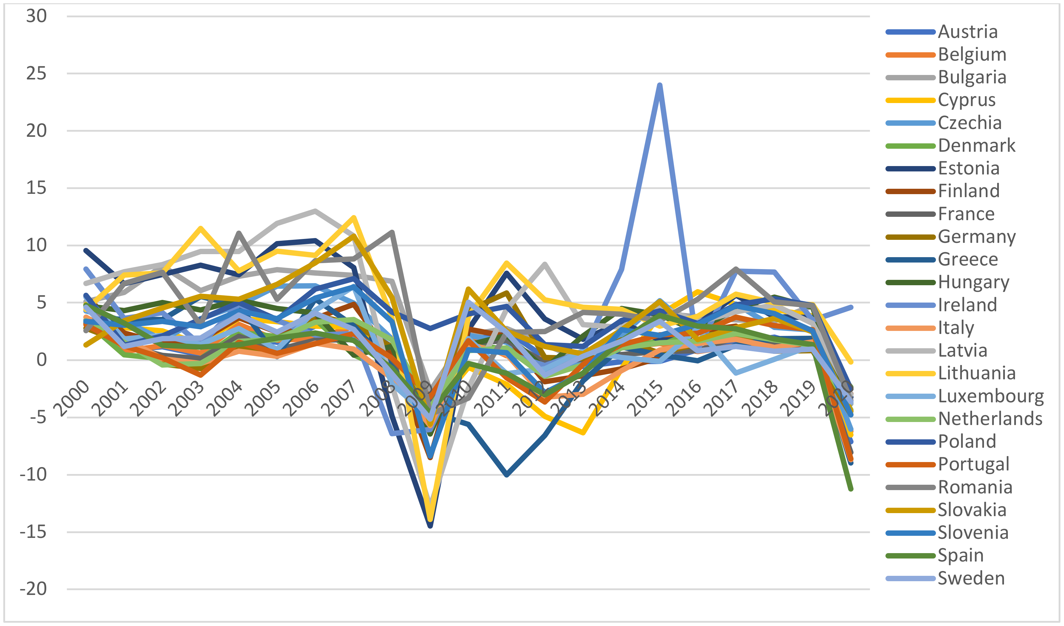
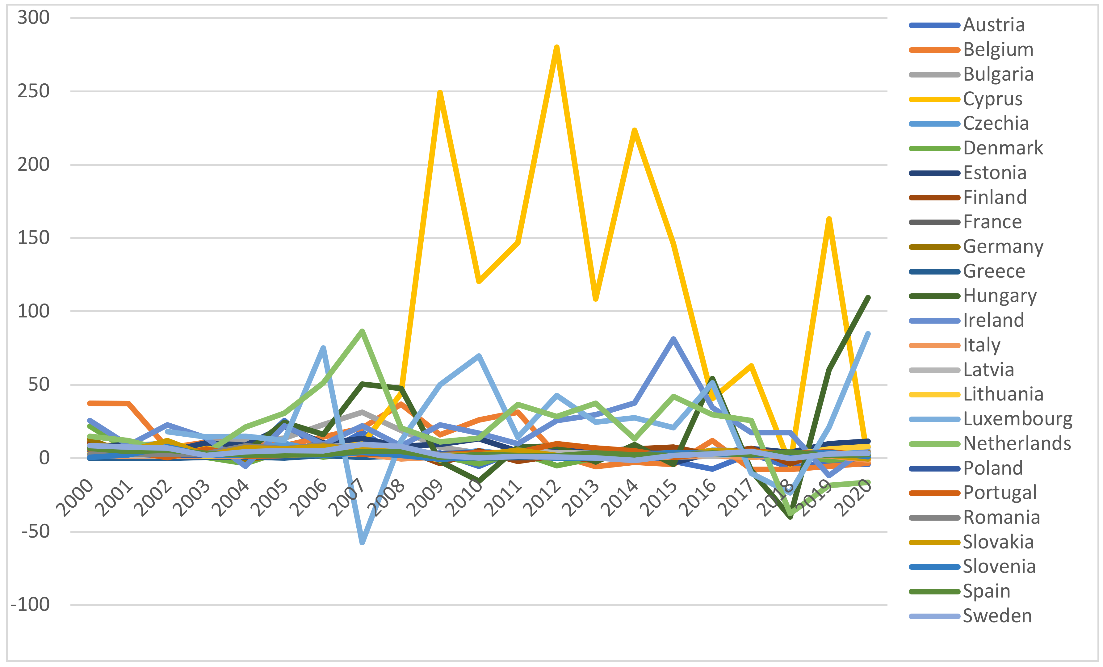
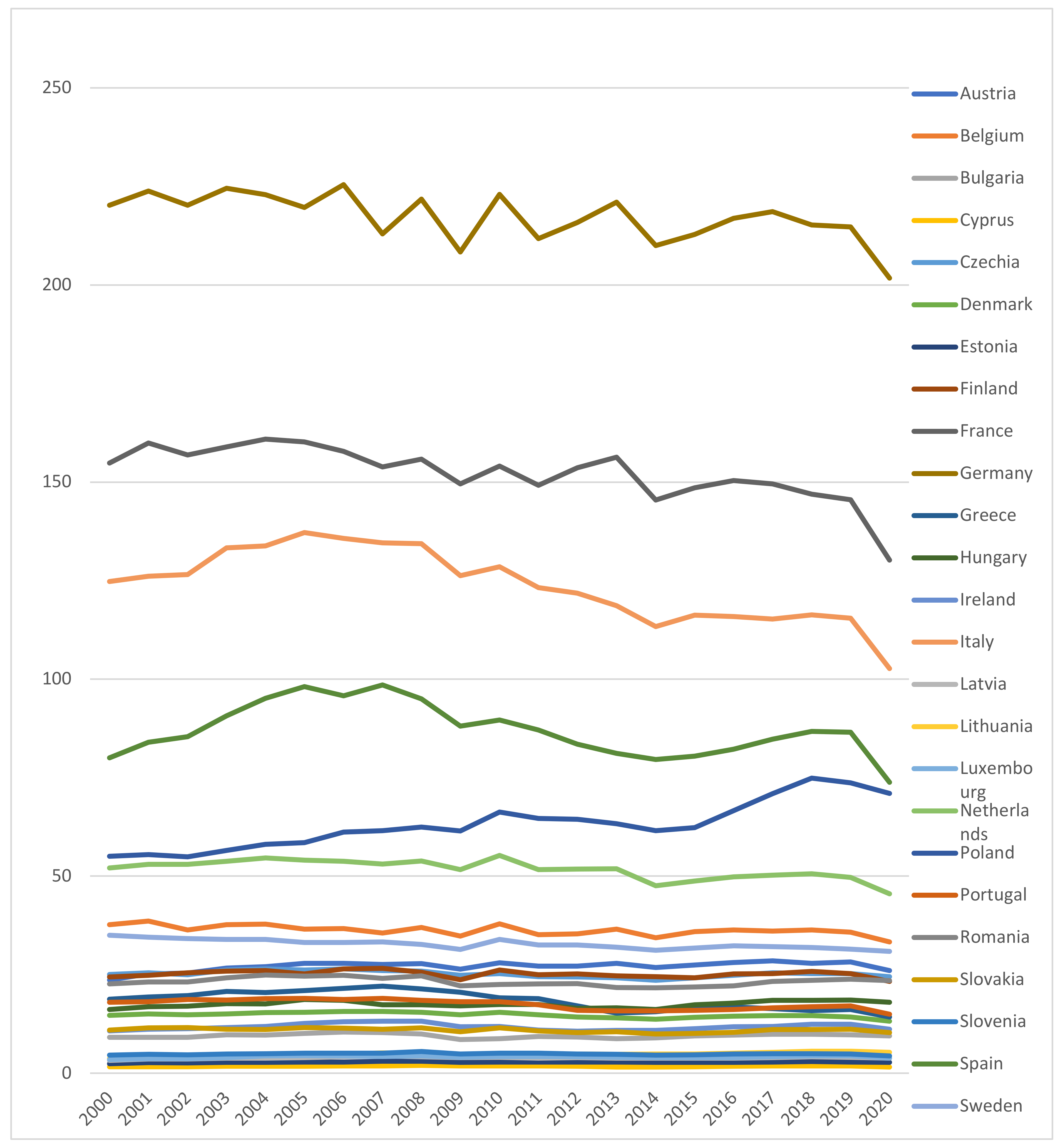
The evolution of the four variables for each country during the period of 2000–2020 is shown in Figure 2, Figure 3, Figure 4 and Figure 5. As can be seen in Figure 2, Luxembourg is one of the top European CO₂ per capita emitters. In 2020, Luxembourg ranked first among the CO₂ per capita emitters by applying emission reduction policies and experienced important changes from 19.7 metric tons per capita in 2000 to 15.3 in 2018 [60].

Figure 3 shows the evolution of the GDP annual growth rate during the analyzed period. As can be seen, in 2022, Ireland occupies the first place with a 10.9% increase in GDP, followed by Cyprus with 5.5% and Croatia with 5.2%.

In 2020–2021, the Netherlands and Luxemburg held together about half of the EU FDI stocks inward and outward. The highest peaks of the FDIs belong to Cyprus in 2009, 2012, 2014, and 2019, as seen in Figure 4. During 2015–2019, Cyprus’ innovation performance increased significantly and the FDI net inflows influenced positively the innovation climate, while its economy has been growing slowly. Cyprus’ GDP per capita is lower, but the business service sector development based on FDIs occupies an important place in the economy.

In the long-term, between 2005 and 2020, 23 EU member states reduced their energy consumption. As Figure 5 shows, Greece and Spain are on top. During the analyzed period, Germany, France, and Italy are the largest energy consumers in Europe.

We check the order of integration of the selected variables by four panel unit root tests belonging to the first generation: Levin, Lin and Chu, Im et al., and ADF-Fisher and PP-Fisher. Then, we apply second-generation panel unit root tests: CIPS by Pesaran [50].

Table 3. First-generation panel unit root tests.

At Level
Tests	Research Variables
	CO2	GDPG	FDI	ENCON
Unit root (Common Unit Root Process)
Levin, Lin, and Chu	4.5466 (1.0000)	−2.1038 (0.0177)	−3.8094(0.0001)	1.1232(0.8693)
Im, Pesaran, and Shin	6.0137 (1.0000)	−5.5563 (0.00)	−5.4198(0.00)	0.1690(0.5671)
ADF-Fisher Chi-square	21.7809 (0.99)	114.213 (0.00)	116.189 (0.00)	50.6494(0.4478
PP-Fisher Chi-square	20.1554 (0.99)	117.028 (0.00)	226.84(0.00)	79.8982(0.0046)
At first difference
Unit root (Common Unit Root Process)
Levin, Lin, and Chu	−2.9048 (0.0018)	−7.6484 (0.00)	−10.5248(0.00)	1.1016(0.8647)
Im, Pesaran, and Shin	−7.1101 (0.00)	−11.3079 (0.00)	−14.0774 (0.00)	−6.0897(0.00)
ADF-Fisher Chi-square	146.641 (0.00)	219.664 (0.00)	271.826(0.00)	125.965(0.00)
PP-Fisher Chi-square	293.100 (0.00)	491.121 (0.00)	1267.91(0.00)	665.969(0.00)

displays the first-generation panel unit root tests and

Table 4. Second-generation panel unit root tests (CIPS).

Variable	T-Statistics
	Level	First Difference
CO2	−1.92	−4.544 *
GDPG	−2.984 * 1	−4.285 *
FDI	−3.465 *	−5.381 *
ENCON	−2.155 ***	−4.345 *

¹ the symbols *, **, and *** refer to level of significance at 1%, 5%, and 10%.

displays the second-generation panel unit root tests. Table 3 reports the first-generation panel unit root tests statistics and the probabilities in parentheses.

FDIs and GDPG are stationary at the level, while ENCON and CO₂ are stationary at the first difference. The automatic selection by the Schwarz Info Criterion was used to determine the lag length.

From Table 3, we see that the variables have a mixed order of integration I(0) and I(1); none of the variables are I(2). Table 4 reports the cross-sectional dependence test results. The results of the CIPS unit root tests in Table 4 confirm that CO₂ is stationary at first difference, while GDPG, FDIs, and ENCON are stationary at the level. None of the variables are stationary at the second difference.

Therefore, it follows that the most adequate estimation procedure is panel ARDL, which provides more accurate results than a simple cointegration test.

We conduct the PMG, MG, and DFE techniques and we apply the long-run Hausman test to choose the best model. The null hypothesis of the Hausman test is that the PMG estimator is preferred while the alternative hypothesis is that the MG estimator is preferred. The p-value of the Hausman test is 0.48 greater than 0.05, thus we cannot reject the null hypothesis and we adopt the PMG estimator.

If we compare the PMG and DFE estimators, the null hypothesis of the Hausman test is that the PMG is preferred versus the alternative hypothesis that the DFE is preferred. The p-value of the Hausman test is 0.18 greater than 0.05; therefore, the PMG estimator is the most efficient one. It follows that the panel is heterogenous in the short-term and homogeneous in the long-term. The existence of a long-run relationship is that the pooled ECT should be negative, greater than −2, and statistically significant. In the three models, it satisfies these conditions. The PMG estimator is the most efficient estimator because, at the EU level, the long-term GDP growth should be targeted homogeneously, while in the short-term, each country should be treated independently and heterogeneously. In the short-term, each country should adopt its own strategy to increase its own economic growth, while in the long term, at the EU level and by EU policies, increasing economic growth should be a common target.

Table 5. PMG, MG, and DFE estimators.

Estimators	PMG		MG		DFE
Variables	Long-Run	Short-Run	Long-Run	Short-Run	Long-Run	Short-Run
Error Correction Term (ECT)	-	−0.6930	-	−0.7824	-	−0.6198
	-	(0.00)	-	(0.00)	-	(0.00)
ΔCO2	-	3.1765	-	2.5940	-	2.0825
	-	(0.00)	-	(0.00)	-	(0.00)
ΔENCON	-	3.7394	-	4.6741	-	0.2383
	-	(0.00)	-	(0.00)	-	(0.00)
ΔFDI	-	0.3076	-	0.1015	-	0.349
	-	(0.03)	-	(0.05)	-	(0.001)
CO2t−1	0.0084	-	1.78	-	0.0076	-
	(0.933)	-	(0.09)	-	(0.969)	-
ECONt−1	0.0416	-	−3.47	-	0.0670	-
	(0.257)	-	(0.08)	-	(0.451)	-
FDIt−1	0.0155	-	0.1015	-	−0.008	-
	(0.173)	-	(0.05)	-	(0.525)	-
Constant	-	0.2372	-	−6.39	-	−0.35
	-	(0.616)	-	(0.34)	-	(0.86)

reports the estimations of the long-run elasticities, the short-run coefficients, and the speed of adjustment to the long-run equilibrium. The ECT −0.69 is negative, greater than −2, and statistically significant at the 1% level. The speed of adjustment towards the long-run equilibrium is about 69% each year.

It implies that the system corrects its previous disequilibrium at an annual speed of 69%.

Regarding the short-term component (Table 5), the results proved that all coefficients are significant. There exists a positive and statistically significant correlation between the GDP growth rate and CO₂ emissions, energy consumption, and FDIs. A change of 1% in ENCON would lead to an increase of 0.0416% in GDPG. This result validates hypothesis H3. The same positive relationship is established by Esen and Bayrak [29]. It is well known that the energy sector is a driver of growth, its products being inputs for the production of goods and services. The energy sector is an important economic sector, creating jobs and impacting all the other sectors of the economy, sustaining economic activity.

A change in the CO₂ emissions of 1% leads to an increase of about 0.0084% in GDPG, confirming hypothesis H2. This positive correlation is validated by Azam et al. [12], implying that the EU countries use green technologies and follow the rules of environmental protection bodies. A change in FDIs of 1% leads to an increase of about 0.0155% in GDPG. This positive correlation is also confirmed by Sothan [34], Pegkas [35], Simionescu [36], Simionescu et al. [38], and Žarković et al. [37]. These results validate hypothesis H1.

The effects of FDIs are beneficial both for the host economy and the investor. Milutinović and Stanišić [61] underline the positive effects of FDIs on the economy, as seen by Kurtishi–Kastrati [62], such as capital, technology, and management transfer, creating employment in the host country, capital inflows, an increase in exports from the host country, and stimulate internal competition. The MG estimator results show that there is a long-run effect of the three regressors on GDPG at a significance level of 10%. The long-run results show that if there is a 1% increase in CO₂ and FDIs, the GDPG would increase by 1.78% and 0.10%, respectively, confirming hypotheses H1 and H2. A 1% increase in ENCON would lead to a decrease in GDPG by 3.47%, contradicting hypothesis H3. This correlation has been confirmed by the study of Sek (2017) for China, this being justified by a larger negative impact due to the indirect effect of CO₂ emissions. In the short-term, all three regressors have a positive significant effect on the output, confirming the three hypotheses. The ECT for the MG estimator is −0.78 and is statistically significant, which implies that the speed of adjustment is 78% annually. The DFE estimator results show that there does not exist a long-run effect of the three independent variables on economic growth if we take them individually because all the long-term coefficients are not statistically significant. In the short-term, all three regressors have a positive significant effect on the output, confirming the three hypotheses. In the short-run, a 1% increase in CO₂, ENCON, and FDIs lead to an increase of 2.08%, 0.23%, and 0.34%, respectively. The ECT for the DFE estimator is −0.61 and is statistically significant, which implies that the system corrects its previous disequilibrium at a speed of 61% annually.

In summary, the PMG and DFE estimators suggested that there exist only short-run causalities from CO₂ emissions, the energy consumption, and FDIs to GDP growth rate, confirming all three hypotheses, while the MG estimator proved the existence of both short-run and long-run causalities. The long-run causality confirmed H1 and H2 and contradicted H3. This study contributes to the literature by attempting to answer the research goal of whether there is a short-run and a long-run causality from CO₂ emissions, energy consumption, and the FDIs to GDP growth rate by checking hypotheses H1, H2, and H3. Our results can provide some insights for European and international environmental agencies. The choice of CO₂ as a single environmental indicator might limit the effects of environmental damage.

The industry is one of the main sources of pollution, which explains about half of the total emissions of GHG and air pollutants. This has important consequences on the environment, such as water and soil pollution and waste generation. Another source of pollution that comes from industrial activities is the burning of fossil fuels. The EU industrial policy plans to create a low-carbon industry, integrated into the flow of the circular economy, targeting reducing residual waste and air pollution.

This study has some limitations. One limitation is that the analysis is at an aggregated level, while an analysis of the economic sectors separately may provide a greater understanding of the relationship.

A future direction could be applying a structural break to determine the long-term relationship among the variables. Furthermore, this research should be continued with the quantile regression model or the quantile ARDL model. This paper can be continued with other studies in which several variables may be involved: urbanization, globalization, financial development, trade, or tourism. Another direction could be the use of other indicators than CO₂ emissions, such as municipal waste, energy use from transportation, other pollutants, etc.

5. Conclusions

In this paper, we applied the ARDL model with its three estimators: PMG, MG, and DFE to study the short-run and long-run impact of CO₂ emissions, energy consumption, and FDIs on economic growth, checking hypotheses H1, H2, and H3.

Applying the Hausman test, the most efficient estimator proved to be PMG. The ECT for all three estimators is negative and greater than −2, indicating that the system corrects its previous disequilibrium at an annual speed of 69%, 78%, and 61%, respectively. The MG estimator results proved a long-run and a short-run causality of all three regressors on economic growth, confirming H1 and H2 and contradicting H3.

In the short-term, all three estimators’ results confirm the three hypotheses.

Based on the findings of the paper, we can provide some recommendations for policymakers. To reduce environmental degradation and air pollution, governments should find alternate sources of renewable energy resources, reduce dependence on fossil fuels, and reduce geopolitical risks. Governments should stimulate businesses to promote renewable energy and install solar power and energy-based constructions. Streimikiene [63] emphasized the future role of renewable energy sources in households by installing electric heating and solar panels on the roofs of the buildings. Another direction in the literature on green energy is represented by energy poverty. Paper [64] compared the V4 countries (Hungary, Poland, Slovakia, and the Czech Republic) with the EU with respect to the energy poverty indicators. Some recommendations can be made, such as social support policies, improving energy efficiency, and using green energy. Paper [65] overviewed the research trends in the field of renewable energy and sustainability. The photovoltaic cells for solar panels become a central theme.

The public should become aware of these policies on environmental issues. Other environmental policies include increasing the infrastructure for energy efficiency, reducing unwanted waste, and finding new renewable energy sources to reduce pollutant emissions.