1. Introduction
This work is devoted to the assessment and analysis of the gross, technical and economic potentials of solar energy (see
Figure 1) for generating electricity through photovoltaic conversion.
Constant improvement of PV equipment is not the only factor affecting the increasing use of solar energy for electrification and the expanding implementation of PV systems. A great number of factors determining the development of photovoltaics are associated with the assessment of possible volumes of solar energy use in correlation with the technical and economic characteristics of PV equipment.
The values of solar energy potentials for different regions are necessary for the development of regional, state and interstate development programs, ecological programs, short-term and long-term forecasts, legislative instruments, and so forth [
1,
2].
Figure 1.
Three types of renewable generation potential (traditional ratio) [
3].
Figure 1.
Three types of renewable generation potential (traditional ratio) [
3].
The assessment of potentials is important both for implementing individual PV systems and for building and operating solar power plants [
4,
5,
6,
7,
8]. A correct assessment of potentials ensures maximally accurate forecasts at a macrolevel and optimal solutions on the placement, priority and financing of PV system implementation, interoperability between PV systems and other equipment, systems and facilities and choice of top-priority PV technologies [
9,
10].
Over recent years, much interesting research was pursued with respect to both worldwide assessment of solar energy potential and assessment of solar energy potential in individual regions [
3,
11,
12,
13,
14,
15,
16,
17,
18,
19,
20,
21,
22,
23]. That notwithstanding, an appropriate solar energy potentials assessment that is universal for various subsequent use options still remains a crucial task.
This is all the more so as solar energy is the only one from among the renewable energy sources for which a change in the traditional proportion between the gross, technical and economic potentials (see
Figure 1) is possible. Thanks to the development of integrated PV equipment (IPV), primarily building-integrated photovoltaics (BIPV) and building-applied photovoltaics (BAPV), the area for technical potential calculation in populated regions may be considerably greater than the Earth’s surface area used for calculation of the gross potential. That is, taking into account BIPV and BAPV, the technical potential of solar energy may be greater than the gross potential (see
Figure 2).
The analysis showed that even the most evident indicator, i.e., the unit gross potential (that is equal to solar irradiation), is evaluated in various ways for one and the same territory in different sources.
For the purposes of building new PV facilities, a wide variety of estimates are proposed: from very crude and rough (as, for example, in [
24]) to more or less accurate [
25,
26,
27,
28]. In [
24] the technical potential of solar energy in a region, if planar modules are used, is estimated as the solar energy arrival at 1/5 of the region’s area multiplied by the modules’ efficiency factor. In [
25] the gross, technical and economic potentials of solar energy are determined for 26 different regions of the Earth subject to various possible restrictions on the surface.
In [
26] the values of potentials are computed using the geographic information system for the Krasnodar Region. In [
27] the solar energy potentials in the Greater Mekong area are considered for the purpose of forecasting the cost of energy received from any kind of renewable energy sources (including solar energy). In [
28] the NASA data on the solar energy arrival and temperature are used. RETScreen software was used to calculate the economic potential for 22 different locations in Libya. The best location was found for a network solar power plant. In [
29] it is proposed to use roofs for placing solar modules on them. Numerical simulation was used to compute the gross and technical potentials for 11 regions in the world. It is noted that the use of roofs for generating electric and heat energy may result in a considerable saving of heat and electric energy.
Top-down methodology [
30,
31] takes into account mineral reserves, land competence and other limits which are not considered by other authors. Such an approach is indeed important for global estimates for a long period of time. In case of relatively short-term estimates, the consideration, for instance, of mineral reserves makes no sense except if their development and use is fully prepared for launch. The research of the same authors [
32] is one of those we based our own on when elaborating out approach. We completely agree that “many of the estimations found in the literature are hardly compatible with the rest of human activities.” However, the meaningful constraints on the use of solar energy for photovoltaic energetics, which in their opinion exist, do not relate to the solar energy.
2. General
The smart analysis includes the basic program working under the condition of connection to databases and to the programs of determining required initial data or, as a limited option, under the condition of full or partial initial data input by the user.
Thus, in the optimal variant, a smart network is formed, which for the purposes of obtaining the values of potentials uses the most up-to-date values of initial data and other required information that is received, processed and calculated in parallel with the calculation of potentials.
A program extension is envisaged which enables a more detailed analysis, both for a territory of a lesser area and for a greater amount of initial data or their variants that is taken into account, and also a comparative outcome analysis using the specified assessment criteria. In this case, the matrices of potentials values for various options and comparison results are released at the output.
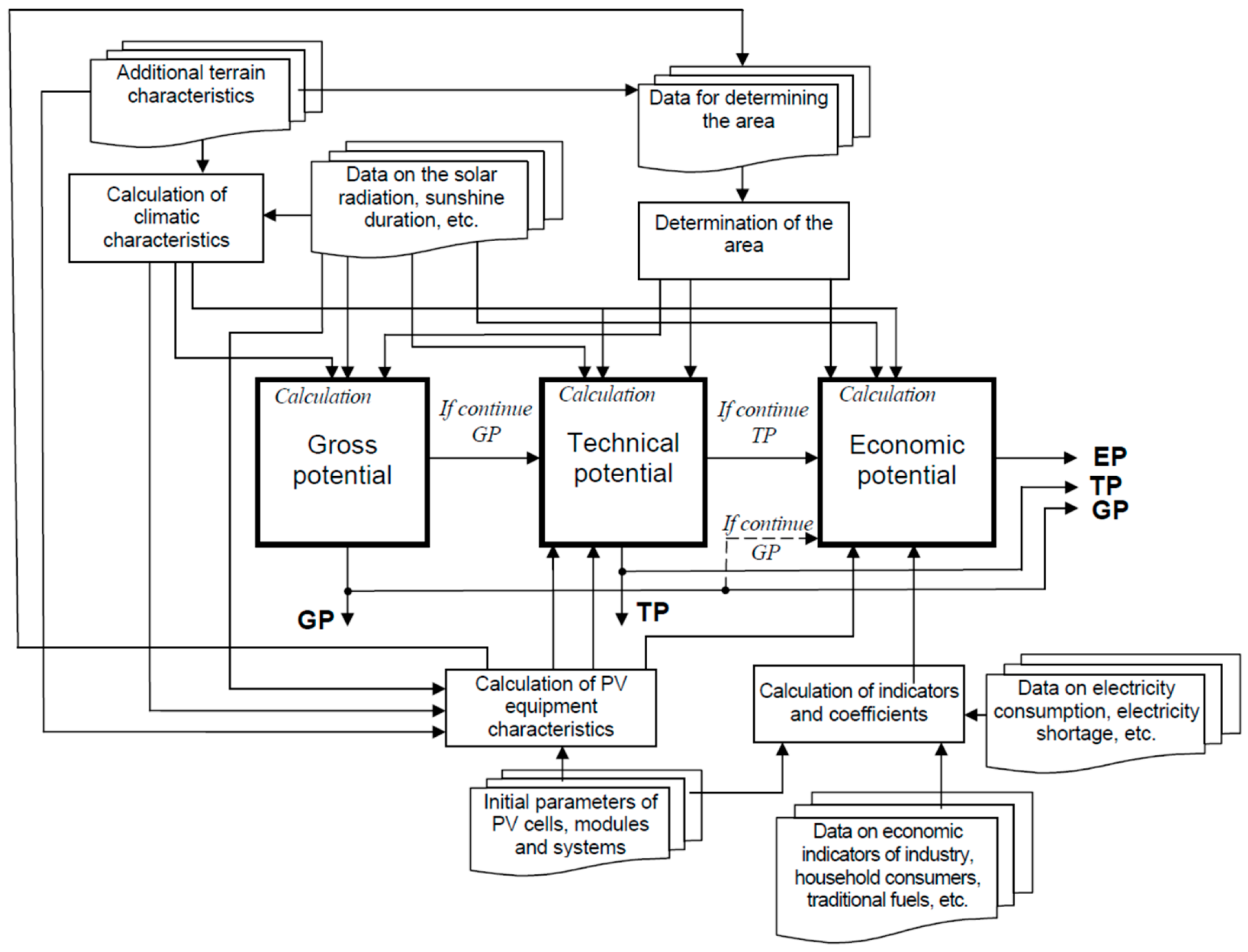
This article provides the description of the basic analysis algorithm (“central steps”).
Figure 3 shows the general diagram of the calculation logic. If the gross (GP), technical (TP) and economic (EP) potentials are determined within the same task, the calculation is performed sequentially starting from GP. While calculating the subsequent potential, the calculation results for the previous potentials are used, for example the calculated values of solar irradiation on the active surface of PV modules, their operating temperatures, and so on.
A region is the total of K areas, or zones, in which the density of incoming solar energy and the Earth’s albedo, as well as geographical, climatic and weather conditions are homogenous throughout the total area of the zone. Such zones have the linear dimensions of up to ≈200 km. The number of zones in the region, their locations and areas are set out in a separate table.
The results are released as the values of potentials (kW∙h/yr), where the calculated area is determined, and/or, if more universally, as the specific values of potentials (kW∙h/m2∙yr).
The technical and economic potentials are determined considering BIPV.
The minimum scope of calculations is as follows: month, zone, the most popular type of PV modules, overall economic indicators of industrial and domestic consumers.
The calculations are performed for two ultimate options of solar irradiation on the active surfaces of PV modules based on the adopted variants of their orientation and installation: a permanent installation at the optimal tilt angle to the horizon and a continuous tracking of the sun when using solar radiation concentrators. The program assumption is that the modules operate with free air movement around them, i.e., they are installed in an open rack.
The extensions allow calculations to take into account additional factors influencing the module irradiance and temperature by connecting to other programs or values/coefficients entered by the user, e.g., to consider air pollution in the region and the pertinent change in the radiation spectrum.
3. Determining the Gross Potential of Solar Energy in a Region
3.1. General Formula for Calculating the Potential
The gross (theoretical) potential of solar energy in a region for photovoltaic energetics, hereinafter the “GP” (kW∙h/yr), is the long-time average total energy of solar radiation arriving at the region’s area in one year.
The gross potential of the region is the sum of gross potentials of the zones forming it:
Depending on the volume and nature of the initial data used, the calculation of the gross potential of solar energy in a zone is performed using the following three options.
3.2. Determining the Gross Potential of Solar Energy in a Zone Subject to the Volume and Nature of the Initial Data Used
3.2.1. There Is a Weather Station or Satellite-Based Measurement Data Are Used in the Zone
If meteorological data on the long-term average of incoming solar energy for each month of the year are available, the total solar irradiation is calculated according to the following formulas:
where
Hj is the long-time average annual total solar irradiation in the
j zone, kW∙h/(m
2∙yr);
H is the long-time average annual solar irradiation in region, kW∙h/(m
2∙yr);
Hi is the long-time average annual solar irradiation on horizontal surfaces in the
i month of the year, kW∙h/(m
2∙mo);
Hd i is the long-time average annual direct solar irradiation on horizontal surfaces in the
i month of the year, kW∙h/(m
2∙mo); and
Hdef i is the long-time average annual diffuse solar irradiation on horizontal surfaces in the
i month of the year, kW∙h/(m
2∙mo).
The gross potential of the j zone is determined as follows:
and for the region, Equation (1) has a similar form:
In Equations (5) and (6), Sj and S are total areas of the j zone and region, respectively (m2).
The calculated values of Hi, Hdi and Hdefi, Hj, GPj and H (if necessary) are used to create a table. In addition, the meteorological data (if any) on the root-mean-square dispersion of solar irradiation (as absolute values or percentage) are inserted into the table.
Similarly, a calculation is performed using the satellite-based data, for example, the NASA database. However, when choosing such a calculation option, it should be taken into account that these data do not involve to the full extent the peculiarities of solar radiation arriving on the active surface of PV modules.
3.2.2. There Is No Weather Station in the Zone
Where there are no meteorological data on solar irradiation but the neighboring weather station data are known and may be used for determining the average values of sunshine duration for each month of the year, Hi is determined in the following manner.
To calculate the solar irradiation, an indirect method is employed through the use of the radiation data obtained at the neighboring weather stations and in the adjacent territories and with the application of the Angstrom formula [
33] improved by [
34]. The average monthly total solar irradiation is determined according to the following formulas:
where for the
i month of the year:
H0i is the long-time average annual solar irradiation on horizontal surfaces under clear sky, kW∙h/(m
2∙mo);
ai and
bi are the empirical coefficients (
ai +
bi = 1) calculated for
k trapeziums by which the analyzed territory is broken down for each month (see, for example, [
24]);
is the average intensity of solar radiation on the active surface of PV modules for atmospheric mass
M (W/m
2);
θi is the angle between the sun vector and the zenith vector (angle of incidence on horizontal surfaces);
is the empirical duration of sunshine for the locality in question during the month, h/mo; and
t0i is the astronomically possible duration of sunshine for the given locality during the month, h/mo.
The factors of Equation (8) for the
i month are determined using the following formulas:
where
G0 = 1360 W/m
2 is the solar constant;
G1 is the direct solar irradiance corresponding to terrestrial solar radiation in the southerly latitudes at sea level and on a clear day—these are approximately the conditions of atmospheric mass
M = 1,
G1 = 1000 W/m
2;
δ is the mean solar declination that is determined by the Cooper formula [
35] (see
Table 1), rad;
ωs-si is the sunrise–sunset angle in the
i month, rad; and
ni is the number of days in the
i month.
The angle
ωs-si is determined by the following formula:
The Calculation Procedure
The parameter values of φ, δi, ai, bi, ni and tsi for each month of the year in this zone are the initial data for calculations.
The parameter values of ωs-si, t0i, , Mi, , H0i and Hi are consequently calculated for each month of the year in this zone using Equations (7)–(13).
Using Equations (2), (4) and (5), the calculation of Hj, H and GPj is completed and the table of values of Hi, Hj, H and GPj is formed.
3.2.3. The Data on Solar Irradiation on Inclined Surfaces Are Available
If there are only data on long-time average annual solar irradiation in each month on a surface inclined at the angle
β to the horizontal and oriented to the south,
Hti (W∙h/(m
2∙mo)), the monthly solar irradiation
Hi is calculated using the following formulas:
or
where
ωmax is the astronomically possible hour angle of maximum insolation of the inclined surface, rad; and for the
i month of the year:
βopt i is the optimal angle of inclination of the PV module active surface to the horizontal;
ξi is the angle between the sun vector and the normal line to the inclined surface (angle of incidence on the inclined surface) oriented to the south;
εi =
Hdi/
Hi is the share of diffuse radiation in the total solar radiation; and
ρi is the ground surface albedo.
The average value
determines the average flow of solar radiation falling on the inclined surface in the day’s interval of hour angles of the inclined surface insolation Δ
ω:
where
ω = π
t/12 is the hour angle of solar motion that is equal to 0 at solar noon; each hour of time
t corresponds to 15° of longitude, and the values of an hour angle before noon are deemed positive, while those after noon are deemed negative.
For the ‘winter’ half of the year (
δ ≤ 0)
ωmax =
ωs-s. For the ‘summer’ half of the year (
δ ≥ 0)
ωmax =
ωS, where
ωS is the hour angle of the sun meeting the condition of cos
ξ = 0, and
For calculating the optimal value of the inclination angle,
βopt is used, which is determined as follows:
There are two options, depending on the chosen accuracy of calculations: βopt i = βopt = constant for all months of the year and βopt i = variable.
The Calculation Procedure
The parameter values of φ, βopt i, δi, εi, ρi and Hti for each month of the year in this zone are the initial data for calculations.
The parameter values of ωs-si, ωS, , and Hi are consequently calculated for each month of the year in this zone using Equations (11), (13)–(16) and (18).
Using Equations (2), (4) and (5) the calculation of Hj, H and GPj is performed and the table of values of Hi, Hj, H and GPj is formed.
Upon the potential of each zone being calculated, the gross potential of the region GP is calculated using Equation (1) as the sum of the gross potentials of the zones.
4. Determining the Technical Potential of Solar Energy in a Region
4.1. General Formulas for Calculating the Potential
The technical potential of solar energy in a region for photovoltaic energetics, hereinafter the “TP” (kW∙h/yr), is the long-time average electrical energy which may be generated in the region through photovoltaic conversion of solar radiation in one year with the current state of the art in science and technology and subject to environmental compliance.
The technical potential of solar energy is the sum of the technical potentials of thermal energy and electrical energy obtained through conversion of solar radiation.
The technical potential of the region is the sum of the technical potentials of the zones forming a part of it:
The technical potential of a zone is determined as follows:
where the technical potential of the
i month in the
j zone, subject to the chosen position of the surface at which solar radiation arrives, is equal to:
or
where
STPj is the portion of the
j zone area which economically and environmentally is reckoned to be expedient for installing PV systems (without regard to BIPV, AgroPV, etc.), m
2; it is equal to such portion of the total area of the zone
Sj as is left after deducting the territories in which the placement of PV systems/PV modules is prohibited:
Ti is the average monthly operating temperature of a PV cell, K;
T1 is the operating temperature of a PV cell in the agreed standard lighting conditions (
GM1 = 1000 W/m
2),
T1 = 25 °C = 298.15 K;
η1 is the efficiency factor in the agreed standard lighting conditions;
χ is the temperature gradient which depends mainly on the PV cell type and design.
The calculation takes into account that the efficiency of PV cells, PV modules and, accordingly, PV systems is a composite function of lighting intensity and spectral structure, and the operating temperature of elements which may change in a random way. The calculation logic is based on the fact that as the operating temperature
T1 rises, the efficiency factor decreases (see, for instance [
36,
37]). This is chiefly originated by the linear drop in the no-load voltage,
Vo.c, because of the sharp exponential growth in the reverse saturation current,
J0, and the relevant decrease in the volt-ampere characteristic filling factor,
FF [
38]. Contemporaneously, the photocurrent,
Jf, increases, but very weakly, so that the full temperature gradient of the efficiency factor turns out to be negative and the explicit temperature dependence of the efficiency factor for lightning, AM 1, is represented as follows:
For the purpose of uniform valuation, the values of the parameters in the agreed standard lighting conditions, AM 1 (GM1 = 1000 W/m2), are used at an operational temperature of T1 = 25 °C = 298.15 K.
The average monthly temperature of a PV cell [K] is equal to:
where
α is the integrated coefficient of solar radiation absorption by the photovoltaic elements of PV cells;
λ is the coefficient of heat transmission from the surface of PV modules or the radiator of concentrator photovoltaic (CPV) modules (W/(m
2∙K);
is the average monthly environmental temperature during daylight (during the operation of PV systems), K;
tPVi is the average duration of PV systems operation in the
i month, h;
tPVi ≤
tsi and is determined based on the value of
tsi and the number of clear, overcast and partly overcast days in the zone. If there are no data on the number of clear, overcast and partly overcast days in the zone, it is taken that
tPVi =
tsi.
Should the potential be determined for any specific types of PV modules which, for example, underwent tests under the IEC 61853-2 [
39], i.e., the empirical ratios of module operating temperature to wind speed are known for them, then the average monthly temperature of a PV module is calculated as follows:
where
u0 is the coefficient reflecting the influence of irradiance on the PV module temperature;
u1 is the coefficient reflecting the influence of wind speed on the PV module temperature;
is the average value of wind speed in the
i month.
With this, it is taken that the temperature difference (Ti − Tamb) actually does not depend on the environmental temperature and generally is directly proportional to irradiance at 400 W/m2 or more. In general, both coefficients depend on the method of installation of a PV module.
4.2. Procedure for Calculation
Unless otherwise specified, the initial data for calculations are the values of the parameters characterizing the current technical level of the most common flat silicon PV modules:
α, η1,
χ and <
λ>, as well as the data for calculating the solar irradiation in respect of each zone as set out in
Section 3.2, and
, data on the number of clear, overcast and partly overcast days in the zone.
The calculations are performed for each zone as follows.
The total solar irradiation on the active surface of PV modules,
Hi or
Hti, is calculated as described in
Section 3.2.3. The average monthly operating temperature in the
j zone is calculated.
The technical potential of the i-month, TPi, is calculated.
The technical potential, TPj, of the j zone is determined by summing up all the months, and the table of values of Ti, Hi or Hti, TPi and TPj, is formed.
Upon the technical potential of each zone being calculated, the technical potential of the region TP is calculated by Equation (20) as the sum of the technical potentials of the zones.
The algorithm allows several options for the initial data values to be proposed, for instance, for different technologies of PV module manufacture for all zones or different values for different zones, and then comparison and selection or valuation to be carried out, as well as taking into consideration the particularities of BIPV, BAPV and AgriPV.
5. Determining the Economic Potential of solar Energy in a Region
5.1. General Formulas for Calculating the Potential
The economic potential of solar energy in a region for photovoltaic energetics, hereinafter the “EP” (kW∙h/yr), is the amount of annual generation of electrical energy in the region through the use of photovoltaic conversion of solar radiation, the generation of which energy is economically justified for the region at the existing level of energy and fuel production, transportation and consumption prices and subject to environmental compliance.
The economic potential of the region is the sum of the economic potentials of the zones forming a part of it:
The economic potential of the
j zone is determined as the sum of the potentials of each month of the year:
Therefore, the economic potential of the
i month for each zone is determined as follows:
where
Wi is the amount of electric energy generated by PV systems per unit area of the active surface of PV modules or aperture of CPV modules (unit generation) in the
i-month, kW∙h/(m
2∙mo) [
40,
41];
SEPj is the economically expedient area of PV systems placement in the
j zone, m
2.
The generation of the PV systems installed in the territory is calculated according to the following formulas:
The
j zone in the
i month
annual generation of the
j zone
in the
n year
annual generation of the region
where
HPVi is the solar irradiation on the active surface unit of PV modules or aperture of CPV modules in the
i month and
kn is the maximum capacity degradation of PV or CPV modules in the
n year,
n = 1, 2, …,
ts.
There are two ultimate options for determining the economic potential.
In the first option, PV modules are considered to be permanently oriented at the optimal angle of inclination to the horizontal
βopt. With this,
HPVi = Hti is determined by Equations (14) or (15) provided that the average value
is determined as follows:
In the second option, a PV system is composed of CPV modules [
42] with continuous tracking of the sun and:
where
Hni is the solar irradiation on a normally oriented surface;
K is the solar radiation concentration ratio.
5.2. Determining the Economic Parameters of PV System Use
The annual economic effect of using PV systems in the region
E (€ or
$, etc.) is determined as the sum of economic effects of using PV systems in each zone:
The annual economic effect for each zone is as follows:
where
ts is the service lifetime of PV systems, year;
ct.s.e j is the unit cost of energy production using traditional sources subject to the regional fuel cost factor and regional ecological factor, EUR/(kW∙h) or USD/(kW∙h);
closs j is the unit cost of losses from energy shortage or unit cost of the valuables produced by industry in the
j zone, EUR/(kW∙h) or USD/(kW∙h);
Dj is the annual electrical energy deficit and/or additional demand of industrial production for electric energy in the
j zone
, kW∙h/yr;
Wcrit j is the critical value of annual generation by PV systems determining the field of economic expediency of their use in the
j zone, kWt∙h/(m
2∙yr).
where
rt.s.ej is the regional ecological factor of traditional energy sources;
rcj is the regional factor of traditional source energy cost;
ct.s is the unit cost of energy production using conventional energy sources, EUR/(kW∙h) or USD/(kW∙h).
If monthly data are available, then:
The critical value of specific generation by PV systems
Wcritj is determined as follows:
where
rej is the territorial ecological factor of using PV systems;
cPVj is the unit final cost of PV systems (before the date of putting them into operation), EUR/m
2 or USD/m
2 and
γ is the standard cost of operation, 1/year.
The payback time for PV systems
tpb (year) is calculated according to the following formula:
5.3. Economic Potential Assessment with Different Relationships of Service Lifetime and Payback Time
In accordance with the definition, the economic potential of solar energy in a region for photovoltaic energetics is the energy which may be generated during the year by the PV systems installed in the territory, provided that their economic effect is positive or equal to zero:
The feasibility analysis of this condition provides for two options.
- (1)
Where the service lifetime of PV systems is longer than, or equal to, their payback time:
i.e., if the specific generation by PV systems is greater than, or equal to, its critical value:
then, by virtue of a usual condition:
The economic potential of using PV systems is positive with any number of installed PV systems, no matter how much area fit for this they occupy. This means that in this case it is expedient to use the greatest possible number of PV systems, i.e., the active surfaces of PV modules will occupy the greatest possible area and the economic potential of solar energy in the region for photovoltaic energetics turns out to coincide with its technical potential:
- (2)
Where the service lifetime of PV systems is shorter than their payback time:
i.e., if the specific generation by PV systems is greater than, or equal to, its critical value:
then the fulfillment of the condition of Equation (41) is in line with the following limitation of the PV system full capacity:
and concurrently
Provided that the service lifetime is close to the payback time or, more precisely, if:
then the economic potential, as in case 1, is equal to the technical potential, Equation (45).
If the condition of Equation (49) is fulfilled, i.e., when:
the economic potential of solar energy is equal to:
And finally, in the realm of:
the economic potential is equal to zero:
where the condition of Equation (53) is fulfilled, the cost of the energy produced by PV systems is so high that the products of industry manufactured with their use do not cover, in terms of cost, the electric power costs, i.e., the use of this power plant is inexpedient.
Even for different zones of the region we can envisage different scenarios of economic potential assessment of the same type of PV systems, which is subject to climate and energy consumption features. Accordingly, the values of zone economic potentials are determined by Equations (45), (52) or (54).
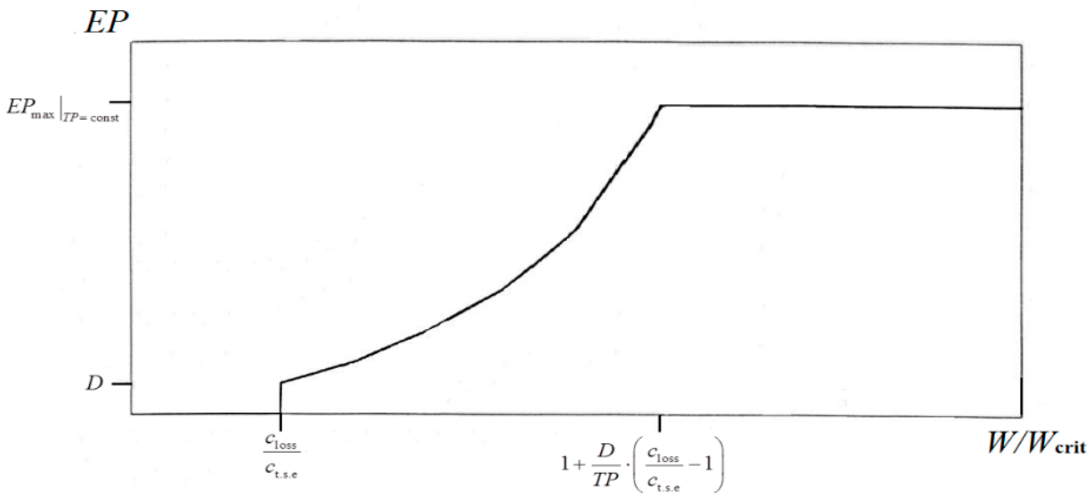
The economic potential of solar energy in the region,
EP, is increasingly dependent on the annual amount of energy obtained from the active surface unit of PV modules,
W, which is determined by three parameters: critical value of energy generation,
Wcrit, demand of industry and domestic consumers in the region for electric energy,
D/TP, and price,
closs/
ct.s.e. The typical correlation is shown in
Figure 4.
For the purpose of assessment, the notions have been introduced of surplus of economic potential of solar electric energy in the region and zone, Δ
EPj and Δ
EP, constituting the difference between the economic potential and the total demand for electric energy in the region/zone:
and
where
Q is the region’s total demand for electrical energy, kW∙h/yr, which is the sum of demands for electrical energy on the part of production,
Qp, and domestic consumers,
Qd:
The zone’s total demand for electric power, Qj, is determined in a similar way.
If ΔEP > 0 or ΔEPj > 0, a region or zone, respectively, is an economically justified potential donor of electrical energy.
5.4. Procedure for Calculation
Option 1: PV systems are composed of flat PV modules permanently oriented at an angle of inclination to the horizontal that is βopt.
The initial data for calculations are the initial data set out in
Section 3: service lifetime of PV systems,
ts, maximum capacity degradation,
kn, for a year of service, as well as the values for each zone of
cPV, factors
rt.s.e,
rc,
re and
ct.s.e,
closs,
D (or
closs.i,
Di in each month of the year for each zone), values of
Qp,
Qd and
Qpj,
Qdj for the region and each zone, respectively.
The calculations are performed for each zone in the following manner.
The solar irradiation on the active surface of PV modules placed at the angle of inclination to the horizontal,
βopt and
Hti, and the average monthly operating temperature in the zone
j, are calculated as described in
Section 2 subject to Equation (33). Alternatively, the values which were obtained when calculating the technical potential are used if the calculations of both potentials are performed together.
Consecutive calculations are performed for the generation by PV systems, Wi, for each month of the year (using Equation (29)), annual generation in the j zone, Wj, (using Equation (30)), and generation in the region, W (using Equation (32)) and Wcrit (using Equation (39)).
The fulfillment of the conditions for Equations (43), (50), (51), (53) is analyzed and the region of definition of economic potential is determined. The potential value, EPj, is calculated.
Qj and the surplus potential ΔEPj are calculated.
Option 2: PV systems are composed of CPV modules which are oriented to, and continuously keep track of, the sun.
The initial values of the parameters are the same as for option 1, with the exception of the PV system cost, cPV, which, in accordance with the practical data for option 2, is taken to be equal to C/3 with K = 13, and the temperature coefficient of the efficiency factor, which is theoretically and practically less and is taken to be equal to χ = 0.003 K−1.
With regard to each zone, the values of Hni are calculated by Equation (34) for i = 1, 2, …, 12. Then, calculations are performed similarly to option 1, and EPj and ΔEPj are determined.
After comparing the values of economic potential under the two calculation options, the greater value is chosen which is taken as the economic potential of solar energy in the zone EPj.
Upon the economic potential of each zone being determined, the economic potential of the region is calculated by Equation (26) as the sum of economic potentials of the zones.
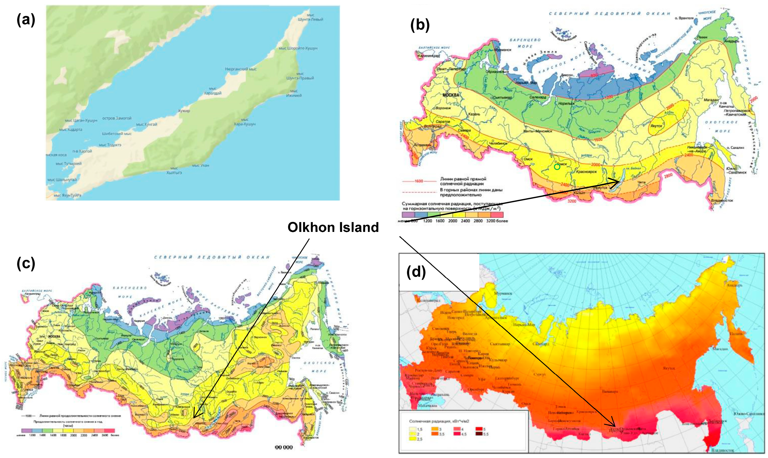
6. Example of Solar Energy Potential Assessment for Photovoltaic Conversion in the Olkhon District of the Irkutsk Region (52° N and 105° E)
6.1. Climatic Conditions
The Island of Olkhon is situated in Lake Baikal and its geographical coordinates are 52° north latitude and 105° east longitude (see
Figure 5). The island area is
S = 730 km
2.
There are weather stations in the settlements of Khuzhir and Uzur, and there was a weather station in Cape Tashkai before 1964. The entire territory of the island is considered a single zone, and the potentials of the Island of Olkhon are calculated as the potentials of a zone.
Some characteristics of solar irradiation on horizontal surfaces and the reflecting power of the earth’s surface are set forth in
Table 2 and
Table 3. All of the calculations are performed in terms of local time.
The air temperature during daylight hours for different months of the year, to the exclusion of the ‘darkest’ months, November, December and January, is shown in
Table 4.
For November, December and January there are average temperature data during daylight hours based on the average daily temperature in the pertinent month: = −5 °C; = −11 °C; = −17 °C.
The total solar radiation on horizontal surfaces was calculated using the data from
Table 4 (by the number of sunny days) and the data from
Table 3. For example, for March the calculation was as follows:
The share of diffused radiation, ε, for each month specified in
Table 4 is determined as the ratio of diffuse irradiation to total irradiation for the relevant month and calculated using the data from
Table 3 and
Table 4. For instance, for March this is:
Hence, during the time of year that is the most efficient for using solar energy the average share of diffuse radiation is about 0.3 of the total irradiance. It should be noted that in the autumn and winter period (October to February), the share of diffuse radiation grows sharply, so that the average yearly share of diffuse radiation in the total solar radiation is about 0.4.
For comparison and supplementation of
Table 4,
Table 5 provides data on monthly and annual solar radiation on surfaces inclined at 45° to the horizontal in the weather station nearest to the village of Khuzhir, situated in Irkutsk.
6.2. Gross Potential of Solar Energy
In accordance with Equations (1), (2) and (5), for determining the gross potential, it is necessary to obtain the data on monthly solar irradiation on horizontal surfaces, Hi (i = 1, 2, …, 12).
The values of
Hi, calculated and set out in
Table 4, relate to the seven sunniest months, with
i = 3–9. In order to calculate the solar irradiation in other months (
i = 1, 2, 10, 11, 12), it is expedient to use the data on monthly irradiation on inclined surfaces, presented in
Table 5, in accordance with the methodology described in
Section 3.2.3.
Table 6 contains the average monthly parameters for these months, calculated using coefficients from Equations (15)–(18) for the Khuzhir latitude,
φ = 52°.
The results of calculating the mean angle of inclination of direct solar radiation to the normal line, <cos
θi>, and monthly direct solar irradiation on normally oriented surfaces,
Hd.ni, during a 10 h period (from 07 a.m. to 05 p.m.) for each month of the year are represented in
Table 7. The values of
Hd.ni were calculated using Equation (34) using the following formula:
Considering that the territory under analysis was not divided into zones, the solar irradiation on horizontal surfaces unit per annum is determined using Equation (2) as follows:
and the gross potential of Olkhon is:
6.3. Technical Potential of Solar Energy
The initial data are the initial data in
Section 6.2, as well as the parameter values characterizing the current state of the art for the most commonly encountered flat silicon PV modules:
The values of the average monthly operating temperature,
Ti, calculated by Equation (24) using the values of
Tambi (
Table 2),
Hi (
Table 4 and
Table 6) and
tsi (
Table 4) are set out in
Table 8. The average PV system operation time,
tPVi, from March to September was determined using the values of
tsi and the number of clear, partly overcast and overcast days in the month (
Table 4). For autumn and winter months (
i = 1, 2, 10, 11, 12), which make a small contribution to the potential, the following approximate relationship was used:
tPVi =
tsi = 0.9
t0i.
Table 8 represents the values of the monthly technical potentials per surface unit of the Island of Olkhon where PV systems may be installed. These potentials were calculated using Equation (22) by the following formula:
The potential
TP under Equations (20) and (21) is determined by summing up all of the months, taking into account that the territory of the island is deemed one zone and, therefore,
with
j = 1:
6.4. Economic Potential of Solar Energy
6.4.1. Initial Data
The initial data are the initial data in
Section 6.3 or/and calculation results in
Section 6.3, as well as the characteristics of PV systems: unit final cost subject to the ecological factor,
cPV.e (
cPV.e =
cPV ∙
re = 510 USD/m
2 = 30,600 RUB/m
2).
Furthermore, the following apply to the levels of power supply to people and industry in the Island of Olkhon:
Unit cost of traditional fuel subject to the regional and ecological factors for 2022 in renominated prices ct.s.e = 15.25 RUB/kW∙h;
Demand of industry for electric energy D = 818 MW∙h/yr;
Unit cost of losses from electric power shortage (unit cost of industrial products) (assessment by the order of values) closs = 100 RUB/kW∙h;
Population N = 1744 people;
Domestic demand of population for electric energy Qd = 1159.18 MW∙h/yr.
6.4.2. Parameters of PV Systems Equipped with Traditional Planar Silicon PV Modules
The solar irradiation on the active surface unit of PV modules,
HPVi, is equal to the values of solar irradiation on surfaces tilted at the angle
βopt (Equation (19)) to the horizontal,
Hti. Using the values of
Hti and ambient temperature,
Ti, determined as specified in
Section 6.2 and
Section 6.3, the generation by PV systems installed on the island area unit,
Wi, is calculated by Equation (29) for each month of the year and for a 10-h interval (from 07 a.m. to 05 p.m.). The results are set out in
Table 9.
The annual generation in the year of systems installation (
kn = 1),
W1, is determined by summing up
Wi for all the months of the year using Equations (30) or (31):
6.4.3. Parameters of PV Systems Equipped with CPV Modules with Continuous Tracking of the Sun
The initial parameter values are the same as in
Section 6.4.2, except for the PV systems cost, which in accordance with the practical data is taken to be equal to
cPVe/3 with
K = 13 and the temperature coefficient of efficiency factor, which is theoretically and practically lower than expected and considered to be equal to
χ = 0.003 K
−1.
The values of
HPVi are calculated by Equation (34) for
i = 1, 2, …, 12 using the values of monthly solar irradiation on normally oriented surfaces,
Hd.ni, and values of <cos
θi> (see the calculation in
Table 7). The other calculations are performed similarly to those for PV systems fitted with planar silicon PV modules. The results are set out in
Table 10.
The annual generation in the first year of systems operation is:
Hence, the unit energy generation by CPV modules with continuous tracking of the sun turned out to be approximately equal to the unit energy generation by ordinary planar PV modules, so the conclusion on expediency of using modules of any design depends on economic indicators.
6.5. Economic Potential Subject to Different Service Lifetimes of PV Systems
The calculation results for PV systems based on traditional planar silicon PV modules are represented in
Table 11.
The calculation results for PV systems based on CPV modules with continuous tracking of the sun are set forth in
Table 12.
The received results show that PV systems based on CPV modules with continuous tracking of the sun have an advantage over PV systems based on traditional planar silicon PV modules in terms of both plant payback times and assessed economic potentials of electric energy from solar radiation [
43].
The total demand of the region for electric energy,
Q, in accordance with Equation (57) is:
The calculation results concerning the economic surplus potential of solar energy for the photovoltaic energetics of the Island of Olkhon, Δ
EP, (Equation (55)) are also set out in
Table 11 and
Table 12.
The surplus ΔEP for both types of PV systems for the entire service lifetime turns out to be positive, and the region is an economically justified potential donor of electric energy from the sun with the service lifetime of PV systems exceeding 7–10 years for the range of standard operation cost γ = 0–0.05/yr.
7. Conclusions
In spite of a large body of research, the development of a universally appropriate general algorithm for the assessment of solar energy potentials that is clearly correlated with the calculations for specific operation conditions continues to be a crucial task. The best results are given by the option of overall calculation of all potentials by one and the same algorithm and using the same initial data.
Solar energy is the only one from among the renewable energy sources for which a change in the traditional proportion between the gross, technical and economic potentials is possible. Thanks to the development of IPV, primarily BIPV and BAPV, the area for technical potential calculation in settled lands may be considerably greater than the Earth’s surface area used to calculate the gross potential. That means that subject to BIPV, the technical potential of solar energy, and even the economic potential, may be greater than the gross potential.
The proposed approach to the analysis of solar energy potential in the region makes it possible to secure a high degree of assessment reliability and use it for more detailed calculations, including the potentials analysis for a specific point on the ground or a specific type of PV system. This work sets out the tried and tested assessment program for the potentials of solar energy arriving at large and medium areas (up to ~200 km2). An example of calculations for Olkhon Island is given.
In the longer term, the program may be applied with any software involving the values of potentials, e.g., the software for analyzing the options of industrial and other project planning, region development programs, regional economy development planning and assessment programs, etc., as well as building construction and reconstruction programs, for more accurate determination of SIPV and extended feasibility of IPV implementation.
Author Contributions
Conceptualization, O.S., Y.A. and V.E.; methodology, O.S.; software, P.I.; validation, Y.A.; formal analysis, V.E. and K.S.; investigation, P.I. and K.S.; resources, O.Sh.; data curation, P.I. and K.S.; writing—original draft preparation, O.S., Y.A. and V.E.; writing—review and editing, P.I. and K.S.; visualization, P.I.; supervision, O.S.; project administration, P.I.; funding acquisition, K.S. All authors have read and agreed to the published version of the manuscript.
Funding
This research received no external funding.
Institutional Review Board Statement
Not applicable.
Informed Consent Statement
Not applicable.
Data Availability Statement
Data sharing not applicable. No new data were created or analyzed in this study. Data sharing is not applicable to this article.
Conflicts of Interest
The funders had no role in the design of the study; in the collection, analyses, or interpretation of data; in the writing of the manuscript, or in the decision to publish the results.
References
- Dutta, R.; Chanda, K.; Maity, R. Future of solar energy potential in a changing climate across the world: A CMIP6 multi-model ensemble analysis. Renew. Energy 2022, 188, 819–829. [Google Scholar] [CrossRef]
- Coruhlu, Y.E.; Solgun, N.; Baser, V.; Terzi, F. Revealing the solar energy potential by integration of GIS and AHP in order to compare decisions of the land use on the environmental plans. Land Use Policy 2021, 113C, 105899. [Google Scholar] [CrossRef]
- Brown, A.; Beiter, F.; Heimiller, D.; Davidson, C.; Denholm, P.; Melius, J.; Lopez, A.; Hettinger, D.; Mulcahy, D.; Porro, G. Estimating Renewable Energy Economic Potential in the United States: Methodology and Initial Results; Technical Report NREL/TP-6A20-64503; National Renewable Energy Laboratory (NREL): Golden, CO, USA, 2016. [Google Scholar]
- Shepovalova, O. PV Systems Photoelectric Parameters Determining for Field Conditions and Real Operation Conditions. AIP Conf. Proc. 2018, 1968, 030002. [Google Scholar] [CrossRef]
- Strebkov, D.; Shepovalova, O.; Bobovnikov, N. Investigation of High-Voltage Silicon Solar Modules. AIP Conf. Proc. 2019, 2123, 020103. [Google Scholar] [CrossRef]
- Ilyushin, P.V.; Pazderin, A.V.; Seit, R.I. Photovoltaic power plants participation in frequency and voltage regulation. In Proceedings of the 17th International Ural Conf. on AC Electric Drives (ACED 2018), Ekaterinburg, Russia, 26–30 March 2018. [Google Scholar] [CrossRef]
- Rylov, A.; Ilyushin, P.; Kulikov, A.; Suslov, K. Testing Photovoltaic Power Plants for Participation in General Primary Frequency Control under Various Topology and Operating Conditions. Energies 2021, 14, 5179. [Google Scholar] [CrossRef]
- Ufa, R.; Malkova, Y.; Rudnik, V.; Andreev, M.; Borisov, V. A review on distributed generation impacts on electric power system. Int. J. Hydrogen Energy 2022, 47, 20347–20361. [Google Scholar] [CrossRef]
- Ilyushin, P.V.; Pazderin, A.V. Approaches to organization of emergency control at isolated operation of energy areas with distributed generation. In Proceedings of the International Ural Conference on Green Energy, Chelyabinsk, Russia, 4–6 October 2018. [Google Scholar] [CrossRef]
- Ilyushin, P. Emergency and Post-Emergency Control in the Formation of Micro-Grids. In Proceedings of the E3S Web Conferences, Online, 23 October 2017; EDP Sciences: Les Ulis, France, 2017; Volume 25, p. 02002. [Google Scholar] [CrossRef]
- Arbuzov, Y.; Evdokimov, V.; Shepovalova, O. Estimation of Solar Radiation Income onto Differently Oriented Surfaces for Different Areas of Russia. In Proceedings of the 29th European Photovoltaic Solar Energy Conference and Exhibition, Amsterdam, The Netherlands, 22–26 September 2014; pp. 2629–2634. [Google Scholar] [CrossRef]
- Semaoui, S.; Arab, A.; Bacha, S.; Azoui, B. The new strategy of energy management for a photovoltaic system without extra intended for remote-housing. Sol. Energy 2013, 94, 71–85. [Google Scholar] [CrossRef]
- Izmailov, A.; Lobachevsky, Y.; Shepovalova, O. Solar power systems implementation potential for energy supply in rural areas of Russia. AIP Conf. Proc. 2019, 2123, 020104. [Google Scholar] [CrossRef]
- IEC 61853-3 2018; Photovoltaic (PV) Module Performance Testing and Energy Rating—Part 3: Energy Rating of PV Modules. International Electrotechnical Commission: Geneva, Switzerland, 2018.
- Korfiati, A.; Gkonos, C.; Veronesi, F.; Gaki, A.; Grassi, S.; Schenkel, R.; Volkwein, S.; Raubal, M.; Hurni, L. Estimation of the Global Solar Energy Potential and Photovoltaic Cost with the use of Open Data. Int. J. Sustain. Energy Plan. Manag. 2016, 9, 17–30. [Google Scholar] [CrossRef]
- Safaraliev, M.; Odinaev, I.N.; Ahyoev, J.; Rasulzoda, K.; Otashbekov, R. Energy Potential Estimation of the Region’s Solar Radiation Using a Solar Tracker. Appl. Sol. Energy 2020, 56, 270–275. [Google Scholar] [CrossRef]
- Tapiador, F. Assessment of renewable energy potential through satellite data and numerical models. Energy Environ. Sci. 2009, 2, 1142. [Google Scholar] [CrossRef]
- Islam, M.; Hassan, N.M.; Rasul, M.G.; Emami, K.; Chowdhury, A.A. Assessment of solar and wind energy potential in Far North Queensland, Australia. Energy Rep. 2022, 8, 557–564. [Google Scholar] [CrossRef]
- Xu, S.; Jiang, H.; Xiong, F.; Zhang, C.; Xie, M.; Li, Z. Evaluation for block-scale solar energy potential of industrial block and optimization of application strategies: A case study of Wuhan, China. Sustain. Cities Soc. 2021, 72, 103000. [Google Scholar] [CrossRef]
- Chiemelu, N.E.; Anejionu, O.C.; Ndukwu, R.I.; Okeke, F.I. Assessing the potentials of largescale generation of solar energy in Eastern Nigeria with geospatial technologies. Sci. Afr. 2021, 12, e00771. [Google Scholar] [CrossRef]
- Alamdari, P.; Nematollahi, O.; Alemrajabi, A.A. Solar energy potential in Iran: A review. Renew. Sustain. Energy Rev. 2013, 21, 778–788. [Google Scholar] [CrossRef]
- Fathoni, A.M.; Utama, N.A.; Kristianto, M.A. A Technical and Economic Potential of Solar Energy Application with Feed-in Tariff Policy in Indonesia. Procedia Environ. Sci. 2014, 20, 89–96. [Google Scholar] [CrossRef]
- Bocca, A.; Chiavazzo, E.; Macii, A.; Asinari, P. Solar energy potential assessment: An overview and a fast modeling approach with application to Italy. Renew. Sustain. Energy Rev. 2015, 49, 291–296. [Google Scholar] [CrossRef]
- Working Paper «Estimating the Renewable Energy Potential in Africa» A GIS-Based Approach, International Renewable Energy Agency, IRENA 2014. Available online: www.irena.org/-/media/Files/IRENA/Agency/Publication/2014/IRENA_Africa_Resource_ Potential_Aug2014.pdf (accessed on 14 October 2022).
- Köberle, A.C.; Gernaat, D.E.H.J.; Vuuren, D.P. Assessing current and future techno-economic potential of concentrated solar power and photovoltaic electricity generation. Energy 2015, 89, 739–756. [Google Scholar] [CrossRef]
- Melnikova, A. Assessment of Renewable Energy Potentials based on GIS. A Case Study in Southwest Region of Russia. Ph.D. Thesis, Universität Koblenz-Landau, Mainz, Germany, 2018. Available online: https://inis.iaea.org/collection/NCLCollectionStore/_Public/49/055/49055559.pdf (accessed on 9 October 2022).
- Renewable Energy Developments and Potential in the Greater Mekong Subregion; Asian Development Bank: Manila, Philippines, 2015; Available online: https://www.adb.org/sites/default/files/publication/161898/renewable-energy-developments-gms.pdf (accessed on 16 October 2022).
- Kassem, Y.; Huseyin Camur, H.; Abughinda, O.A.M. Solar Energy Potential and Feasibility Study of a 10MW Grid-connected Solar Plant in Libya. Eng. Technol. Appl. Sci. Res. 2020, 10, 5358–5366. [Google Scholar]
- Molnar, G.; Ürge-Vorsatz, D.; Souran Chatterjee, S. Estimating the global technical potential of building-integrated solar energy production using a high-resolution geospatial model. J. Clean. Prod. 2022, 375, 134133. [Google Scholar] [CrossRef]
- De Castro, C.; Mediavilla, M.; Miguel, L.J.; Frechoso, F. Global wind power potential: Physical and technological limits. Energy Policy 2011, 39, 6677–6682. [Google Scholar] [CrossRef]
- De Castro, C.; Carpintero, O.; Frechoso, F.; Mediavilla, M.; Miguel, L.J. A top-down approach to assess physical and ecological limits of biofuels. Energy 2014, 64, 506–512. [Google Scholar] [CrossRef]
- De Castro, C.; Mediavilla, M.; Miguel, L.J.; Frechoso, F. Global solar electric potential: A review of their technical and sustainable limits. Renew. Sustain. Energy Rev. 2013, 28, 824–835. [Google Scholar] [CrossRef]
- Angstrom, A. Solar and terrestrial radiation. Q. J. R. Met. Soc. 1924, 50, 121–125. [Google Scholar] [CrossRef]
- Pivovarova, Z.; Stadnik, V. Climatic Characteristics of Solar Radiation as an Energy Source on the USSR Territory; Gidrometeoizdat: Moscow, Russia, 1988. [Google Scholar]
- Duffie, J.; Beckman, W.A. Solar Engineering of Thermal Processes, 3rd ed.; Wiley: New York, NY, USA, 2006. [Google Scholar]
- Vasiliev, A.; Landsman, P. Semiconductor Photoelectric Converters; Soviet Radio Pupl.: Moscow, Russia, 1971. [Google Scholar]
- Solar Energy Conversion. Solid-State Physics Aspects; Seraphin, B.O., Ed.; Springer: Berlin/Heidelberg, Germany; New York, NY, USA, 1979; 336p. [Google Scholar]
- Ilyushin, P.V.; Kulikov, A.L.; Filippov, S.P. Adaptive algorithm for automated undervoltage protection of industrial power districts with distributed generation facilities. In Proceedings of the 2019 International Russian Automation Conference (RusAutoCon), Sochi, Russia, 8–14 September 2019. [Google Scholar] [CrossRef]
- IEC 61853-2:2016; Photovoltaic (PV) Module Performance Testing and Energy Rating—Part 2: Spectral Responsivity, Incidence Angle and Module Operating Temperature Measurements. International Electrotechnical Commission: Geneva, Switzerland, 2016.
- Shepovalova, O. Mandatory Characteristics and Parameters of Photoelectric Systems, Arrays and Modules and Methods of their Determining. Energy Proc. 2019, 157, 1434–1444. [Google Scholar] [CrossRef]
- Arbuzov, Y.; Evdokimov, V.; Shepovalova, O.V. Spectral Characteristics of Cascade photoelectric converters on the Base of Idealized Tunnel Homogeneous Semiconductor Structures. AIP Conf. Proc. 2018, 1968, 030007. [Google Scholar]
- Strebkov, D.; Tverjanovich, V. Solar Energy Concentrators; GNU VIESH: Moscow, Russia, 2007. [Google Scholar]
- Ilyushin, P.V.; Shepovalova, O.V.; Filippov, S.P.; Nekrasov, A.A. Calculating the sequence of stationary modes in power distribution networks of Russia for wide-scale integration of renewable energy-based installations. Energy Rep. 2021, 7, 308–327. [Google Scholar] [CrossRef]
Figure 2.
Diagram of correlation between solar energy potentials for big cities with high multilevel buildings.
Figure 2.
Diagram of correlation between solar energy potentials for big cities with high multilevel buildings.
Figure 3.
General diagram of calculation logic.
Figure 3.
General diagram of calculation logic.
Figure 4.
Correlation between the economic potential of solar energy for photovoltaic conversion, EP, and the relative energy generation, W/Wcrit.
Figure 4.
Correlation between the economic potential of solar energy for photovoltaic conversion, EP, and the relative energy generation, W/Wcrit.
Figure 5.
(a) Map of Olkhon Island. (b) Average annual total solar irradiation on a horizontal surface. (c) Average duration of sunshine per year. (d) Average annual total solar irradiation on an inclined surface.
Figure 5.
(a) Map of Olkhon Island. (b) Average annual total solar irradiation on a horizontal surface. (c) Average duration of sunshine per year. (d) Average annual total solar irradiation on an inclined surface.
Table 1.
Average monthly solar declination.
Table 1.
Average monthly solar declination.
| Month | I | II | III | IV | V | VI | VII | VIII | IX | X | XI | XII |
|---|
| δ, rad | −21.1 | −14.1 | −2.8 | 9.2 | 18.7 | +23.1 | +21.3 | +13.5 | +2.0 | −9.6 | −18.7 | −23.5 |
Table 2.
Direct and diffuse solar irradiation on horizontal surfaces during a 10 h period (from 07 a.m. to 05 p.m.) on clear and partly overcast days, and surface albedo, ρ, by month.
Table 2.
Direct and diffuse solar irradiation on horizontal surfaces during a 10 h period (from 07 a.m. to 05 p.m.) on clear and partly overcast days, and surface albedo, ρ, by month.
| Characteristics | Month |
|---|
| 3 | 4 | 5 | 6 | 7 | 8 | 9 |
|---|
| Clear days | Hdi, kW∙h/m2 | 4.58 | 5.62 | 7.25 | 7.17 | 6.68 | 5.82 | 4.22 |
| Hdef.i, kW∙h/m2 | 0.39 | 1.38 | 1.01 | 1.21 | 1.32 | 0.96 | 0.66 |
| Partly overcast days | Hdi, kW∙h/m2 | 2.15 | 2.52 | 3.48 | 3.34 | 3.21 | 2.80 | 1.96 |
| Hdef.i, kW∙h/m2 | 1.35 | 2.24 | 2.40 | 2.48 | 2.53 | 2.02 | 1.41 |
| Surface albedo ρ | 0.60 | 0.20 | 0.15 | 0.17 | 0.17 | 0.17 | 0.18 |
Table 3.
Number of clear, partly overcast and overcast days, average duration of sunshine , solar irradiation on horizontal surfaces, Hi, during a 10 h period (from 07 a.m. to 05 p.m.), and share of diffuse radiation, ε, in the sunny months of the year.
Table 3.
Number of clear, partly overcast and overcast days, average duration of sunshine , solar irradiation on horizontal surfaces, Hi, during a 10 h period (from 07 a.m. to 05 p.m.), and share of diffuse radiation, ε, in the sunny months of the year.
| Characteristics | Month |
|---|
| 3 | 4 | 5 | 6 | 7 | 8 | 9 |
|---|
| Number of clear days | 25 | 15 | 13 | 12 | 13 | 13 | 11 |
| Number of partly overcast days | 5.9 | 14.5 | 17.3 | 16.1 | 15.9 | 15.0 | 17.0 |
| Number of overcast days | 0.1 | 0.5 | 0.7 | 1.9 | 2.1 | 3.0 | 2.0 |
| Average duration of sunshine , h/mo | 356.0 | 400.8 | 467.4 | 461.2 | 462.0 | 402.8 | 345.0 |
| Total solar irradiation Hi, kW∙h/m2∙mo | 144.9 | 74,0. | 209.1 | 194.3 | 195.3 | 160.4 | 94.0 |
| Share of diffuse radiation ε | 0.12 | 0.31 | 0.26 | 0.28 | 0.29 | 0.27 | 0.33 |
Table 4.
Average monthly air temperature (°C) for each hour of day-time and average monthly ambient temperature (°C) during daylight hours for the time of day 08 a.m. to 08 p.m.
Table 4.
Average monthly air temperature (°C) for each hour of day-time and average monthly ambient temperature (°C) during daylight hours for the time of day 08 a.m. to 08 p.m.
Time
of Day | Month |
|---|
| 2 | 3 | 4 | 5 | 6 | 7 | 8 | 9 | 10 |
|---|
| 8 a.m. | −20.1 | −12.7 | −2.3 | 4.9 | 11.1 | 14.5 | 14.3 | 9.5 | 0.9 |
| 9 a.m. | −18.8 | −11.1 | −1,3 | 5.5 | 11.7 | 14.9 | 14.7 | 9.4 | 1.0 |
| 10 a.m. | −17.4 | −9.9 | −0.6 | 6.1 | 12.2 | 15.2 | 15.0 | 9.7 | 2.8 |
| 11 a.m. | −16.1 | −8.9 | 0.1 | 6.6 | 12.5 | 15.6 | 15.4 | 10.1 | 3.3 |
| 12 noon | −15.5 | −8.1 | 0.6 | 6.9 | 12.9 | 15.8 | 15.7 | 10.3 | 3.6 |
| 01 p.m. | −14.6 | −7.4 | 1.0 | 7.4 | 13.3 | 16.2 | 16.0 | 10.6 | 3.9 |
| 02 p.m. | −14.3 | −7.0 | 1.2 | 7.6 | 13.6 | 16.5 | 16.1 | 10.7 | 3.9 |
| 03 p.m. | −14.2 | −6.8 | 1.3 | 7.7 | 13.7 | 16.7 | 16.3 | 10.8 | 3.9 |
| 04 p.m. | −14.7 | −7.0 | 1.2 | 7.4 | 13.5 | 16.6 | 16.2 | 10.7 | 3.6 |
| 05 p.m. | −15.7 | −7.6 | 0.7 | 7.0 | 13.2 | 16.4 | 16.1 | 10.5 | 2.9 |
| 06 p.m. | −16,.8 | −9.0 | −0.2 | 6.4 | 12.7 | 15.9 | 15.7 | 9.9 | 2.3 |
| 07 p.m. | −17.3 | −10.2 | −1.4 | 5.4 | 12.1 | 15.4 | 15.1 | 9.4 | 1.9 |
| 08 p.m. | −17.7 | −10.9 | −2.1 | 4.4 | 11.1 | 14.8 | 14.6 | 9.2 | 1.6 |
| 08 a.m. to 08 p.m. | −16.4 | −9.0 | −0.1 | 6.4 | 12.6 | 15.7 | 15.5 | 10.1 | 2.7 |
Table 5.
Total monthly irradiation, Hti, and yearly irradiation, Ht, on surfaces tilted at an angle of 45° to the horizontal, Irkutsk.
Table 5.
Total monthly irradiation, Hti, and yearly irradiation, Ht, on surfaces tilted at an angle of 45° to the horizontal, Irkutsk.
| | Month | Ht,
kW∙h/(m2∙yr) |
|---|
| 1 | 2 | 3 | 4 | 5 | 6 | 7 | 8 | 9 | 10 | 11 | 12 |
|---|
Hti,
kW∙h/
(m2∙mo) | 64.7 | 108.0 | 160.5 | 167.1 | 167.8 | 170.8 | 160.1 | 149.0 | 135.7 | 106.5 | 63.4 | 46.8 | 1500.5 |
Table 6.
Average monthly parameters of solar irradiation in wintertime for Khuzhir.
Table 6.
Average monthly parameters of solar irradiation in wintertime for Khuzhir.
| Month | 1 | 2 | 10 | 11 | 12 |
|---|
| Solar declination angle δ, rad (Table 1) | −21.1 | −14.1 | −9.6 | −18.7 | −23.5 |
| cosωS | 0.494 | 0.322 | 0.217 | 0.433 | 0.557 |
| <cosω> | 0.825 | 0.762 | 0.722 | 0.803 | 0.847 |
| <cosθ> | 0.190 | 0.263 | 0.307 | 0.216 | 0.164 |
| <cosξ> | 0.726 | 0.703 | 0.684 | 0.716 | 0.723 |
| Hi, kW∙h/(m2∙mo) 1 | 39.7 | 78.4 | 83.3 | 41.6 | 26.4 |
Table 7.
Average monthly angle of inclination and monthly direct solar irradiation on normally oriented surfaces from 07 a.m. to 05 p.m. of each day in Khuzhir.
Table 7.
Average monthly angle of inclination and monthly direct solar irradiation on normally oriented surfaces from 07 a.m. to 05 p.m. of each day in Khuzhir.
| Month | 1 | 2 | 3 | 4 | 5 | 6 | 7 | 8 | 9 | 10 | 11 | 12 |
|---|
| <cosθi> | 0.190 | 0.263 | 0.415 | 0.574 | 0.683 | 0.727 | 0.710 | 0.626 | 0.482 | 0.307 | 0.216 | 0.164 |
Hd.ni,
kW∙h/(m2∙mo) | 41.8 | 59.6 | 304.6 | 210.3 | 226.2 | 192.4 | 194.3 | 188.0 | 130.4 | 54.3 | 38.6 | 32.2 |
Table 8.
Average monthly operation time of PV systems, tPVi, and operating temperature of PV cells, Ti, and unit monthly technical potentials of solar energy for photovoltaic energetics, TPi/STP.
Table 8.
Average monthly operation time of PV systems, tPVi, and operating temperature of PV cells, Ti, and unit monthly technical potentials of solar energy for photovoltaic energetics, TPi/STP.
| Month | 1 | 2 | 3 | 4 | 5 | 6 | 7 | 8 | 9 | 10 | 11 | 12 |
|---|
| Ti, K | 259.6 * | 263.3 | 273.7 | 285.2 | 293.9 | 300.1 | 302.9 | 300.6 | 290.1 | 281.7 | 271.7 * | 264.6 * |
| tPVi, h/mo | 256.3 | 256.9 | 264.3 | 273.2 | 279.7 | 285.9 | 289.0 | 288.8 | 283.4 | 276.0 | 268.3 | 262.3 |
| TPi/STP, kW h/(m2∙mo) | 9.26 | 18.26 | 32.89 | 36.27 | 44.88 | 40.74 | 40.46 | 33.26 | 19.90 | 18.13 | 9.31 | 6.03 |
Table 9.
Total monthly solar irradiation Hti, operating temperature of PV cells Ti and generation Wi by PV systems based on traditional planar silicon PV modules with inclination of module active surfaces at the angle βopt.
Table 9.
Total monthly solar irradiation Hti, operating temperature of PV cells Ti and generation Wi by PV systems based on traditional planar silicon PV modules with inclination of module active surfaces at the angle βopt.
| Month | 1 | 2 | 3 | 4 | 5 | 6 | 7 | 8 | 9 | 10 | 11 | 12 |
|---|
HPVi,
kW∙h/(m2∙mo) | 44.2 | 64.4 | 306.0 | 214.4 | 230.4 | 196.6 | 198.7 | 191.3 | 132.8 | 59.4 | 41.2 | 33.8 |
| Ti, K | 260.1 | 262.0 | 284.7 | 288.1 | 295.4 | 300.3 | 303.2 | 302.9 | 293.0 | 280.0 | 271.7 * | 265.4 * |
Wi,
kW∙h/(m2∙mo) | 6.40 | 9.28 | 41.36 | 28.70 | 30.84 | 25.38 | 25.43 | 24.50 | 17.52 | 8.14 | 5.81 | 4.82 |
Table 10.
Monthly solar irradiation HPVi, operating temperature of PV cells Ti and generation Wi by PV systems based on CPV modules with continuous tracking of the sun.
Table 10.
Monthly solar irradiation HPVi, operating temperature of PV cells Ti and generation Wi by PV systems based on CPV modules with continuous tracking of the sun.
| Month | 1 | 2 | 3 | 4 | 5 | 6 | 7 | 8 | 9 | 10 | 11 | 12 |
|---|
Hti,
kW∙h/(m2∙ mo) | 50.5 | 86.4 | 281.3 | 209.7 | 226.6 | 203.4 | 206.5 | 183.8 | 127.1 | 87.5 | 49.8 | 36.5 |
| Ti, K | 259.6 * | 263.3 | 273.7 | 285.2 | 293.9 | 300.1 | 302.9 | 300.6 | 290.1 | 281.7 | 271.7 * | 264.6 * |
Wi,
kW∙h/(m2∙ mo) | 7.59 | 12.76 | 39.30 | 28.39 | 29.81 | 26.15 | 26.23 | 23.49 | 16.88 | 12.11 | 7.14 | 5.36 |
Table 11.
Critical values of annual generation Wcrit by PV systems based on planar silicon PV modules with inclination of module active surfaces at the angle βopt, and relevant values of economic potential EP and economic surplus potential ΔEP of solar energy for the photovoltaic energetics of the Island of Olkhon, subject to different service lifetimes of PV systems ts.
ts,
Years | γ = 0.02/yr; tpb − n/a; te2 = 13.5 Years | γ = 0; tpb = 59.1 Years; te2 = 10.6 Years |
|---|
| Wcrit, kW∙h/(m2∙yr) | EP,
GW∙h/yr | Wcrit, kW∙h/(m2∙yr) | EP,
GW∙h/yr |
|---|
| 10 | 1667 | 0 | 1389 | 0 |
| 12 | 1435 | 0 | 1157 | 0.95 |
| 14 | 1270 | 0.85 | 992.1 | 1.16 |
| 16 | 1146 | 0.96 | 868.1 | 1.39 |
| 18 | 1049 | 1.08 | 771.6 | 1.63 |
| 20 | 972.2 | 1.19 | 694.4 | 1.91 |
| 22 | 909.1 | 1.30 | 631.3 | 2.21 |
| 24 | 856.5 | 1.41 | 578.7 | 2.55 |
| 26 | 812.0 | 1.52 | 534.2 | 2.93 |
| 28 | 773.8 | 1.63 | 496.0 | 3.36 |
| 30 | 740.7 | 1.73 | 463.0 | 3.85 |
Table 12.
Critical values of annual generation Wcrit by PV systems based on CPV modules with continuous tracking of the sun and relevant values of economic potential EP and economic surplus potential ΔEP of solar energy for the photovoltaic energetics of the Island of Olkhon, subject to different service lifetimes of PV systems ts.
ts,
Years | γ = 0.05/yr; tpb − n/a; te2 = 4.5 Years | γ = 0; tpb = 20.3 Years; te2 = 3.7 Years |
|---|
| Wcrit, kW∙h/(m2∙yr) | EP,
GW∙h/yr | Wcrit, kW∙h/(m2∙yr) | EP,
GW∙h/yr |
|---|
| 4 | 1389 | 0 | 1157 | 0.92 |
| 6 | 1003 | 1.10 | 771.6 | 1.57 |
| 8 | 810.2 | 1.46 | 578.7 | 2.43 |
| 10 | 694.4 | 1.82 | 463.0 | 3.62 |
| 12 | 617.3 | 2.19 | 385.8 | 5.40 |
| 14 | 562.2 | 2.55 | 330.7 | 8.30 |
| 16 | 520.8 | 2.91 | 289.4 | 13.90 |
| 18 | 488.7 | 3.26 | 257.2 | 29.32 |
| 20 | 463.0 | 3.62 | 231.5 | 89.20 |
| 22 | 441.9 | 3.98 | 210.4 | 156.18 |
| 24 | 424.4 | 4.33 | 192.9 | TP |
| 26 | 409.5 | 4.69 | 178.1 | TP |
| Disclaimer/Publisher’s Note: The statements, opinions and data contained in all publications are solely those of the individual author(s) and contributor(s) and not of MDPI and/or the editor(s). MDPI and/or the editor(s) disclaim responsibility for any injury to people or property resulting from any ideas, methods, instructions or products referred to in the content. |
© 2023 by the authors. Licensee MDPI, Basel, Switzerland. This article is an open access article distributed under the terms and conditions of the Creative Commons Attribution (CC BY) license (https://creativecommons.org/licenses/by/4.0/).


 ,
, 


