Abstract
For the sake of reducing the total operation cost of grid-connected microgrids, an improved pinning consensus algorithm based on the incremental cost rate (ICR) is proposed, which defines ICR as the state variable. In the algorithm, the power deviation elimination term is introduced to rapidly eliminate the total power deviation, and the pinning term is brought to realize the fast convergence to reference value. By computing the optimal ICR of the system, the optimal active output reference value of each distributed generation (DG) is obtained when the system realizes the economic optimization operation. In addition, an economic optimization control method of grid-connected microgrids, based on improved pinning consensus, is proposed. By utilizing the method, the economic optimization operation of the system is attained by basing on the established distributed hierarchical architecture and by sending the reference value of optimal active output of each DG to the P-f droop control loop. Finally, a simulation model of parallel operation system of six DGs is established. The impact of grid electricity price, pinning coefficient and other factors on the operation state of the system is analyzed and simulated. The simulation results show that the economic distribution of active output is completed. The proposed method can make the microgrid rapidly enter the economic optimization state, and can still reduce the total operation cost and possess the faster response speed under the conditions of changing electricity price, low algebraic connectivity topology, DG plug-of-play, dynamic line rating (DLR) constraint, etc.
1. Introduction
With the proposal of a “novel power system”, more and more renewable DGs will transmit low-carbon and economic power to the grid [1,2,3,4]. In order to solve the problem of grid-connected operation control of massive DGs, the microgrid structure integrating mass DGs has been widely concerned by a huge number of scholars. Microgrids, which are classified into AC microgrids, DC microgrids, and AC/DC hybrid microgrids, are generally composed of DGs, power converters, loads, energy storages, static switches, and breakers, and can operate in grid-connected or islanded mode [5,6,7]. The DGs in the microgrid are usually made up of controllable gas turbines, diesel generators, fuel cells, and hydrogen energy storages, as well as uncontrollable photovoltaics and wind power generators. At present, the active output of DGs is usually allocated in proportion to capacity while connecting the grid. Without considering the operation cost characteristics of DGs, the total operation cost of the microgrid is often led to be higher. Therefore, the economic profitability can be increased by studying the economic optimization control method of the microgrid.
The traditional centralized, decentralized, and distributed control approaches can be employed in the hierarchical control system of the grid-connected microgrid. The high communication bandwidth and network reliability are required by the centralized control system, which is easily and immensely affected by time-delay [8,9]. Each DG is kept operating independently by the decentralized control, resulting in poor coordination and cooperation among DGs. Also, the completion of complicated control tasks is achieved difficultly. The multi-agent system (MAS), which is based on the local communication and adopts the distributed control, is characteristic of high intelligence and cooperation, with the achievement of complex control objectives at the system level and the realization of optimization operation of the system. At present, a large number of scholars have studied the optimal dispatching [10,11,12,13], proportional power sharing [14,15], stability control of voltage and frequency [16], stochastic energy management [17], harmonic suppression [18,19], and so on of the microgrid. Considering the DLR constraint problem of the microgrid, a linearized reconfiguration method of switches has been proposed to complete the goal of optimal scheduling in [20]. An accurate reactive power distribution method of microgrids based on droop has been presented in [21], which solves the problem of line impedance mismatch between inverters and loads. The paper [22] establishes a communication framework between the management center of the grid and the central control unit of the microgrid, which is beneficial to achieving the target of frequency stability control of the microgrid. In order to reduce the operation cost of microgrids and enhance the operation security, the energy management method of interconnected microgrids, based on blockchain technology, is put forward in [23]. The uncertainty between load demand and output power has been solved with the improvement of economy and security of the system. Besides, there were some new researches that could be applied to the microgrid control, such as the novel application of chaos theory was proposed in [24], which could be applied to the stochastic energy management of microgrid. However, few scholars have paid attention to the economic optimization control method of the grid-connected microgrid. In order to enable the battery energy storage system (BESS) to participate in power regulation of microgrids and improve the economy of BESS, a novel enhanced power coordination control strategy for BESS in microgrids has been proposed, which alleviates the power disturbance and reduces the economic operation cost of BESS [25]. Considering the high operation cost of BESS, an energy management approach of a multi-microgrid based on energy storage optimization is presented in [26]. By utilizing the approach, the operation cost of energy storage and the peak load demand are lessened concurrently. However, the papers [25,26] have not studied the proposed strategy and approach to reduce the total operation cost of DGs in the microgrid. In [27], a double-level optimization model with hybrid electric-thermal energy storages (ETESs) is established and an economic dispatching method of microgrids with ETESs is proposed. Afterwards, the revenue of ETES operators is increased and the total energy consumption cost is reduced, but the economic optimization control method of DGs is not involved.
In addition, contrapose the economic optimization problem of the DC microgrid, the economic operation characteristics of the system have been analyzed through constructing the operation cost function. Then, an event-triggered economic operation control method of DC microgrid with hydrogen energy storage is put forward with the improvement of the microgrid operation reliability [28]. A novel double-layer droop control strategy of the isolated AC/DC hybrid microgrid is proposed and the optimal economic operation is completed by employing the optimal power reference iterative algorithm [29]. Meanwhile, the exchange power among microgrids is optimized by the control strategy of the micro-increment cost deviation. For guaranteeing the economic and safe operation of the isolated AC/DC hybrid microgrid, a distributed economic scheduling algorithm based on finite-step consensus is proposed, which minimizes the economic operation cost of the microgrid [30]. Nevertheless, the economic optimization problem under the microgrid grid-connection mode has not been considered.
At the same time, in order to realize the economic optimization of the microgrid under isolated or grid-connected operations, an economic optimization method of microgrids based on hybrid system theory and model predictive control is designed in [31], which realizes the economic optimization operation of the microgrid under diverse modes and enhances the utilization rate of alternative energy resources. The paper [32] constructs a stochastic architecture that could minimize the total cost when the microgrid is in islanded and grid-connected operations. In addition, an optimal scheduling model of multi-uncertainties considering DLR constraint is built, and an optimization algorithm based on collective decision is proposed to solve the model. In allusion to the operation cost and line loss of the microgrid, an economic dispatching approach based on model predictive control is proposed in [33]. Meanwhile, the economic dispatching model is solved by utilizing the commercial solver, and the transmission loss problem is tackled by employing the interior point method with the reduced operation cost. In [31,32,33], the proposed methods are applied to decrease the economic operation cost. On the one hand, the multi-agent consensus algorithm is not considered and applied, which possesses the characteristics of fast convergence speed, high computation precision, and small steady-state deviation. Meanwhile, the consensus algorithm belongs to the iterative control algorithm. At present, some scholars have carried out research on the influence of disturbances, constraints, and uncertainty factors on the iterative control algorithm [34,35]. For solving the linear time-invariant system model with non-uniform trial lengths considering input restraints, an iterative learning control optimization algorithm based on primal-dual interior point approach is presented in [36] to solve the model. In [37], a PD-type iterative learning control optimization algorithm is proposed, which utilizes the singular system theory and repetitive process stability theory to deal with the problem of discrete spatially interconnected systems with uncertainties. A novel consensus algorithm based on verifiable quantum random numbers is proposed in [38] to save some power resources. On the basis of these studies, the iterative control algorithm is easier to be employed in microgrid control, to enhance the response performance of the microgrid system. On the other hand, the traditional centralized economic optimization control method has the high requirements on the central controller. Simultaneously, the stability of the system affected by the communication and uncertainty factors will be enormously decreased. Hence, by applying and improving the multi-agent consensus algorithm in grid-connected AC microgrid control, the goal of economic optimization operation can be accomplished, and the economic profitability, as well as operation security of the system, can be improved while solving the problem of practical uncertainty factors with the practical engineering application value.
The main contributions of this paper are as follows:
- To establish the economic optimization model of grid-connected microgrids based on MAS.
- To propose an improved pinning consensus algorithm based on ICR, quickly eliminating the total power deviation and achieving the convergence of ICR to reference value.
- To construct a distributed hierarchical control architecture and put forward an economic optimization control method of grid-connected microgrids based on improved pinning consensus. The impact of grid electricity price, pinning coefficient, power deviation elimination term coefficient, communication connection topology, DG plug-and-play, initial condition, and DLR constraint on control performance and operation state of the system is simulated. It is proven that the proposed method still possesses the superior overall response performance and can achieve the goal of economic optimization under the influence of different factors.
In Section 2, the economic optimization model of grid-connected microgrids is established and solved. The traditional consensus and pinning consensus are illustrated and an improved pinning consensus algorithm based on ICR is presented in Section 3. Afterwards, the established distributed hierarchical architecture and the economic optimization control method of grid-connected microgrids based on improved pinning consensus are proposed in Section 4. Section 5 verifies the effectiveness of the proposed algorithm and control method. Meanwhile, the influence of grid electricity price, pinning coefficient, power deviation elimination term coefficient, communication connection topology, DG plug-and-play, initial condition, and DLR constraint on the system are researched by the simulation. Finally, the discussion and summary of this research work are respectively made in Section 6 and Section 7.
2. Economic Optimization Model of Grid-Connected Microgrid
The goal of the economic optimization of grid-connected microgrid systems is to minimize the total operation cost on the premise that the total active power demand has been satisfied. The uncontrollable DGs do not require fuels for power generation and the operation and maintenance cost (hereinafter referred to as O&M cost) of DGs is truly low, without considering the operation cost (unit: ¥, the same below). The operation cost of controllable DGi is made up of fuel cost and O&M cost. Defining the active output of the DG as the independent variable, the fuel cost is a quadratic function, and the O&M cost is a primary function. Therefore, the operation cost model of controllable DGi is acquired, as expressed in Equation (1).
where Pi indicates the active output (kW) of DGi, and ai, bi, and ci represent the coefficients (¥/(kW·h)) of the quadratic term, first term, and constant term in the cost model.
It is supposed that the cumulative sum of total load power (kW) and transmission loss power (kW) (hereinafter referred to as total demand power) is PL and the interaction power (kW) between the microgrid and grid is PG, and that the restraint condition of total power balance is met by the grid-connected microgrid system, as represented in Equation (2).
where n represents the total number of DGs. Where PG > 0, the power from the grid is absorbed by the microgrid. Where PG < 0, the power from the microgrid is fed to the grid.
Assuming that the grid electricity price (¥/(kW·h)) is pr, the economic optimization objective function to minimize the operation cost of grid-connected microgrids is acquired, as shown in Equation (3).
There is the active output limit restraint of each DG.
where Pimax and Pimin express the upper limit (kW) and lower limit (kW) of active output of DGi, respectively.
By employing Equations (2) and (3), the Lagrange function is established, as shown in Equation (5). Afterwards, the optimal solution of the economic optimization objective function is obtained through the Lagrange method.
where η indicates the Lagrange coefficient.
The partial differentials of Pi and PG, respectively, for Equation (5) are acquired by utilizing Equation (5):
The optimal solution of the economic optimization objective function is shown as represented in Equation (8).
where Pi* is the optimal active output reference value (kW) of DGi when achieving the economic optimization operation of the system.
3. Improved Pinning Consensus Algorithm Based on ICR
3.1. Traditional Mean Consensus and Pinning Consensus
In MAS, the autonomy, cooperation, and intelligence are possessed by each agent, which cooperatively completes the complicated control tasks at the system level.
The adjacent state variable information is shown by each DG through interconnection communication with vicinal DGs. Then, the consensus state variable is calculated and updated. Similarly, the continuous-time form and discrete-time form of traditional mean consensus protocol are represented in Equations (9) and (10), respectively.
where xi is the state variable of DGi. Ni represents a set of adjacent DGs, which have the communication connection with DGi. aij is the element of adjacency matrix A [30]. If DGi has the communication connection with DGj, i ≠ j, aij > 0 exists; otherwise aij = 0, where i = 1, 2,…, n and j = 1, 2,…, n.
The sufficient condition to achieve the convergence of the traditional discrete-time mean consensus algorithm is that Laplacian matrix L of A has a zero eigenvalue and all other eigenvalues possess the positive real parts [19].
The pinning term is brought into the traditional discrete-time mean consensus protocol to acquire the discrete-time pinning consensus protocol, as indicated in Equation (11).
where ζ represents the pinning coefficient, which expresses the reference degree to the state reference value xref.
While the consensus state variable of the DG is not identical to xref, the consensus state variables of adjacent DGs are obtained by the DG through communication. Afterwards, the deviation between the consensus state variable and xref is decreased by the pinning term, and the consensus state variable finally tends to xref, that is:
where xi∞ indicates the convergence value of DGi’ consensus state variable. If the convergence judgment condition e = ≤ δ is met, the algorithm is convergent. Where δ is the maximum sum of the absolute value of state deviations, δ is set as 0.05, generally.
3.2. Improved Pinning Consensus Algorithm Based on ICR
The ICR (unit: ¥/(kW·h), the same below) of DGi is defined as ηi, which is the derivative of the cost function about active output. If the active output of each DG is within the constraint limit range, the ηi of each DG is converged to the optimal ICR denoted as η* when the grid-connected microgrid realizes the economic optimization operation. The ηi of DGi is acquired by calculating the partial derivative of Pi for Equation (1), as shown in Equation (13).
When the ηi of each DG is converged to η*, which is equivalent to ηi*. It is supposed that if the active output of each DG is within the restraint limit range, the active output reference value of each DG can be acquired when minimizing the total operation cost of the system, as represented in Equation (14).
The ICR of each DG is selected as the consensus state variable at first. According to the traditional discrete-time mean consensus protocol, the dynamic equation of the traditional discrete-time mean consensus protocol based on ICR is obtained, as represented in Equations (15)–(17).
where dij represents the element (i, j) in the row-stochastic matrix Dn, which is varied with the communication topology alteration. n is the total number of DGs, which is equivalent to the total number of nodes. lij indicates the matrix element of Laplacian matrix L of A.
Lemma 1.
The sufficient condition for the convergence of the mean consensus algorithm is that the matrix L corresponding to the system communication topology satisfies the convergence condition of the row-stochastic matrix. In addition, with the increase of communication lines, the algebraic connectivity of the corresponding topology is augmented with the acceleration of algorithm convergence rate [39].
In accordance with Equations (6) and (7), it can be known that when the operation cost of the system is minimized, each ηi* is equivalent to pr. By introducing the pinning term ζi(pr−ηi) into the mean consensus protocol based on ICR, the convergence speed of the algorithm is further increased and ηi is rapidly converged to pr. Thus, the optimal active output can be calculated quickly to reduce the operation cost. Meanwhile, the pinning term holds the function of communication-delay compensation.
In addition, in order to quickly eliminate the total power deviation and realize the balance of supply and demand, the power deviation elimination term εΔP is introduced in this paper. The changed demand power can be quickly responded to by the system and the balance of supply and demand is achieved. ε is the power deviation elimination term coefficient. ΔP = PL − − PG is the total power deviation. Thus, on the basis of mean consensus, the dynamic equation and matrix form of the improved pinning consensus protocol are acquired, as shown in Equations (18) and (19).
According to Equation (13), while ηi is converged to ηi*, the reference value of optimal active output of DGi is shown in Equation (20).
The flow of the improved pinning consensus algorithm based on ICR is depicted in Figure 1. According to Equation (18), the ηi[k + 1] of the DG is computed through the algorithm. Afterwards, Pi*[k + 1] of each DG is calculated by ηi[k + 1] and ΔP[k + 1] is computed. If ΔP[k + 1] is bigger than the allowable offset range, the algorithm would enter the next calculation cycle; otherwise, the calculation cycle is over. If the calculated Pi*[k + 1] of the DG does not meet the limit restraint, the DG sends the limit power and exits the communication connection. Meanwhile, Dn is amended and the remaining DGs recalculated.
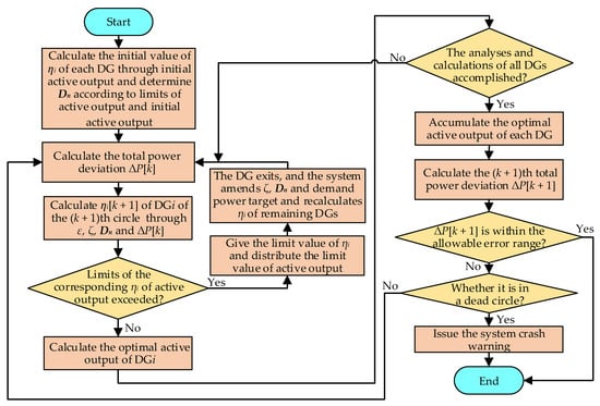
Figure 1.
The flow of the improved pinning consensus algorithm based on ICR.
4. Distributed Hierarchical Optimization Control Method
The traditional centralized control embraces some disadvantages, such as high communication bandwidth requirements and easy communication congestion. In order to tackle the above drawbacks, the hierarchical control architecture adopts the distributed controllers to improve the overall response performance of the system and achieve the autonomous control of each layer.
In the grid-connected AC microgrid, the distributed hierarchical architecture is comprised of a first control layer, a second control layer, and a third control layer. The droop control based on closed-loop feedback of voltage and current is adopted in the first control layer. The optimization control of frequency and voltage is employed by the second control layer to stabilize the frequency and voltage at PCC of the system. The economic optimization operation control is utilized in the third control layer. Simultaneously, the optimal active output reference value of DGs is computed through employing the improved pinning consensus algorithm based on ICR and sent to the P–f droop control loop to reduce the total operation cost of the system. The distributed hierarchical control architecture of the grid-connected microgrid is depicted in Figure 2. The droop control is utilized by each DG in the grid-connected microgrid to guarantee the reasonable distribution of DG output power and the basic stability of frequency and voltage. If the total power generation of DGs in the microgrid is insufficient, the power would be purchased from the grid to jointly supply the power to the load, so as to complete the balance of supply and demand of power, as well as satisfy the requirement of users.
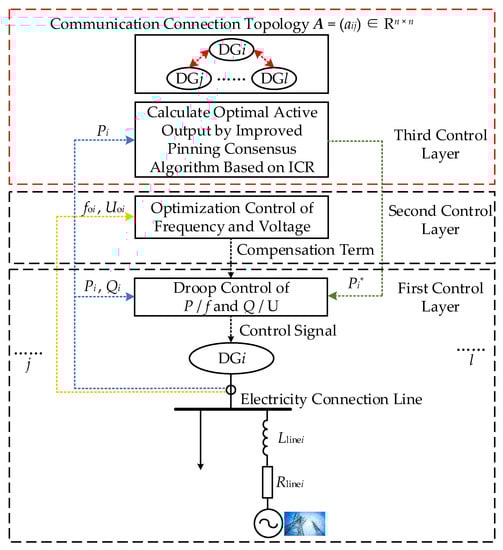
Figure 2.
Distributed hierarchical control architecture of grid-connected microgrids.
For the convenience of research, in this paper, it is assumed that DG grid-connection is the process of connecting photovoltaic generation units to the grid through DC/DC converters and inverters. The primary regulation of frequency and voltage of the power system is simulated by inverters. The active output P of the DG is linearly relevant to the integral of frequency f, of which P is adjusted by changing f. The reactive output Q is linearly related to the voltage difference U–Upcc, so Q can be regulated by altering U [16]. Thus, the droop control of P/f and Q/U is adopted by inverters. The droop control formulas of P/f and Q/U are represented in Equation (21).
where fi, Pi, Ui, and Qi are the frequency (Hz), active output (kW), voltage amplitude (V), and reactive output (kvar) of the output side of the DGi’ inverter, respectively. fi* and Ui* respectively symbolize the reference frequency (Hz) and reference voltage amplitude (V) of DGi. mi and ni are respectively the active droop coefficient (Hz/kW) and reactive droop coefficient (V/kvar) of DGi. Pi* and Qi* respectively indicate the reference active output (kW) and reference reactive output (kvar) of DGi.
The information of frequency and voltage outputted from the grid side of the inverter is collected by the second control layer, which subtracts the corresponding reference value to generate the deviation term later. The compensation term is generated by the deviation through the PI controller and then sent to the first control layer to compensate the frequency and voltage outputted by the droop control loop. The compensation terms of frequency and voltage as well as droop control formulas of P–f and Q–U with compensation terms are shown in Equations (22)–(25). Thereby the fluctuations of frequency and voltage at PCC are eliminated, and the stability of frequency and voltage of the system is improved.
where foi and Uoi are the frequency (Hz) and voltage amplitude (V) outputted from the grid side of the inverter, respectively. ki,f1 and ki,f2 are the proportional coefficient and integral coefficient of the frequency optimization PI controller, respectively. ki,u1 and ki,u2 express the proportional coefficient and integral coefficient of the voltage optimization PI controller, respectively.
For the sake of reducing the total operation cost of the system, the local communication is utilized by DGs in the third control layer to obtain the active output information of adjacent DGs. The active output information is acquired by the sensor and the collected information is transmitted to the processor of DG agents. Based on Equation (13), the ICR is calculated by the processor, and then the updated ICR is computed by employing Equation (18). Finally, Equation (20) is utilized to compute the optimal active output reference value. The optimal active output reference value is emitted to the P–f droop control loop. Afterwards, the droop control is employed to complete the economic distribution of active output of DGs. Accordingly, the grid-connected microgrid system can be in an economic optimization operation state. In addition, the operation cost of each DG and the cost of power purchased from the grid are reduced, and the total power demand of the load is met. With the coordination of the three control layers, the system can rapidly respond to load changes, maintain the stability of frequency as well as voltage, and accomplish the goal of economic optimization.
The factors that affect the control performance and the economic optimization operation state of the system are involved with the grid electricity price, ζ, ε, communication connection topology, and DG plug-and-play.
It can be seen from Equation (8) that the economic optimization operation state of the system is affected by time-of-use price (TOUP) of the whole day. The ICR convergence value of each DG in different periods is changed with the alteration of the grid electricity price. Thus, the optimal active output target, power distribution ratio, active power transmitted by the grid, and the total cost of economic operation are altered.
From Equation (18), the introduction degree of the consensus variable to reference value is changed with the change of ζ, and thus, the calculation rate of consensus variable is influenced. If ζ is too small, it is equivalent to no pinning term, resulting in the reduction of the convergence speed, dynamic performance, and steady-state calculation precision of the algorithm. If ζ is too large, the value of the pinning term is excessively large, the convergence is lost in the algorithm, and the stabilization is lost in the hierarchical control system. Consequently, the appropriate ζ should be ensured to improve the dynamic and steady-state performance of the algorithm and the control performance of economic optimization operation of the system.
Similarly, the response speed of the system to eliminate the total power deviation is altered with the variation of ε, and then the update rate of the consensus variable is affected. The too-small ε makes the power deviation elimination term too small, which lowers the convergence speed and dynamic performance of the algorithm. If ε is enormously large, the dynamic convergence oscillation amplitude of the algorithm would be larger. Simultaneously, the dynamic convergence performance and steady-state calculation precision of the algorithm would be reduced, or the convergence would even be lost. The inappropriate value of ε would reduce the response speed and dynamic control performance of the economic optimization operation of the system, which may make the economic optimization operation of the system invalid and the system unstable, too. Accordingly, the overall performance of the algorithm and the economic optimization control performance of the system could be improved by the appropriate ε.
On the one hand, it can be known from Equation (19) that the communication connection topology of the system is varied with the variation of communication lines between DGs and the joining or exiting of DGs, then the element dij in the row-stochastic matrix Dn is modified. Thus, the convergence speed, dynamic performance, and steady-state precision of the improved pinning consensus algorithm based on ICR are influenced. Likewise, the control performance and the economic optimization operation state of the third control layer are changed. If the condition of the row-stochastic matrix cannot be satisfied through the system Laplace matrix L, the divergency is possessed by the algorithm, and the instability is held by the system. If the communication lines are increased, the algebraic connectivity of the corresponding topology is augmented, and dij is concurrently amended. At this point, the convergence speed and dynamic performance of the algorithm are improved, but the communication cost is ascending. Therefore, it is essential to determine the appropriate communication connection topology in accordance to the actual system configuration. On the other hand, it can be seen from Equation (2) that the active power transmitted from the grid to the microgrid is also altered with the joining or exiting of DGs, which changes the total economic operation cost and the economic optimization operation state of the system.
In addition, it can be known form Equation (18) that the convergence speed of the consensus variable would also be affected by the initial conditions, such as initial ICR and initial active output. Furthermore, the dynamic convergence performance and calculation time of the algorithm would be reduced, the time for the system to eliminate the total power deviation would be increased, and the goal of the economic optimization of the system would be also affected by the improper setting of the initial conditions.
On account of the influence of the ambient temperature (AT) and the characteristics of the conductor, DLR constraint would be generated by the microgrid, thus changing the power flow limits of electric transmission lines of DGs and altering the active output limits of DGs [32]. As can be seen from Equation (13), the ICR of the specific DG and the computation of ICR of other DGs would be changed by the variation of active output of the specific DG, thus changing the optimal active output target of each DG, the output power of the grid, and the total operation cost, which may result in the failure of the system to realize the economic optimization operation.
5. Experiments and Analyses
In this paper, a simulation model of six DG parallel operation systems has been constructed by Matlab/Simulink simulation software to testify the effectiveness and response performance of the economic optimization control method of grid-connected microgrids based on improved pinning consensus. The performance changes before and after the improvement of the algorithm and the impact of different factors on the system have been analysed. The power connection topology and communication connection topology of the system are depicted in Figure 3. The simulation control framework of DGs participating in the economic optimization operation is shown in Figure 4. The rated active power, power limits, initial active power, filter parameters, control parameters, and cost model parameters of each DG are indicated in Table 1. The parameters of the system model are represented in Table 2. In Table 2, the electricity price in the peak period, flat-valley period, and valley period are respectively 6.84 ¥/(kW·h), 6.74 ¥/(kW·h), and 6.70 ¥/(kW·h).
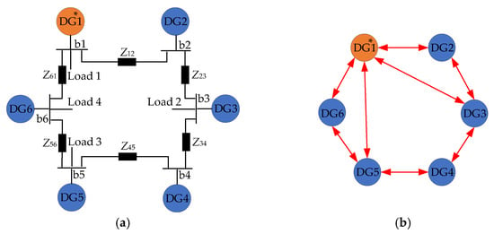
Figure 3.
The power connection topology and communication connection topology of the system: (nodes with * are pinning nodes, the same below) (a) power connection topology; (b) communication connection topology.
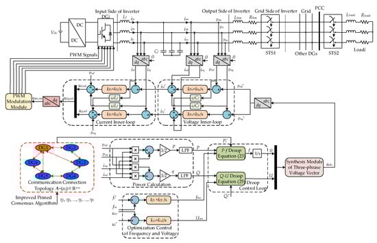
Figure 4.
Simulation control framework of DG participating in economic optimization operation.

Table 1.
Rated active power, power limits, initial active power, filter parameters, control parameters, and cost model parameters of each DG.
Table 2.
Parameters of the system model.
5.1. Comparative Analysis before/after Algorithm Improvement and Research on the Load Response Performance
The algorithm before improvement is calculated by Equation (15), and the improved algorithm proposed in this paper is calculated by Equation (19). The performance changes before and after the algorithm improvement are simulated at first. The change curves of each DG’s ICR, the change curves of each DG’s active output and grid output power, the change curves of the cumulative sum of each DG’s active output and grid output power, and the total demand power before and after algorithm improvement are respectively shown in Figure 5 and Figure 6 (ζ is set as 0.1).
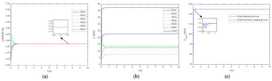
Figure 5.
The change curves of variables of the system before algorithm improvement: (a) change curves of each DG’s ICR; (b) change curves of each DG’s active output and grid output power; (c) change curves of the cumulative sum of each DG’s active output and grid output power as well as total demand power.
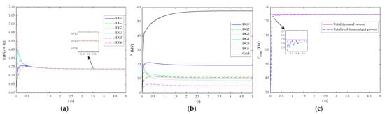
Figure 6.
The change curves of variables of the system after algorithm improvement (ζ is set as 0.1): (a) change curves of each DG’s ICR; (b) change curves of each DG’s active output and grid output power; (c) change curves of the cumulative sum of each DG’s active output and grid output power as well as total demand power.
As can be seen from Figure 5a, the steady-state value of the ICR of each DG before the improvement of the algorithm is 6.766 ¥/(kW·h), which is not identical to the optimal ICR. It takes a long time to realize convergence. Simultaneously, the system cannot achieve the economic optimization operation. It can be seen from Figure 6a that, after the improvement of the algorithm, the ICR of each DG quickly converges to 6.74 ¥/(kW·h). The steady-state calculation precision of ICR is high and the system can enter the economic optimization operation state. Meanwhile, the convergence speed of the improved algorithm is faster. It can be known from Figure 5b and Figure 6b that the system can attain the stability before and after the improvement of the algorithm, but the active output of each DG calculated by the unimproved algorithm is not optimal. As shown in Figure 5c and Figure 6c, although the dynamic overshoot of total real-time output power is relatively large after the improvement of the algorithm, the goal of the economic optimization operation and the supply and demand balance of power can be achieved at the same time. It can be known that the improved algorithm is characteristic of higher steady-state precision and faster convergence speed, which can make the system realize the minimization of operation cost.
For the sake of analyzing the performance changes after the improvement of the algorithm from the perspective of the computational result, the comparison of performance parameters before and after the algorithm improvement is made, as represented in Figure 7. The ICR deviation is defined as the absolute value of the difference between the convergence value of ICR and 6.74 ¥/(kW·h). Similarly, the total power deviation is defined as the absolute value of the difference between total real-time output power and total demand power. (the simulations in this part only study the situation in flat-valley period)
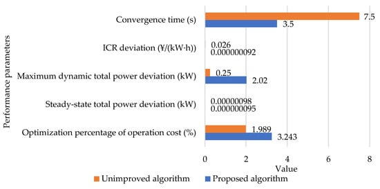
Figure 7.
Comparison of performance parameters before and after algorithm improvement.
As can be seen from Figure 7, the convergence time after the improvement of the algorithm is shortened by about 4 s, and the ICR deviation is approximately zero. With the increase of convergence speed, the maximum dynamic total power deviation is correspondingly larger, but the steady-state total power deviation is smaller. Therefore, the shorter convergence time and higher calculation precision are characteristic of the proposed algorithm, which is conducive to be applied in the actual control system, requiring shorter response time and higher control precision. In the meantime, the total power deviation is eliminated by the method under the premise of minimizing the operation cost.
In order to evaluate the optimization degree of operation cost of the system, the optimization percentage of operation cost is defined as Cop = |Ctb − Cta|/Ctb × 100%, which represents the absolute value of the difference between operation cost before optimization and operation cost after optimization, divided by operation cost before optimization and multiplied by 100%. As depicted in Figure 7, after the improvement of the algorithm, the value of Cop is larger and a higher degree of economic optimization is achieved by the system. Accordingly, the effectiveness of the economic optimization capability of the proposed method is testified. In addition, the power rating of the simulation system model in this paper is kW, but the practical power rating of the urban microgrid is mostly MW or higher. It means that the practical operation cost reduced by the proposed method will be greater and the economic profitability obtained by the power supply company will be higher. Last but not least, the convergence performance of the unimproved algorithm is primarily dependent on the initial conditions, and its economic optimization performance is greatly affected by the initial conditions.
The optimization capability of frequency and voltage of the system adopting the proposed method and the power response characteristics of DGs have been studied. It is assumed that the system responds to loads 1, 2, and 3 at 0 s to achieve the economic optimization operation before 5 s and send the optimal active output target to the droop control layer. Meanwhile, supposing that load 4 begins to operate at 7 s, the optimal active output target is sent to the droop control layer at 12 s. The change curves of each DG’s ICR, the change curves of each DG’s active output and grid output power, and the change curves of the cumulative sum of each DG’s active output and grid output power as well as total demand power under variable load condition are indicated in Figure 8.
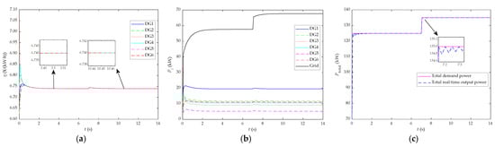
Figure 8.
The change curves of variables of the system under variable load condition: (a) change curves of each DG’s ICR; (b) change curves of each DG’s active output and grid output power; (c) change curves of the cumulative sum of each DG’s active output and grid output power as well as total demand power.
As represented in Figure 8, the system can rapidly respond and tend to be stabilized during 0~3.5 s. After the system is stabilized, the ICR of each DG is converged to 6.74 ¥/(kW·h), and the total power deviation is decreased to zero. The load 4 is put into operation at 7 s and the system quickly responds during 7~10.45 s. In the response process, the ICR of each DG is increased at first and then is decreased, and is finally equivalent to 6.74 ¥/(kW·h), thus reducing the operation cost of DGs. Likewise, the active output of each DG is first augmented suddenly and then decreases. Ultimately, the increased power demand is satisfied by the grid. Meanwhile, in the response process after 7 s, the total real-time output power is slightly fluctuated. It is confirmed that the superior response performance under variable load condition is possessed by the system, which can accomplish the economic optimization operation.
The change curves of output frequency, output voltage amplitude, and the active output at the inverter side of DG1 are depicted in Figure 9. It can be seen from Figure 9a,b that, while the system reacts initially and responds to load 4, the output frequency and output voltage amplitude of DG1 are respectively decreased at first. After the response process of 0.2 s, the optimization control of frequency and voltage takes effect so that the frequency and voltage amplitude are restored to about 50 Hz and 311 V, respectively. During 5~7 s and 12~14 s, the economic optimization operation control makes DG1 perform the optimal active output target and then the active output at inverter side of DG1 is decreased. As a result, the frequency and voltage amplitude of DG1 recover to the reference value after transient fluctuation. After the system is stabilized, the demand power of load 4 is conveyed by the grid.
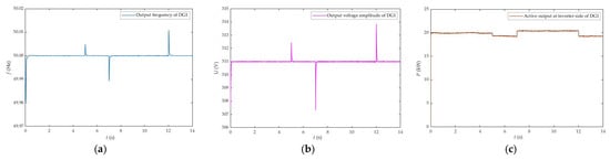
Figure 9.
Change curves of output frequency, output voltage amplitude, active output at inverter side of DG1: (a) change curve of output frequency of DG1; (b) change curve of output voltage amplitude of DG1; (c) change curve of active output at inverter side of DG1.
As it is shown in Figure 9c, because the response bandwidth of droop control is wider than economic optimization operation control, the active output at the inverter side of DG1 is first increased under the role of droop control in the period of 0~5 s. During 5~7 s, the optimal active output target is sent to DG1 by the economic optimization operation control layer and the optimal active output target is executed through the inverter of DG1. The steady-state active output of DG1 tends to be the optimal active output target of 19.51 kW. During 7~12 s, the active output of DG1 is increased on account of rapid response of droop control to satisfy the power demand of load 4. After 12 s, the active output of DG1 is decreased and is finally equivalent to 19.51 kW, approximately. The response processes of the active output of other DGs are similar. As a conclusion, it is verified that the system is characteristic of superior recovery capability of frequency and voltage, better power response capability, faster regulation speed, and higher control accuracy. In addition, the response bandwidth between the economic optimization operation control, optimization control of frequency and voltage, and droop control must be strictly set in the practical application; otherwise, the disturbance signal of active output will be frequently sent to the droop control layer by the economic optimization operation control layer, resulting in the large fluctuation of active output of DGs and the instability of the system.
For the sake of evaluating the performance of optimization control of frequency and voltage as well as power optimization response of DGs, the evaluation indicators such as maximum dynamic frequency deviation ffd = |f − f*|, maximum dynamic voltage deviation UUd = |U − U*|, and maximum dynamic power optimization deviation PPd = |P − P*| are defined, which correspond to the absolute value of the difference between real value and reference value. The smaller value suggests that the better control performance is possessed by the proposed method. The data of DG1 in Figure 9 is employed to compute ffd,1, UUd,1, and PPd,1 of DG1, as shown in Figure 10. ffd,1, UUd,1, and PPd,1 are respectively less than 0.05 Hz, 5 V, and 2%∙P*, which satisfies the basic requirements of control precision in the dynamic process. Additionally, the corresponding steady-state deviations of frequency, voltage, and power optimization of DG1 are approximately zero. It is shown that the control precision of frequency and voltage of the proposed method is higher. Synchronously, the control performance of the inverter of the DG is superior when responding to the active output target. It means that the method could be applied to the practical microgrid system to enhance the economic interest and improve the quality of frequency and voltage.
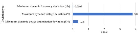
Figure 10.
Maximum dynamic frequency deviation, maximum dynamic voltage deviation and maximum dynamic power optimization deviation of DG1.
5.2. Research on the Effect of TOUP of Whole Day
In this paper, the control performance of the economic optimization operation is principally represented by the dynamic and steady performance of the algorithm. When the economic optimization operation is realized by the system, the ICR of each DG should be converged to the grid electricity price. Nevertheless, there is the TOUP of the whole day mechanism in the actual system. The economic optimization operation state of the grid-connected microgrid would be changed by the mechanism so that the convergence value of ICR and the optimal active output of each DG are different at diverse periods throughout the whole day. Likewise, the total power demand would be varied in the peak period, flat-valley period, and valley period, showing a downward trend. The schematic diagram of TOUP of the whole day is shown in Figure 11. The whole day is segmented into six periods: 0–7 h, 7–9 h, 9–12 h, 12–17 h, 17–22 h, and 22–24 h. The change curves of each DG’s ICR, the change curves of each DG’s active output and grid output power, and the change curves of the cumulative sum of each DG’s active output and grid output power as well as total demand power under TOUP of the whole day and variable load condition are depicted in Figure 12.
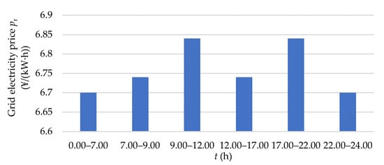
Figure 11.
TOUP of the whole day.
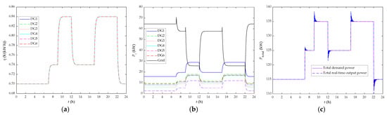
Figure 12.
The change curves of variables of the system under TOUP of the whole day and variable load condition: (a) change curves of each DG’s ICR; (b) change curves of each DG’s active output and grid output power; (c) change curves of the cumulative sum of each DG’s active output and grid output power as well as total demand power.
It can be known from Figure 12 that the system is in the initial zero-response state at 0–7 h and the system is in the stable state before 0 h on account of the constant electricity price. In the remaining five periods, the changes of the electricity price of periods and total demand power are rapidly responded by the ICR and active output of each DG, so that the ICR of each DG is converged to the grid electricity price at diverse periods. Meanwhile, the total operation cost of the system is minimized. After a transient dynamic process, the changed total power demand can be met by the accumulation of the DGs’ active output and grid output power. For example, the ICR of each DG is quickly converged to 6.74 ¥/(kW·h) within 7–9 h, and the total power consumption of 125 kW can be satisfied by active output of each DG and output power of the grid. The dynamic response speed is fast and the overshoot is small, too. As can be seen from Figure 12b, since the total power demand has suddenly increased at the peak period, the active output of each DG is slowly raised. Thus, a reverse-peak regulation has occurred in the output power of the grid to meet the power demand, depicting a tendency of the sudden increase at first and then slow decrease. It is proven that, under the condition of changing electricity price and load changes, the proposed method could quickly obtain the optimal ICR and optimal active output of each DG to realize the economic optimization operation and eliminate the steady-state total power deviation, which makes the microgrid system have superior steady-state control performance.
5.3. Research on the Effect of Pinning Coefficient ζ
The convergence speed of the algorithm can be improved by the pinning term, which makes the ICR of each DG quickly tend to the reference value, so that the optimal active output can be rapidly computed and emitted to the first control layer. The convergence speed, performance, and convergence of the algorithm would be influenced by altering the pinning coefficient. In this paper, the system response experiments have been carried out when ζ is set as 0.01, 0.1, 1, and 10, respectively (the simulations in this part only study the situation in the flat-valley period, the same as below). The change curves of each DG’s ICR, the change curves of each DG’s active output and grid output power, and the change curves of the cumulative sum of each DG’s active output and grid output power as well as total demand power are respectively represented in Figure 6, Figure 13, Figure 14 and Figure 15 when ζ is set as 0.01, 0.1, 1, and 10.
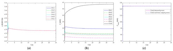
Figure 13.
The change curves of variables of the system when ζ is set as 0.01: (a) change curves of each DG’s ICR; (b) change curves of each DG’s active output and grid output power; (c) change curves of the cumulative sum of each DG’s active output and grid output power as well as total demand power.
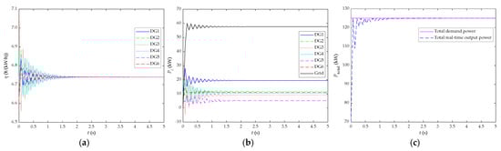
Figure 14.
The change curves of variables of the system when ζ is set as 1: (a) change curves of each DG’s ICR; (b) change curves of each DG’s active output and grid output power; (c) change curves of the cumulative sum of each DG’s active output and grid output power as well as total demand power.
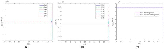
Figure 15.
The change curves of variables of the system when ζ is set as 10: (a) change curves of each DG’s ICR; (b) change curves of each DG’s active output and grid output power; (c) change curves of the cumulative sum of each DG’s active output and grid output power as well as total demand power.
As can be seen from Figure 6, Figure 13, Figure 14 and Figure 15, to set ζ as 0.01, the ICR of each DG is converged to the grid electricity price in the flat-valley period. It takes a long time to realize the economic distribution of the active output. To set ζ as 0.1, the convergence speed of ICR and active output of each DG is accelerated, and the system is stabilized at about 3.5 s. Also, the better overall performance is possessed by the algorithm. Setting ζ as 1, the dynamic response oscillation amplitude of ICR and active output of each DG before convergence and stability become larger. Within 0~1.5 s, the effective active output target cannot be emitted to the first control layer through the layer of economic optimization operation control. After a lengthy dynamic process, the balance of supply and demand of power is completed by the system and the dynamic performance of the algorithm decreases tremendously. Setting ζ as 10, on the one hand, the ICR and active output of each DG are fluctuant and greatly divergent, and the steady-state convergence is not possessed by the algorithm. On the other hand, the instability occurs in the system and the total power demand cannot be met. It can be seen that, only when the value of ζ is appropriate, the faster dynamic convergence speed, better dynamic performance, higher steady-state convergence precision, and application feasibility are held by the algorithm. Through the experimental research, it can be known that when the ζ is greater than 1.12, the convergence is not possessed by the algorithm proposed in the paper, and the balance of supply and demand of the system power cannot be achieved. When the ζ is within 0.5~1, the overall performance of the algorithm becomes superior, with the quick satisfaction of the total power demand of users as well as the realization of the balance of supply and demand of power.
5.4. Research on the Effect of Power Deviation Elimination Term Coefficient ε
The rapid elimination of total power deviation can be attained by the power deviation elimination term. The computation speed of the algorithm is accelerated, which makes the ICR of each DG converge rapidly to the grid electricity price in the flat-valley period. The total power demand would be conjointly met by the calculated optimal active output and active power transmitted from the grid. The convergence speed, performance, and convergence of the algorithm are affected by changing ε. In this paper, ε has been increased by 5 times, 10 times, and 100 times respectively to study the dynamic and steady-state performance of the algorithm. The change curves of each DG’s ICR, the change curves of each DG’s active output and grid output power, and the change curves of the cumulative sum of each DG’s active output and grid output power as well as total demand power are respectively indicated in Figure 16, Figure 17 and Figure 18 when ε is increased by 5 times, 10 times, and 100 times.
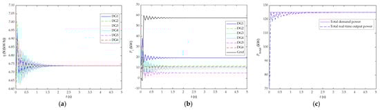
Figure 16.
The change curves of variables of the system when ε is increased by 5 times: (a) change curves of each DG’s ICR; (b) change curves of each DG’s active output and grid output power; (c) change curves of the cumulative sum of each DG’s active output and grid output power as well as total demand power.
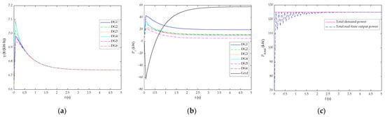
Figure 17.
The change curves of variables of the system when ε is increased by 10 times: (a) change curves of each DG’s ICR; (b) change curves of each DG’s active output and grid output power; (c) change curves of the cumulative sum of each DG’s active output and grid output power as well as total demand power.
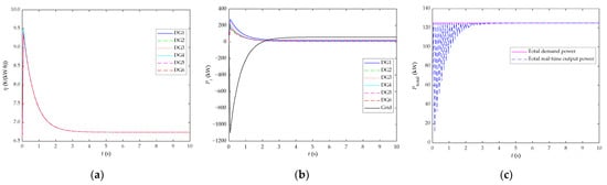
Figure 18.
The change curves of variables of the system when ε is increased by 100 times: (a) change curves of each DG’s ICR; (b) change curves of each DG’s active output and grid output power; (c) change curves of the cumulative sum of each DG’s active output and grid output power as well as total demand power.
As can be seen from Figure 16a,b and Figure 17a,b, when ε is increased by 5 times, the oscillation amplitude and frequency of ICR and active output of each DG are respectively larger and higher during the dynamic response process. The active output of DG3 and DG4 is undulatory violently within 0~1.5 s. The effective active output target is not sent to the first control layer by the economic optimization operation control layer, and the dynamic performance of the algorithm is immensely declined. When ε is increased by 10 times, the oscillation amplitude of ICR and active output of each DG before convergence and stabilization is bigger. Simultaneously, the convergence time is augmented to 4.5 s, but the oscillation frequency is decreased compared with ε increased by 5 times. It can be known that, if ε is too large, the dynamic convergence performance of the algorithm will be decreased and the convergence time will be increased. As can be seen from Figure 16c and Figure 17c, with the enormously big ε, the performance of the algorithm proposed in this paper will be vastly reduced and the active output will be fluctuant immensely. Nevertheless, because of the support of the grid, the total power demand of 125 kW can still be satisfied, and the balance of the supply and demand of the system power is achieved with the small steady-state total power deviation.
As can be seen from Figure 18a,b, with the further increase of ε, the maximum dynamic oscillation amplitude of ICR and optimal active output of each DG is raised and the time to converge to stability is approximately 4.5 s. The superior convergence performance is held by the algorithm, whereas the enormous impact on the grid is caused by the large amplitude oscillation of active output of DGs and the active power conveyed from the grid is variable hugely, which makes the flow power at PCC section unsteady. However, the system stabilization and superior control effect can be attained in the practical application only when setting properly protocol parameters.
5.5. Research on the Effect of Communication Topology Change
The communication topology when DG6 exits is indicated in Figure 19a. The change curves of each DG’s ICR and the change curves of each DG’s active output and grid output power when DG6 exits the communication topology is shown in Figure 19b,c.
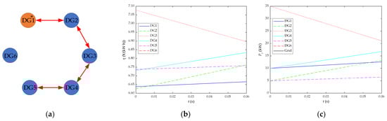
Figure 19.
Communication topology and change curves of variables of the system when DG6 exits the communication topology: (a) communication topology when DG6 exits; (b) change curves of each DG’s ICR; (c) change curves of each DG’s active output and grid output power.
It can be seen from Figure 19b,c that the condition of the row-stochastic matrix is not met by the matrix L on account of DG6’s exiting from the communication topology, and that DG6 cannot participate in the calculation, resulting in no change curves. The ICR and active output of other DGs are divergent immensely and the system becomes unstable. In addition, the total power demand is not met through the active output of each DG and output power of the grid.
The communication topologies of low algebraic connectivity and high algebraic connectivity are shown in Figure 20. The change curves of each DG’s ICR, the change curves of each DG’s active output and grid output power, and the change curves of the cumulative sum of each DG’s active output and grid output power as well as total demand power under the communication topologies of low algebraic connectivity and high algebraic connectivity are respectively depicted in Figure 21 and Figure 22.
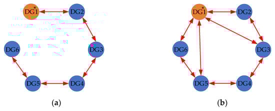
Figure 20.
Communication topologies of low algebraic connectivity and high algebraic connectivity: (a) communication topology of low algebraic connectivity; (b) communication topology of high algebraic connectivity.
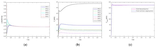
Figure 21.
Change curves of variables of the system under the communication topology of low algebraic connectivity: (a) change curves of each DG’s ICR; (b) change curves of each DG’s active output and grid output power; (c) change curves of the cumulative sum of each DG’s active output and grid output power as well as total demand power.
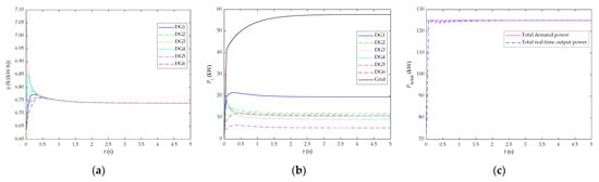
Figure 22.
Change curves of variables of the system under the communication topology of high algebraic connectivity: (a) change curves of each DG’s ICR; (b) change curves of each DG’s active output and grid output power; (c) change curves of the cumulative sum of each DG’s active output and grid output power as well as total demand power.
It can be seen from Figure 19, Figure 21 and Figure 22 that the ICR of each DG is rapidly converged to the optimal ICR by right of the improved pinning consensus algorithm based on ICR, which is identical to the grid electricity price in the flat-valley period. Thus, the total operation cost of the grid-connected microgrid system is minimized. Additionally, the economic distribution of active output is realized by each DG. The power of DGs is supplied to the load together with the grid power, thus meeting the total power demand of users of 125 kW. The simulation results have shown that the superior dynamic and steady-state control performance is possessed by the system when the condition of the row-stochastic matrix is satisfied by the corresponding L of the communication topology and the algebraic connectivity of the communication topology is higher. Simultaneously, the pinning term of the algorithm keeps the response speed of the system correspondingly fast, even if the algebraic connectivity of the communication topology is low. It implies that the reduction of communication construction cost and superior control effect will be achieved in the practical application.
5.6. Research on the Effect of DG Plug-of-Play
The change curves of each DG’s ICR, the change curves of each DG’s active output and grid output power, and the change curves of the cumulative sum of each DG’s active output and grid output power as well as total demand power when the DG joins and exits are shown in Figure 23 and Figure 24, respectively.
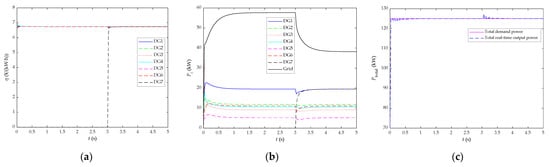
Figure 23.
Change curves of variables of the system when the DG joins: (a) change curves of each DG’s ICR; (b) change curves of each DG’s active output and grid output power; (c) change curves of the cumulative sum of each DG’s active output and grid output power as well as total demand power.
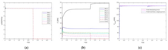
Figure 24.
Change curves of variables of the system when the DG exits: (a) change curves of each DG’s ICR; (b) change curves of each DG’s active output and grid output power; (c) change curves of the cumulative sum of each DG’s active output and grid output power as well as total demand power.
As can be seen from Figure 23, during 0~3 s, six DGs operate in parallel, which realizes the goal of the economic optimization operation of the system. The ICR of each DG is converged to consistency, which is equivalent to the grid electricity price in the flat-valley period. The economic distribution is achieved by the active output of each DG and output power transmitted from the grid, thus satisfying the power demand of 125 kW. During 3~5 s, DG7 takes part in the system operation. The ICR of DG7 is raised continuously and is converged finally, which is corresponding to the grid electricity price in the flat-valley period. In the meantime, the ICR of DG1~6 is declined at first and then is increased, finally identical with the grid electricity price in the flat-valley period. Similarly, the active output of DG1~6 is decreased at first and then is increased with the stable convergence in the end. After DG7 participation in the operation, the active power transmitted from the grid is decreased. In the economic optimization response process after 3 s, the total active output of each DG and grid is fluctuant marginally. Thus, the goal of economic optimization operation, as well as the balance of supply and demand of power, are completed after short-time response.
As can be seen from Figure 24, during 3~5 s, the DG6 withdraws the system operation and the ICR of DG6 tends to be zero quickly. The ICR of DG1~5 is raised at first and is decreased later, which finally converges to the grid electricity price in the flat-valley period. Likewise, the active output of DG1~5 is increased at first and then is reduced. After DG6 withdraws the operation, the active power conveyed from the grid is ascendant. Ultimately, the economic distribution of active output is attained. In the economic optimization response process after 3 s, the fluctuation of total active output of each DG and grid is decreased rapidly. After a short-time response process, the stability is obtained and the total power elimination is quickly eliminated by the system, which meets the power demand and minimizes the total operation cost.
The steady-state optimal active output of each DG when the DG takes part in the operation or withdraws the operation are displayed in Figure 25 and Figure 26, respectively. It can be known that the plug-and-play function of DGs of microgrids can be realized by the proposed control method. When the DG takes part in the operation or withdraws the operation, the response speed of active output is faster, and the overshoot is small. Meanwhile, the ICR consensus and the goal of economic optimization operation of the system are accomplished quickly and the steady-state control precision of the system is higher.
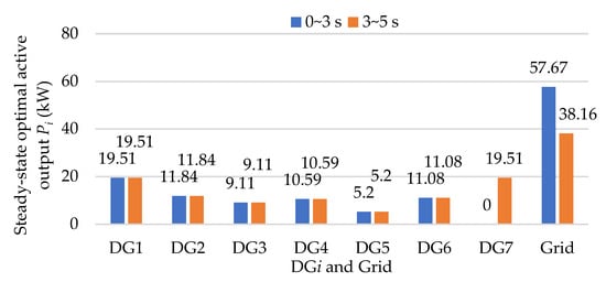
Figure 25.
Comparison of steady-state optimal active output of each DG before and after the joining of DG7.
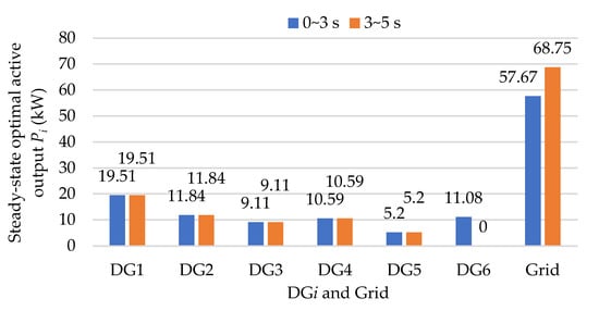
Figure 26.
Comparison of steady-state optimal active output of each DG before and after the exiting of DG6.
5.7. Research on the Effect of Initial Condition
In this paper, the response experiments of the system have been conducted when setting the initial active output at zero and then setting both the initial ICR and initial active output at zero. The change curves of each DG’s ICR, the change curves of each DG’s active output and grid output power, and the change curves of the cumulative sum of each DG’s active output and grid output power as well as total demand power are respectively described in Figure 27 and Figure 28 when the initial active output is set at zero and both the initial ICR and the initial active output are set at zero.
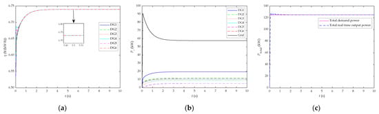
Figure 27.
The change curves of variables of the system when the initial active output is set at zero: (a) change curves of each DG’s ICR; (b) change curves of each DG’s active output and grid output power; (c) change curves of the cumulative sum of each DG’s active output and grid output power as well as total demand power.
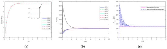
Figure 28.
The change curves of variables of the system when both the initial ICR as well as initial active output are set at zero: (a) change curves of each DG’s ICR; (b) change curves of each DG’s active output and grid output power; (c) change curves of the cumulative sum of each DG’s active output and grid output power as well as total demand power.
By comparing Figure 6 and Figure 27, it can be seen that the ICR of each DG can be eventually converged to the optimal ICR when setting the initial active output at zero. However, the convergence time is increased by about 2 s compared with the condition that the initial conditions are not set to zero. Simultaneously, it takes a long time for the active output of each DG to achieve the stabilization, resulting in a bigger overshoot of the grid output power and a small overshoot of the total real-time output power. As indicated in Figure 28, when both the initial ICR and initial active output are set to zero, the time for the ICR of each DG to attain stability is augmented to 8 s and a larger reverse overshoot occurs in the active output of each DG and the grid. Meanwhile, the optimal active output target calculated within 0~1.75 s is invalid. There is a great overshoot in the total real time output power, and it takes a long time for the system to eliminate the total power deviation. As a conclusion, if the initial conditions are set irrationally, the convergence performance of the algorithm will be sharply decreased, which will make the time required for the system to achieve economic optimization operation, as well as the balance of supply and demand, be increased. It means that the better response effect would be possessed by the system when utilizing the droop control to realize stable operation at first and then carrying out the economic optimization.
5.8. Research on the Effect of DLR
The changes of active output of each DG and the grid as well as the change of economic optimization operation state of the system under DLR constraint have been researched. The communication topology of the system under DLR constraint and change curves of AT of each DG is shown in Figure 29. Assuming that load 4 is put into operation within 12~15 h on a certain day in summer and the AT of DG1 surpasses thirty degrees Celsius, DG1 is subjected to DLR constraint and the upper limit of power flow of transmission line of DG1 is restricted to 18 kW. Because DG1 exceeds the power limit, the proposed algorithm would make DG1 withdraw the communication topology connection, and DG1 would not participate in the ICR calculation. The change curves of each DG’s ICR, the change curves of each DG’s active output and grid output power, and the change curves of the cumulative sum of each DG’s active output and grid output power, as well as total demand power under DLR constraint, are represented in Figure 30.
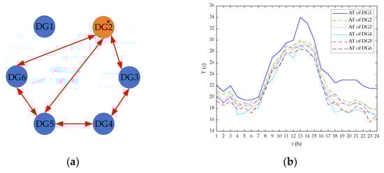
Figure 29.
Communication topology of the system under DLR constraint and changes curves of AT of each DG: (a) communication topology of the system under DLR constraint; (b) change curves of AT of each DG.
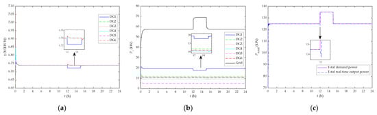
Figure 30.
The change curves of variables of the system under DLR constraint: (a) change curves of each DG’s ICR; (b) change curves of each DG’s active output and grid output power; (c) change curves of the cumulative sum of each DG’s active output and grid output power as well as total demand power.
As it is shown in Figure 30, the system performs the economic optimization response and achieves the stability within 0~12 h. Similarly, the ICR and active output of each DG, as well as the grid output power, tends to be stable, which enables the total power deviation to be eliminated to zero. During 12~15 h, the active output of DG1 is limited to 18 kW and the ICR is decreased to 6.724 ¥/(kW·h) due to DLR constraint. In the response process to load 4, the ICR and active output of other DG are increased in the beginning and then is decreased, and is finally recovered to the steady-state value during 0~12 h. At the same time, the total real-time output power is lessened at first and then is boosted, and is eventually identical to the total demand power. At this moment, the power demand of load 4 is assigned to the grid. During 15~24 h, on account of the exiting of load 4, DG1 is not within DLR constrains, which rejoin the communication topology connection and take part in the economic optimization operation. After the dynamic response process, the ICR and active output of each DG are steady and are restored to the optimal steady-state value during 0~12 h. Meanwhile, the operation cost is reduced and the total power demand is satisfied by the system. It can be known that, under specific DLR constraints, the system cannot enter the optimal economic operation state by employing the proposed method. However, the operation cost of the DG that is not subjected to DLR constraint can still be cut down.
6. Discussions
The research goal of this paper is that the improved pinning consensus algorithm is firstly designed to quickly tackle the economic optimization model of grid-connected microgrids, thus reducing the operation cost of microgrids. Secondly, a distributed three-layer control architecture is established to achieve the rapid response of DGs to load changes and optimize the active output. Simultaneously, the stability of output frequency and voltage is maintained. As can be seen from Figure 5, Figure 6 and Figure 7, in contrast with the unimproved algorithm, the convergence speed of the proposed algorithm is faster. The calculation completion time is less than 3.5 s when setting the parameters reasonably. Concurrently, the calculation precision of ICR and active output, as well as total power, is higher and the maximum steady-state deviation is less than 1 × 10⁻⁷. In addition, the active output of DGs can be economically optimized by the system, which can reduce the total operation cost by about 3.243% and satisfy the needs of transmission loss power and load power. It can be known from Figure 10 that ffd,1, UUd,1, and PPd,1 of DG1 were 0.0199 Hz, 3.8 V, and 0.35 kW, respectively, all of which are less than the corresponding allowable error values, and the steady-state deviation is zero. It is shown that the better capability of frequency and voltage control is possessed by the system, thus achieving the accurate control of active output. The method can realize that the actual control system is characteristic of better response performance, which is conducive to be applied in practical microgrid engineering.
As can be known from the simulation results of Section 5.2, Section 5.6, and Section 5.8, under the influences of TOUP, DG plug-and-play, and DLR constraint, the reduction of operation cost as well as the balance of supply and demand can be realized by the proposed method, thus making the system hold the superior overall response performance. However, for the proposed method, in practical application, it is firstly essential that the response bandwidth between the three control layers should be strictly set, and the response bandwidth from the first control layer to the third control layer should be gradually reduced to realize the stable operation of the system; otherwise, the control would be noneffective. Secondly, in accordance to the simulation results of Section 5.3, Section 5.4, Section 5.5 and Section 5.7, it can be seen that the proposed algorithm achieves the convergence and fast responsiveness only when the protocol parameters, communication topologies, and initial conditions are reasonably set in the practical application. Thereby, the goals of the stability of the system, the reduction of operation cost, the satisfaction of total power demand, the quality optimization of frequency and voltage, and the accurate control of active output of DGs can be achieved by the proposed method.
On the one hand, the minute-level real-time TOUP model has not been considered and its in-depth influence on the economic optimization model has not been analyzed in this paper. On the other hand, only the alterations of response performance and operation state of the system under hypothetical DLR constraint have been studied. Furthermore, there is also no specific mathematical model based on the DLR effect to deeply analyse the in-depth influence of multiple factors such as weather conditions and conductor parameters on the economic optimization operation of the system, which will be further studied in the future.
7. Conclusions
An improved pinning consensus algorithm based on ICR has been designed in this paper, which can optimize the operation cost of grid-connected microgrids. Meanwhile, the optimal ICR and active output of DGs can be calculated by the algorithm in a short time, and the steady-state calculation deviation is extremely small, which can make the system quickly enter the economic optimization operation state. In addition, under the influences of TOUP, DG plug-and-play, DLR constraint, and other factors, the proposed algorithm still is characteristic of superior performance and can reduce the operation cost of each DG. Subsequently, an economic optimization control method of grid-connected microgrids based on improved pinning consensus has been proposed and a distributed three-layer control architecture has been constructed. By employing the method, the economic profitability of microgrids is increased. Similarly, the output frequency and voltage of DGs can be rapidly restored to the rated value. By the droop control, load changes can be quickly responded to meet the total demand power and realize the economic allocation of active power output. Eventually, the validity of the proposed method has been verified through simulation experiments. The changes of convergence performance before and after the improvement of the algorithm have been analyzed comparatively. Additionally, the effects of protocol parameters, communication topology, and initial conditions on the response performance of the method have been simulated and researched. It has been confirmed that the power demand and the requirement of power quality for users can be met by the method, as well on the premise of achieving the goal of economic optimization.
Author Contributions
Conceptualization, Z.T.; methodology, Z.T.; software, Z.T., C.Z. and S.W.; validation, Z.T., C.Z. and S.W.; formal analysis, H.L.; investigation, X.W.; resources, C.Z. and X.W.; writing—original draft, Z.T. and C.Z.; writing—review and editing, C.Z., S.W. and P.G.; visualization, Z.T., P.G. and H.L.; supervision, P.G. and H.L.; funding acquisition, X.W. All authors have read and agreed to the published version of the manuscript.
Funding
This work was partly funded by the National Nature Science Foundation of China, grant number 61873294 and fully funded by the Quality Engineering Project Foundation of Postgraduate Education of Anhui Province of China, grant number 2022xscx094.
Data Availability Statement
Not applicable.
Acknowledgments
The authors wish to thank the respected editors and reviewers for contributing their valuable time, pertinent and precious suggestions that have helped advance the quality of the study.
Conflicts of Interest
The authors declare no conflict of interest.
Abbreviations
| AT | Ambient Temperature |
| BESS | Battery Energy Storage System |
| DG | Distributed Generation |
| DLR | Dynamic Line Rating |
| ETESs | Electric-Thermal Energy Storages |
| ICR | Incremental Cost Rate |
| MAS | Multi-Agent System |
| TOUP | Time-of-Use Price |
References
- Wang, J.J.; Dong, C.Y.; Jin, C. Distributed Uniform Control for Parallel Bidirectional Interlinking Converters for Resilient Operation of Hybrid AC/DC Microgrid. IEEE Trans. Sustain. Energy 2022, 13, 3–13. [Google Scholar]
- Jabr, R.A. Economic Operation of Droop-Controlled AC Microgrids. IEEE Trans. Power Syst. 2022, 37, 3119–3128. [Google Scholar] [CrossRef]
- Chen, C.; Duan, S. Microgrid Economic Operation Considering Plug-in Hybrid Electric Vehicles Integration. J. Mod. Power Syst. Clean Energy 2015, 3, 221–231. [Google Scholar] [CrossRef]
- Nisha, K.S.; Gaonkar, D.N. Model Predictive Controlled Three-Level Bidirectional Converter with Voltage Balancing Capability for Setting up EV Fast Charging Stations in Bipolar DC Microgrid. Electr. Eng. 2022, 104, 2653–2665. [Google Scholar] [CrossRef]
- Zhang, J.; Qin, D.; Ye, Y. Multi-Time Scale Economic Scheduling Method Based on Day-Ahead Robust Optimization and Intraday MPC Rolling Optimization for Microgrid. IEEE Access 2021, 9, 140315–140324. [Google Scholar] [CrossRef]
- Dey, B.; Basak, S.; Pal, A. Demand-Side Management Based Optimal Scheduling of Distributed Generators for Clean and Economic Operation of a Microgrid System. Int. J. Energy Res. 2022, 46, 8817–8837. [Google Scholar] [CrossRef]
- Akbari, R.; Tajalli, S.Z.; Kavousi-Fard, A. Economic Operation of Utility-Connected Microgrids in a Fast and Flexible Framework Considering Non-Dispatchable Energy Sources. Energies 2022, 15, 2894. [Google Scholar]
- Lyu, C.; Jia, Y.; Xu, Z. A Novel Communication-Less Approach to Economic Dispatch for Microgrids. IEEE Trans. Smart Grid 2021, 12, 901–904. [Google Scholar] [CrossRef]
- Zhao, C.; Sun, W.; Wang, J.; Fang, Z. Distributed Robust Secondary Voltage Control for Islanded Microgrid with Nonuniform Time Delays. Electr. Eng. 2021, 103, 2625–2635. [Google Scholar]
- Li, Y.; Yang, Z.; Li, G.; Zhao, D.; Tian, W. Optimal Scheduling of an Isolated Microgrid with Battery Storage Considering Load and Renewable Generation Uncertainties. IEEE Trans. Ind. Electron. 2019, 66, 1565–1575. [Google Scholar] [CrossRef]
- Harsh, P.; Das, D. Optimal Coordination Strategy of Demand Response and Electric Vehicle Aggregators for the Energy Management of Reconfigured Grid-Connected Microgrid. Renew. Sustain. Energy Rev. 2022, 160, 112251. [Google Scholar] [CrossRef]
- Zhang, Y.; Liang, C.; Shi, J.; Lim, G.; Wu, Y. Optimal Port Microgrid Scheduling Incorporating Onshore Power Supply and Berth Allocation Under Uncertainty. Appl. Energy 2022, 313, 118856. [Google Scholar] [CrossRef]
- Yang, M.; Cui, Y.; Wang, J. Multi-Objective Optimal Scheduling of Island Microgrids Considering the Uncertainty of Renewable Energy Output. Int. J. Electr. Power Energy Syst. 2023, 144, 108619. [Google Scholar] [CrossRef]
- Das, D.; Hossain, M.J.; Mishra, S. Bidirectional Power Sharing of Modular Dabs to Improve Voltage Stability in DC Microgrids. IEEE Trans. Ind. Appl. 2022, 58, 2369–2377. [Google Scholar] [CrossRef]
- Pham, X.H.T. An Improved Controller for Reactive Power Sharing in Islanded Microgrid. Electr. Eng. 2021, 103, 1679–1689. [Google Scholar] [CrossRef]
- Alghamdi, B.; Claudio, C. Frequency and Voltage Coordinated Control of a Grid of AC/DC Microgrids. Appl. Energy 2022, 310, 118427. [Google Scholar] [CrossRef]
- Dashtaki, A.A.; Hakimi, S.M.; Hasankhani, A.; Derakhshani, G.; Abdi, B. Optimal Management Algorithm of Microgrid Connected to the Distribution Network Considering Renewable Energy System Uncertainties. Int. J. Electr. Power Energy Syst. 2023, 145, 108633. [Google Scholar] [CrossRef]
- Guo, J.; Meng, Z.; Chen, Y. Harmonic Transfer-Function-Based αβ-Frame SISO Impedance Modeling of Droop Inverters-Based Islanded Microgrid with Unbalanced Loads. IEEE Trans. Ind. Electron. 2023, 70, 452–464. [Google Scholar] [CrossRef]
- Wang, Z.; Chen, Y.; Li, X. Adaptive Harmonic Impedance Reshaping Control Strategy Based on a Consensus Algorithm for Harmonic Sharing and Power Quality Improvement in Microgrids with Complex Feeder Networks. IEEE Trans. Smart Grid 2022, 13, 47–57. [Google Scholar] [CrossRef]
- Dabbaghjamanesh, M.; Kavousi-Fard, A.; Mehraeen, S.; Zhang, J.; Yang Dong, Z. Sensitivity Analysis of Renewable Energy Integration on Stochastic Energy Management of Automated Reconfigurable Hybrid AC-DC Microgrid Considering DLR Security Constraint. IEEE Trans. Ind. Inf. 2020, 16, 120–131. [Google Scholar] [CrossRef]
- Mohammed, N.; Lashab, A.; Ciobotaru, M.; Guerrero, J.M. Accurate Reactive Power Sharing Strategy for Droop-Based Islanded AC Microgrids. IEEE Trans. Ind. Electron. 2023, 70, 2696–2707. [Google Scholar] [CrossRef]
- Tightiz, L.; Yang, H.; Bevrani, H. An Interoperable Communication Framework for Grid Frequency Regulation Support from Microgrids. Sensors 2021, 21, 4555. [Google Scholar] [CrossRef] [PubMed]
- Dabbaghjamanesh, M.; Wang, B.; Kavousi-Fard, A.; Hatziargyriou, N.D.; Zhang, J. Blockchain-Based Stochastic Energy Management of Interconnected Microgrids Considering Incentive Price. IEEE Trans. Control. Netw. Syst. 2021, 8, 1201–1211. [Google Scholar] [CrossRef]
- Bucolo, M.; Buscarino, A.; Famoso, C.; Fortuna, L. Chaos Addresses Energy in Networks of Electrical Oscillators. IEEE Access 2021, 9, 153258–153265. [Google Scholar] [CrossRef]
- Zuo, K.; Wu, L. Enhanced Power and Energy Coordination for Batteries under the Real-Time Closed-Loop, Distributed Microgrid Control. IEEE Trans. Sustain. Energy 2022, 13, 2027–2040. [Google Scholar] [CrossRef]
- Ali, S.; Kazmi, S.A.A.; Malik, M.M. Energy Management in High RER Multi-Microgrid System via Energy Trading and Storage Optimization. IEEE Access 2022, 10, 6541–6554. [Google Scholar] [CrossRef]
- Dong, H.; Fu, Y.; Jia, Q.; Wen, X. Optimal Dispatch of Integrated Energy Microgrid Considering Hybrid Structured Electric-Thermal Energy Storage. Renew. Energy 2022, 199, 628–639. [Google Scholar] [CrossRef]
- Li, L.; Han, Y.; Li, Q.; Pu, Y.; Sun, C.; Chen, W. Event-Triggered Decentralized Coordinated Control Method for Economic Operation of an Islanded Electric-Hydrogen Hybrid DC Microgrid. J. Energy Storage 2022, 45, 103704. [Google Scholar] [CrossRef]
- Wang, H.; Li, W.; Yue, Y.; Zhao, H. Distributed Economic Control for AC/DC Hybrid Microgrid. Electronics 2022, 11, 13. [Google Scholar] [CrossRef]
- Jiang, K.; Wu, F.; Zong, X.; Shi, L.; Lin, K. Distributed Dynamic Economic Dispatch of an Isolated AC/DC Hybrid Microgrid Based on a Finite-Step Consensus Algorithm. Energies 2019, 12, 4637. [Google Scholar] [CrossRef]
- Maslak, G.; Orlowski, P. Microgrid Operation Optimization Using Hybrid System Modeling and Switched Model Predictive Control. Energies 2022, 15, 833. [Google Scholar] [CrossRef]
- Dabbaghjamanesh, M.; Kavousi-Fard, A.; Mehraeen, S. Effective Scheduling of Reconfigurable Microgrids With Dynamic Thermal Line Rating. IEEE Trans. Ind. Electron. 2018, 66, 1552–1564. [Google Scholar] [CrossRef]
- Su, W.; Yu, S.S.; Li, H.; Iu, H.H.-C.; Fernando, T. An MPC-Based Dual-Solver Optimization Method for DC Microgrids with Simultaneous Consideration of Operation Cost and Power Loss. IEEE Trans. Power Syst. 2021, 36, 936–947. [Google Scholar] [CrossRef]
- Tao, H.; Zhou, L.; Hao, S.; Paszke, W.; Yang, H. Output Feedback Based PD-Type Robust Iterative Learning Control for Uncertain Spatially Interconnected Systems. Int. J. Robust Nonlinear Control 2021, 31, 5962–5983. [Google Scholar] [CrossRef]
- Wei, J.; Tao, H.; Hao, S.; Paszke, W.; Gałkowski, K. Output Feedback Based Robust Iterative Learning Control via a Heuristic Approach for Batch Processes with Time-Varying State Delays and Uncertainties. J. Process Control. 2022, 116, 159–171. [Google Scholar] [CrossRef]
- Zhuang, Z.; Tao, H.; Chen, Y.; Stojanovic, V.; Paszke, W. An Optimal Iterative Learning Control Approach for Linear Systems with Nonuniform Trial Lengths Under Input Constraints. IEEE Trans. Syst. Man. Cybern. Syst. 2022, 1–13. [Google Scholar] [CrossRef]
- Zhou, L.; Tao, H.; Paszke, W.; Stojanovic, V.; Yang, H. PD-Type Iterative Learning Control for Uncertain Spatially Interconnected Systems. Mathematics 2020, 8, 1528. [Google Scholar] [CrossRef]
- Wang, P.; Chen, W.; Lin, S.; Liu, L.; Sun, Z.; Zhang, F. Consensus Algorithm Based on Verifiable Quantum Random Numbers. Int. J. Intell. Syst. 2022, 37, 6857–6876. [Google Scholar] [CrossRef]
- Olfati-Saber, R.; Murray, R.M. Consensus Problems in Networks of Agents with Switching Topology and Time-Delays. IEEE Trans. Autom. Control 2004, 49, 1520–1533. [Google Scholar] [CrossRef]
Disclaimer/Publisher’s Note: The statements, opinions and data contained in all publications are solely those of the individual author(s) and contributor(s) and not of MDPI and/or the editor(s). MDPI and/or the editor(s) disclaim responsibility for any injury to people or property resulting from any ideas, methods, instructions or products referred to in the content. |
© 2023 by the authors. Licensee MDPI, Basel, Switzerland. This article is an open access article distributed under the terms and conditions of the Creative Commons Attribution (CC BY) license (https://creativecommons.org/licenses/by/4.0/).