A Three-Stage Model to Manage Energy Communities, Share Benefits and Provide Local Grid Services

Abstract

This paper proposes a three-stage model for managing energy communities for local energy sharing and providing grid flexibility services to tackle local distribution grid constraints. The first stage addresses the minimization of each prosumer’s individual energy bill by optimizing the schedules of their flexible resources. The second stage optimizes the energy bill of the whole energy community by sharing the prosumers’ energy surplus internally and re-dispatching their batteries, while guaranteeing that each prosumer’s new energy bill is always be equal to or less than the bill that results for this prosumer from stage one. This collective optimization is designed to ensure an additional collective benefit, without loss for any community member. The third stage, which can be performed by the distribution system operator (DSO), aims to solve the local grid constraints by re-dispatching the flexible resources and, if still necessary, by curtailing local generation or consumption. Stage three minimizes the impact on the schedule obtained at previous stages by minimizing the loss of profit or utility for all prosumers, which are furthermore financially compensated accordingly. This paper describes how the settlement should be performed, including the allocation coefficients to be sent to the DSO to determine the self-consumed and supplied energies of each peer. Finally, some case studies allow an assessment of the performance of the proposed methodology. Results show, among other things, the potential benefits of allowing the allocation coefficients to take negative values to increase the retail market competition; the importance of stage one or, alternatively, the need for a fair internal price to avoid unfair collective benefit sharing among the community members; or how stage three can effectively contribute to grid constraint solving, profiting first from the existing flexible resources.

1. Introduction

Energy communities and collective self-consumption schemes are gaining relevance as national regulations transpose the EU directives and final consumers become more actively involved in the energy generation and supply processes. EU Directive 2018/2001 [1] provides the guidelines that EU member states must follow in their national legislations, by defining the concepts and roles of individual self-consumption (ISC), collective self-consumption (CSC) and renewable energy communities (REC), highlighting the concept of peer-to-peer (P2P) direct trading between local market participants. National regulations are transposing this directive in different ways, as it is for example the cases of Spain and Portugal analyzed in [2]. In the case of Portugal, the regulation for the National Electric System organization and functioning rules includes new rules for the ISC, CSC, REC and citizen energy communities (CEC) [3].

Energy management systems for energy communities have been often addressed in the literature. For example, [4] proposes a model to schedule shiftable loads according to the internal price, which is computed based on the internal supply and demand ratio (SDR), with all prosumers having the same retail and feed-in tariffs (otherwise the SDR is not well defined). First, for each delivery time, the community manager determines the selling and buying prices according to the SDR pricing and to the selling or buying position of the prosumer. Then, each prosumer minimizes its energy bill including an inconvenience cost for shifting load, leading to an equilibrium problem which is solved iteratively. The work in [5] proposes a two-stage model to minimize the energy costs of an REC by centrally scheduling the batteries of its members. In the first stage, the energy bill of the community is minimized by continuously optimizing the batteries’ schedules for a rolling horizon (as described later) to produce the batteries’ setpoint for the next delivery time. In the second stage, setpoints are adapted to always charge when there is an energy surplus of the REC, and discharge when there is an energy deficit. As in the previous work, they also base the internal pricing mechanism on the SDR. The work in [6] focuses on a P2P market structure considering dynamic retail electricity prices to automatically generate bids in a community. In addition to SDR, the authors also compare the effectiveness of Double Auction (DA) and Mid-Market Rate (MMR) pricing models.

In [7], the batteries’ schedules of the members of a microgrid are optimized to reduce the microgrid energy exchange losses by minimizing the power at its interconnection with the main grid. A genetic algorithm is used and compared with classical optimization. An integrated model considering a local energy market, residual balancing and ancillary service mechanisms is proposed in [8], where the provision of flexibility for the utility requires adjustments in the balancing position of each peer according to their traded schedule. This transfer of energy between the balance responsible parties (BRP) affected by the activated local flexibility is highlighted in [9], for which baseline methods should be used to compute the delivered flexibility. The work in [10] proposes a three-stage management strategy to deal with energy communities under the French self-consumption regulation. In the first stage, prosumers aim to minimize their energy bills and then, in the second stage, mitigate uncertainties and voltage level burdens by resorting to self-generation and batteries. The third stage encompasses the community benefits targeting individual cost reduction. Reference [11] also supports that energy balance is better achieved at the local community level, reducing the need for balancing support from the conventional transmission level balancing mechanisms and contributing to a better system balance. Two frameworks are compared: a P2P market and a closed order book market. In the P2P design, peers are scheduled randomly to avoid competitive advantages. In the closed order book, a merit order is established based on the bidding prices and a single market clearing price is defined for each period. In addition, intelligent and non-intelligent bid behavior is addressed on the prosumers’ side. In [12], a two level problem is used, where the lower level is used to clear the local market by maximizing the local electricity market (LEM) welfare, that includes reserve capacity and peak power, while the upper level shared the collective profits ensuring that no member is penalized with respect to its individual resource optimization. The authors assume that all members are connected to the same bus of the public grid where they exchange energy and solve the community imbalance with the public grid, that the community can provide aggregated symmetric reserve to the grid (made from individual up and down reserve from its members) and that the peak power tariff is applied to the community and not individually to its members. The lower level provides the energies exchanged among members and with the grid, the reserves they provide, the energy, the reserve prices and the peak power of the community. Alternatively, a blockchain-based approach is introduced in [13] which allows peers to trade without a supervising identity. Through energy management systems and demurrage mechanisms, energy consumption is optimized. In addition, this study also considers two different price mechanisms: Critical Peak Price (CPP) and Real-Time Price (RTP). The electricity cost is substantially reduced, and security and privacy are also met.

However, few works integrate the provision of grid flexibility with local energy management systems or markets to solve the potential constraints of the local distribution grid where the community members are connected. This paper proposes a three-stage model to minimize, in the first stage, the individual energy bill of the members of a REC; in the second stage, the REC’s bill (as the sum of its members’ bills) by sharing internally the existing energy surplus, but guaranteeing that all members do not increase their individual bills, contributing to a fair share of the REC’s collective benefits and, in the third stage, the existing grid constraints are solved by activating local flexibility in terms of batteries redispatches, or, if needed, load and local generation curtailments, minimizing the cost of the activated flexibility. As in EU wholesale markets, the financial transactions are settled independently of the redispatches needed to solve the grid constraints. Therefore, the main contributions are:

• Collective benefit sharing is a complex issue, and alternatives such as those based in the Shapley value [14,15], or its simplified version based on the marginal contribution [16] are mathematically and computationally complex, and difficult to explain to potential REC’s members. Market mechanisms do not require collective optimization and benefit sharing, but the responsibility for the decisions is of the market participants. In both cases, complexity could disincentivize the members from joining the REC. However, the combination of the individual and collective optimizations guarantees that all members reduce their energy bill by participating in the REC, as an engagement incentive, and simplifies the collective benefit sharing. In addition, we show that an internal fair price computation to compensate the transactions could even render individual optimization unnecessary.
• A simple mechanism to integrate the provision of flexibility to solve the local distribution grid constraints with the commercial REC management by minimizing the interference with the commercial financial exchanges and compensating any bill increment or comfort loss. By minimizing the flexibility cost, the impact on the financial agreements from stages one and two is also minimized. The case examples show how the flexibility resources, such as the batteries of the members, contribute to solve the grid constraints when these are considered in the problem, as it is executed in stage three.
• The combination, in a same methodology, of local financial transaction (from an energy management system or local market) with grid constraints solving through the activation of local flexibility.
• The integration of the above procedures with the current Portuguese self-consumption regulation, by determining the dynamic allocation coefficients (AC) that represent the internal financial transaction, where both positive and real (positive or negative) AC have been considered and their behavior analyzed and compared in a case study. We show that allowing the AC to become negative increases the competition in the retail market benefiting the final consumers.
• A complete formulation of the AC computation, the internal settlement in terms of the committed obligations to pay and collection rights that result from stages one and two, as well as from stage three, after the activation of flexibility to solve the local grid constraints.
• A set of relevant conclusions on the implications of using real AC and on the impact of different prices for the internal energy transactions, as well as the impact of considering the compliance constraint from stage one in stage two on the fairness of sharing the REC’s collective benefits.

The rest of the paper is organized as follows. Section 2 describes the Portuguese self-consumption regulatory context and the conceptual problem addressed, Section 3 the model formulation including the settlement among members and with the local DSO, Section 4 is devoted to the analysis of the case study and Section 5 concludes.

2. Regulatory Context and Problem Description

2.1. Summary of the Portuguese Self-Consumption Regulation

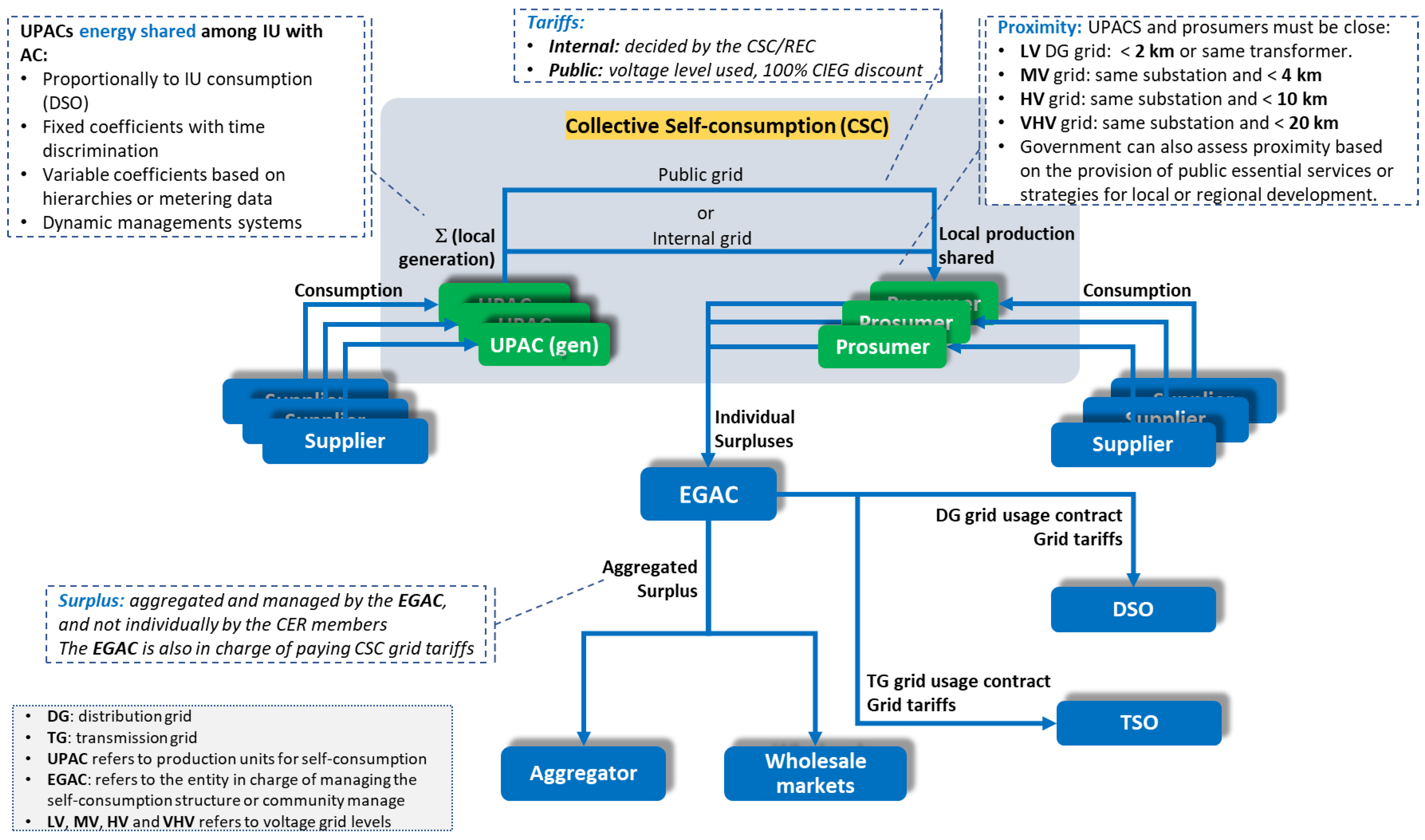
In most regulatory frameworks, in a CSC structure, prosumers who are geographically close (a concept that depends on how the EU directive is transposed to each EU member state) join to produce energy and share the surplus with the other CSC members. The sharing rules agreed by the CSC members determine the AC with which the DSO calculates, from the meter readings, (a) how much energy is supplied to each member by its supplier and how much is self-consumed from local production, and (b) for each community resource that is injecting energy, the amount to allocate among the consumers, thus defining the path followed by the energy. This path determines the access tariffs to be paid for the self-consumed energy [2]. Usually, no access tariffs are paid for the voltage levels of the supposedly unused grid. Additional subsidies may also apply, such as the partial or total exemption of the Cost of General Economic Interest (also called CIEG) in Portugal, that includes costs shared and paid by all end-consumers such as renewable generation subsidies, compensations for the transition to a competitive market, capacity payments or environmental policies. Figure 1 summarizes these concepts for the Portuguese self-consumption regulation, where UPACs refer to generation (production) units for self-consumption.

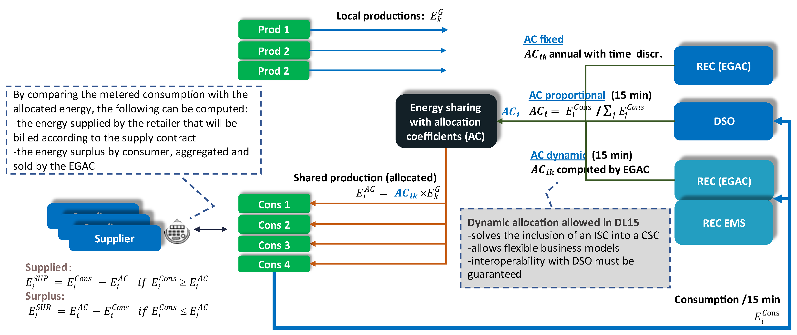
AC, see Figure 2, can be fixed, proportional to consumption, or dynamic and calculated by the REC itself, the latter (already in Decree Law 15/2022) being those that actually allow implementing business models adapted to the requirements of each REC [2]. Note also that the current law does not rule on the need of using only positive AC, but the Portuguese regulator ERSE is not likely to allow negative values when the new specific enforcement rules are developed. Note that negative AC may be understood as a way to increase competition at the retail market (see [2,17]).

The self-consumers participating in a CSC must communicate the internal governance rules to the DGEG (a Portuguese public administration body in charge of energy affairs) during the first 3 months of the UPAC. These governance rules must define, at least, the requirements for becoming a CSC member and to exit it; the deliberative majorities required; the methodology to share, for self-consumption, the energy produced locally and the correspondent tariffs’ payments; the destination of the energy surplus; and the commercial relationship policy and income sharing. UPAC licensing follows the same rules as for ISC.

The self-consumers of a CSC must appoint an EGAC (the entity in charge of managing the self-consumption), responsible for the CSC management procedures, including, among other things: the internal grid management; the link with the digital platform for the interactions with the public administration; the connection to the public grid and communication with the corresponding grid operators in terms of energy sharing and allocation coefficients; and the commercial relationship regarding the energy surplus, which can be sold directly to the wholesale market or through an Aggregator. If none of these options are taken, the energy surplus is otherwise delivered to the grid for free. In case of a REC or a CEC, the functions of the EGAC are performed by the communities themselves, or by another entity to which they delegate these functions. Finally, the self-consumers participating in a CSC, REC or CEC are jointly responsible for fulfilling the duties and obligations established by the current related regulation (DL15 and other applicable regulations).

2.2. Problem Description

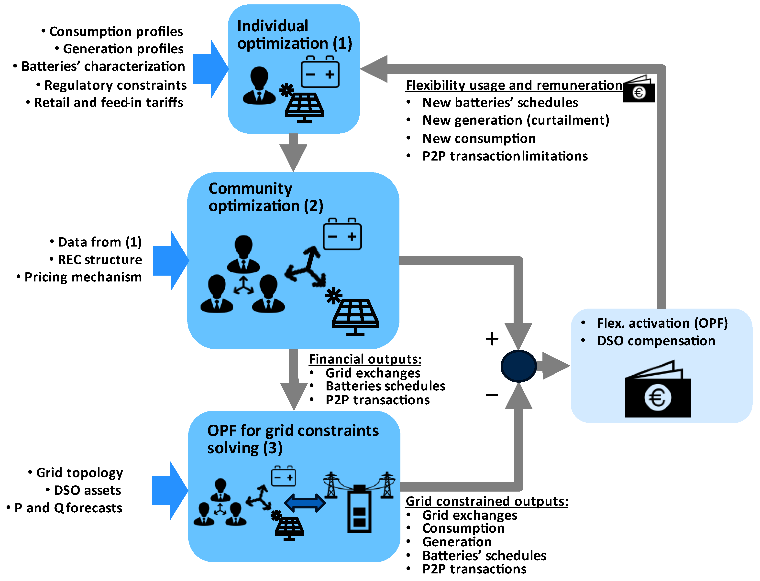
The problem addressed assumes that there is a microgrid with N prosumers that participate in a REC. In order to minimize the energy bills, increase prosumer engagement and guarantee the security of the operation of the local grid, a three-stage energy management methodology is proposed, as shown in Figure 3.

In the first stage, each prosumer, which can own a behind-the-meter battery and a generation unit, and can share local generation facilities with other prosumers, optimizes its battery schedule to minimize its energy bill considering its consumption, the total local generation and its supply and feed-in tariffs. Consumers must pay the local grid tariffs corresponding to the energy self-consumed, as is defined in the Portuguese regulation, since producers do not pay access tariffs.

In the second stage, the total REC’s energy bill is minimized, but guaranteeing that all prosumers face a new energy bill equal or less than the individual bill from stage one. This stage allows the community members to locally share their energy surplus to obtain an additional benefit for belonging to the REC without losing their individual benefits.

The third stage is an optimal power flow (OPF) performed by the operator of the local distribution grid, which could be the DSO or the REC itself in case the regulation allows the community to operate its own grid, to solve any existing grid constraints. To do so, the grid operator activates the flexibility needed at minimum cost, assuming that the existing flexibility is the re-schedule of the prosumers’ batteries, and in case this is not enough to solve the grid constraints, curtailment of the local generation or even the reduction of the prosumers’ consumption if needed.

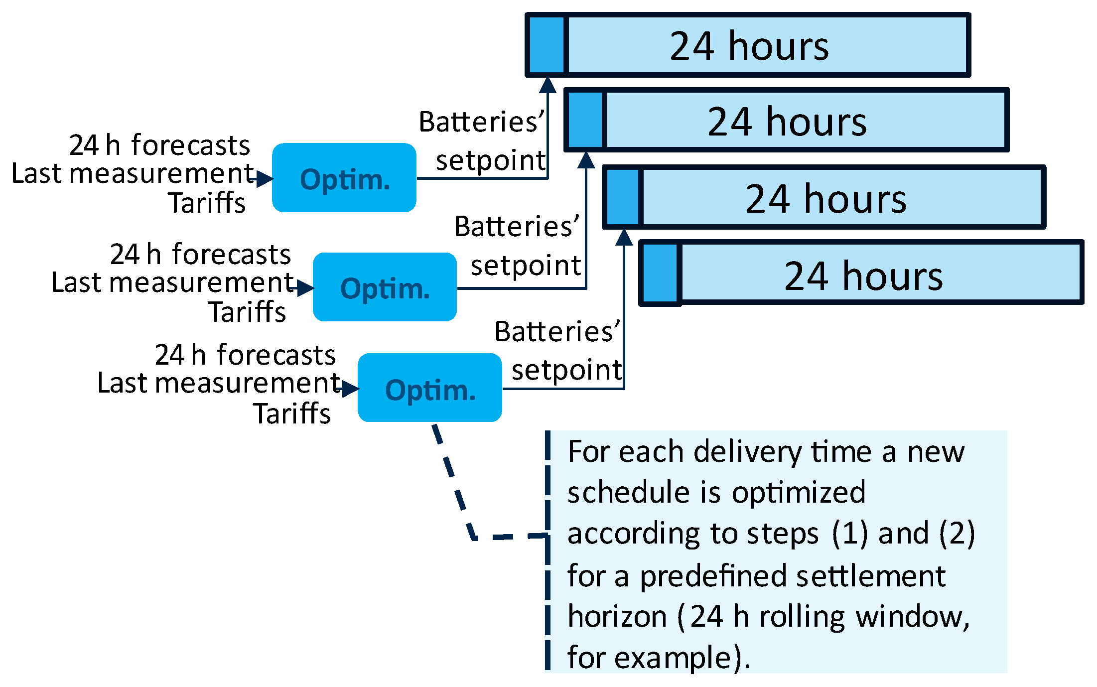
In case an automatic energy management system is considered, stages one and two can run for a rolling window of, for example, 24 h, to continuously recompute the optimal battery schedules and their set-point for the next delivery time. This procedure is shown in Figure 4. Note that a pricing mechanism (see [4,18]) must be decided for stage two to determine the financial compensations for the internal energy transactions, a decision which, as will be shown later, has strong implications on the behavior of the optimization performed in stage two.

Note, however, that these two steps can also be used to simulate the operation of a local energy market that could operate in the REC. In this case, the market environment itself would provide the market price (or prices in case of bilateral agreements) to be used for financial compensations of the internal transactions. However, each prosumer would need to forecast this local market price for each rolling window to be able to optimize its battery schedule.

3. The Three-Stage Model

3.1. Stage One: Individual Optimization

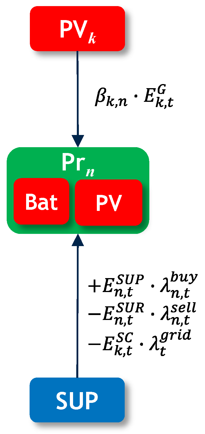
This stage corresponds to the individual optimization of the energy management of each prosumer n, and it is based on the energy exchanges of Figure 5. The prosumer has a behind-the-meter battery and a photovoltaic (PV) installation, and can also have a participation ${\beta }_{k,n}$ on an external generation facility k. Its energy imbalance is solved with its retailer that can either supply the energy deficit at price ${\lambda }_{n,t}^{buy}$ or buy its energy surplus at price ${\lambda }_{n,t}^{sell}$ (negative in Figure 5 to reflect an income).

Therefore, the following first stage optimization problem is proposed:

$$min{{\displaystyle \sum }}_{t\in T}\left(E_{n,t}^{SUP}·{\lambda }_{n,t}^{buy}-E_{n,t}^{SUR}·{\lambda }_{n,t}^{sell}+E_{n,t}^{SC}·{\lambda }_t^{grid}\right),$$

(1)

where the decision variables are the batteries’ charging and discharging schedules (see the problem constraints below), and where the objective function is the minimization of the total energy costs consisting of the cost of the energy bought from the supplier, the incomes for the energy sold back to the grid and the grid tariffs paid for the local external generation supply k. Note that ${\lambda }_{n,t}^{buy}$ and ${\lambda }_{n,t}^{sell}$ are final prices and must include the energy prices applied by the retailer but also the grid access tariffs and any other charge needed to compute these buying and selling prices. Since we are not considering resource sizing, capacity grid tariffs can be considered fixed and, therefore, do not need to be considered in the optimization problem. Note also that the third term of the objective function corresponds to the local grid tariffs that, at least in the Portuguese regulation, are applied to the energy $E_{n,t}^{SC}$ self-consumed by prosumer n, which is given by the following expression:

$$E_{n,t}^{SC}={{\displaystyle \sum }}_k\left(min\left(max\left(E_{n,t}^{CMET},0\right),{{\displaystyle \sum }}_k{\beta }_{k,n}·E_{k,t}^G\right)\right),$$

(2)

where $E_{n,t}^{CMET}$. is the net consumption measured at meter n (negative in case of generation, see Equation (4) below), which is used to compute the actual consumption (when $E_{n,t}^{CMET}$ is positive), and from it, the amount of self-consumed energy from the prosumer external facilities. It is assumed that supply and feed-in tariffs include the energy price and the correspondent grid access volumetric tariffs.

In addition, the following constraints must also be also considered:

$$E_{n,t}^{SUP}+{{\displaystyle \sum }}_k{\beta }_{k,n}·E_{k,t}^G=E_{n,t}^{CMET}+E_{n,t}^{SUR},$$

(3)

$$E_{n,t}^{CMET}=E_{n,t}^C+E_{n,t}^{BC}-E_{n,t}^G-E_{n,t}^{BD},$$

(4)

$$E_t^B=E_{t-1}^B+\left(E_{n,t}^{BC}·{\eta }^{BC}-\frac{E_{n,t}^{BD}}{{\eta }^{BD}}\right),$$

(5)

$$SO{C}^{min}\le SO{C}_{n,t}=\frac{E_{n,t}^B}{E_n^{BN}}\times 100\%\le SO{C}^{max},$$

(6)

$$\frac{E_{n,t}^{BC}}{\Delta t},\frac{E_{n,t}^{BD}}{\Delta t}\le P^{BMax},$$

(7)

$$E_{n,t}^{BC},E_{n,t}^{BD},E_{n,t}^B,E_{n,t}^{SUP},E_{n,t}^{SUR},SO{C}_{n,t}\ge 0,$$

(8)

where $E_{n,t}^{BC}$ and $E_{n,t}^{BD}$ are the charging and discharging schedules of the behind-the-meter battery (decision variables of this stage), $E_{n,t}^G$ is the prosumer consumption profile, $E_{n,t}^G$ its behind-the-meter generation profile, $E_{n,t}^B$ is the energy stored in the battery, $E_n^{BN}$ is its nominal capacity and $SO{C}_{n,t}$ its state of charge. Constraint (3) is the prosumer energy balance, (4) computes its net metered consumption, (5) computes the energy stored in the battery considering the charging and discharging efficiencies, with its input and output power limited by (7) and (6) computes and limits the battery’s state of charge (SOC). This stage provides the minimum energy bill $C_n^{ind}$ from (1) after the individual optimization of each prosumer n, which is an input for stage two.

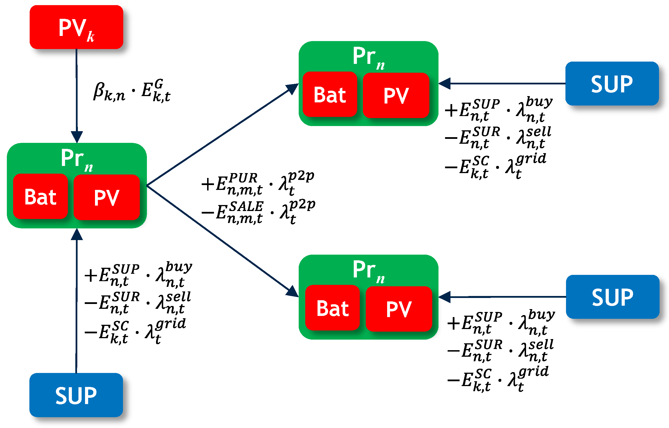
3.2. Stage Two: Collective Optimization

The second stage is a minimization of the collective REC bill using the existing flexibility, but also guaranteeing that the new individual energy bills of all peers are always equal to or less than their value $C_n^{ind}$ obtained in the individual optimization of stage one. Figure 6 represents the individual and community energy exchanges for a simplified example. Compared to Figure 5 (stage one), apart from the same energy exchanges of each prosumer with its retailer and with the facilities it partially owns, internal energy exchanges take place to share the local energy surplus among the community members, before injecting it back to the grid, so that a member n can sell its surplus $E_{n,m,t}^{SALE}$ to another member m, or locally buy an additional supply $E_{n,m,t}^{PUR}$.

In this case, the following optimization problem is proposed:

$$min{{\displaystyle \sum }}_{t\in T}\left({{\displaystyle \sum }}_{n\in N}\left(E_{n,t}^{SUP}·{\lambda }_{n,t}^{buy}-E_{n,t}^{SUR}·{\lambda }_{n,t}^{sell}+E_{n,t}^{SC}·{\lambda }_t^{grid}\right)\right),$$

(9)

where the decision variables are again the batteries’ schedules. The energy bill of the community is computed by aggregating all individual energy bills. Internal trades can be ignored since, at the community level, it is a zero-sum game, but internal supplies that used the local grid must pay the corresponding local grid tariff ${\lambda }_t^{grid}$, which are assumed to be paid by the consumers and not by the producers, as it is in the Portuguese regulation. In this case, the self-consumed energy is given by the following equation, where the locally allocated energy now includes the energy produced by the prosumer-owned facilities, but also net energy bought locally:

$$E_{n,t}^{SC}=min\left(max\left(E_{n,t}^{CMET},0\right),max\left({{\displaystyle \sum }}_m\left(E_{n,m,t}^{PUR}-E_{n,m,t}^{SALE}\right)+{{\displaystyle \sum }}_k{\beta }_{k,n}·E_{k,t}^G,0\right)\right).$$

(10)

The following constraint guarantees that sells equal purchases:

$$E_{n,m,t}^{PUR}=E_{m,n,t}^{SALE}.$$

(11)

In addition, constraint (3) from stage one needs to include internal sales and purchases, becoming:

$$E_{n,t}^{SUP}+{{\displaystyle \sum }}_k{\beta }_{k,n}·E_{k,t}^G+{{\displaystyle \sum }}_m\left(E_{n,m,t}^{PUR}-E_{n,m,t}^{SALE}\right)=E_{n,t}^{CMET}+E_{n,t}^{SUR}.$$

(12)

Note that constraints (4) to (8) from stage one still apply. Constraint (13) is added for each peer n to guarantee that it sees a benefit for participating in the community optimization, assuming a Pareto optimality where no peer can become worse off, so that its new energy bill, including the internal trades at price ${\lambda }_t^{p2p}$ (assuming a local uniform price) is always equal or less than the bill $C_n^{ind}$ obtained from the individual optimization

$${{\displaystyle \sum }}_t\left(E_{n,t}^{SUP}·{\lambda }_{n,t}^{buy}-E_{n,t}^{SUR}·{\lambda }_{n,t}^{sell}+E_{n,t}^{SC}·{\lambda }_t^{grid}+{{\displaystyle \sum }}_m\left(E_{n,m,t}^{PUR}-E_{n,m,t}^{SALE}\right)·{\lambda }_t^{p2p}\right)\le C_n^{ind}.$$

(13)

The formulated problem does not allow to unambiguously determine the internal financial exchanges between peers, but only the total amount sold or bought internally by each peer, so that an additional proportional criterion can be applied to determine them if needed.

Note also that this optimization problem will induce members with lower supply tariffs sell energy (supplied to them by their retailers) to other members with higher tariffs, even if they do not have an energy surplus, to minimize the REC energy cost. This leads to negative AC, as explained in [17]. Since regulation may not allow negative AC (see Section 2.1), this can be avoided by preventing members from selling more energy than what they own, so that the following constraint must be added:

$${{\displaystyle \sum }}_m\left(E_{n,m,t}^{SALE}-E_{n,m,t}^{PUR}\right)\le {{\displaystyle \sum }}_k{\beta }_{k,n}·E_{k,t}^G+max\left(-E_{n,t}^{CMET},0\right).$$

(14)

From this stage two, the final values of $E_{n,t}^{SUP},E_{n,t}^{SUR}\mathrm{and}{E}_{n,t}^C$ are used as inputs $(E_{n,t}^{SUP-s2}$, $E_{n,t}^{SUR-s2}\mathrm{and}{E}_{n,t}^{C-s2}$) in stage three to minimize the cost of the flexibilities activated, as described in the next section.

3.3. Stage Three: Flexibility Activation for Local Grid Constraint Solving

The third stage has the objective of guaranteeing that the local distribution grid constraints are not violated. To do so, as shown in Figure 3, an OPF is computed, where the decision variables are the batteries’ schedules, but also the consumption and generation of the individual prosumers and local generation facilities in case this is still needed. The objectives of this stage are:

• Guarantee that the grid constraints are not violated;
• Minimize the cost of the activated flexibility;
• Interfere minimally with the commercial energy exchanges (that are in fact settled as they result from stage two).

The flexibility activated is computed by comparing the batteries’ schedules and the consumption and generation profiles before and after running the OPF, that is, comparing stages two and three Its cost is computed as the cost increment of the prosumers due to the flexibility activation, including the utility loss entailed, which is assumed to be compensated by the DSO. Therefore, the objective function of this third stage is:

$$min{{\displaystyle \sum }}_{t\in T}\left({{\displaystyle \sum }}_n\left(\Delta E_{n,t}^{SUP}·{\lambda }_{n,t}^{buy}-\Delta E_{n,t}^{SUR}·{\lambda }_{n,t}^{sell}-\Delta E_{n,t}^C·{\lambda }_{n,t}^{buy}·\tau +\Delta E_{n,t}^{SC}·{\lambda }_t^{grid}\right)\right).$$

(15)

As can be seen, the cost of the objective function is computed as the impact the flexibility activation has on the prosumers’ costs as a result of a modification on the energy exchanges with their prosumers given by $\Delta E_{n,t}^{SUP},\Delta E_{n,t}^{SUR}$, and on the prosumers utility due to the variation $\Delta E_{n,t}^C$ of their consumption, which has been valued at the retailer supply price ${\lambda }_{n,t}^{buy}$ they are willing to pay. We further include a multiplication factor $\tau$ to prioritize other forms of flexibility overload curtailment and aid on the solvers’ convergence. Constraints (5) to (8) must be added to model the battery behavior, and constraints (11) and (12) to compute the energy supplied and surplus after activating flexibility. In addition, the following constraints must be included:

$$\begin{gathered} E_{n,t}^{SUP}=E_{n,t}^{SUP-s2}+\Delta E_{n,t}^{SUP} \mathrm{and} E_{n,t}^{SUR}=E_{n,t}^{SUR-s2}+\Delta E_{n,t}^{SUR}, \\ {E}_{n,t}^C=E_{n,t}^{C-s2}+\Delta E_{n,t}^C \Delta E_{n,t}^C \le 0, \end{gathered}$$

(16)

$${{\displaystyle \sum }}_k{E}_{k,t}^G-{{\displaystyle \sum }}_n\left(E_{n,t}^{CMET}\right)+E_{ij,t}=0, j\in Br\left(i\right), n,k\in Met\left(i\right)),$$

(17)

$${\displaystyle \sum }_{k}R{E}_{k,t}^G+{\displaystyle \sum }_n\left(R{E}_{n,t}^{BD}+R{E}_{n,t}^G-R{E}_{n,t}^{BC}-R{E}_{n,t}^C\right)+R{E}_{ij,t}=0, j\in Br\left(i\right), n,k\in Met\left(i\right),$$

(18)

$$Q_{k,t}^{cb}\in \left\{Q_{k,t}^{cb}\right\},\forall k\in N_{cb} \mathrm{and} Ta{p}_{k,t}\in \left\{Ta{p}_{k,t}\right\},\forall k\in N_{OLTC},$$

(19)

$${\Phi }_{t,ref}=0,$$

(20)

$$V_{i.t}^{min}\le \left|V_{i,t}\right|\le V_{i.t}^{max} \mathrm{and} {\left|S_{ij,t}\right|}^2\le {\left(S_{ij}^{max}\right)}^2, \forall ij\in Br$$

(21)

$$P_{i,t}=\left|V_{i,t}\right|{{\displaystyle \sum }}_{j\in Br\left(i\right)}\left[\left|V_{j,t}\right|\left(G_{ij}\ast cos{\theta }_{ij,t}+B_{ij}\ast sin{\theta }_{ijt}\right)\right],$$

(22)

$$Q_{i,t}=\left|V_{i,t}\right|{{\displaystyle \sum }}_{j\in Br\left(i\right)}\left[\left|V_{j,t}\right|\left(G_{ij}\ast sin{\theta }_{ij,t}-B_{ij}\ast cos{\theta }_{ij,t}\right)\right].$$

(23)

The decision variables are again the batteries’ schedules, $E_{n,t}^{BC}$ and $E_{n,t}^{BD}$, but also the locally generated energy $E_{k,t}^G$ that can be curtailed ($\Delta E_{k,t}^G\le 0$), and the peers’ net consumption, $E_{n,t}^{CMET}$, so that their injection to the grid can also be curtailed or their consumption reduced. Including the utility loss of the prosumers is needed in (15) to avoid curtailing all energy consumption to minimize the energy bill. In fact, to prioritize other flexibilities over a consumption reduction, which entails a loss of comfort, the prosumer utility in (15) can be valued at a cost slightly larger than ${\lambda }_{n,t}^{buy}$ (controlled by the $\tau$ multiplication factor).

Constraint (16) relates the new values of the variables $E_{n,t}^{SUP}$, $E_{n,t}^{SUR},E_{n,t}^C,E_{k,t}^G$ and $E_{n,t}^G$ with their values at stage two (denoted by s2) allowing to assess their difference between stages two and three.

Constraints (17) to (23) are the typical OPF constraints. Constraints (17) and (18) are the active and reactive energy balances at bus $i$ being $E_{ij,t}$ the exiting energy through branch $ij$, with $j\in Br\left(i\right)$ the set of buses $j$ connected through a branch $ij$ to bus $i$, and $n\in Met\left(i\right)$ the set of all meters connected to bus $i$.

Constraint (19) models the discrete step positions of the capacitor banks and on-load tap changers (OLTC) of the grid operator, $N_{cb}$ and $N_{OLTC}$ being the number of capacitor banks and OLTCs, respectively.

Constraint (20) sets the voltage angle at the reference bus and, (21) limits the voltage magnitude of all buses $i$ and the direct and inverse $ij$ branches’ flow to their thermal limit, being $Br$ the set of all grid branches.

Constraints (22) and (23) are the active and reactive powers at bus $i$ considering all branches $ij$ connected to node $i$, being $V_{j,t}$ the voltage at the other node of branch $ij$, $G_{ij}$ and $B_{ij}$ the real and imaginary parts of the admittance of branch $ij$, and ${\theta }_{ij,t}$ the difference in voltage angle between bus $i$ and bus $j$ the line $ij$ is connected to.

3.4. Settlement

The settlement of each prosumer with its retailer is usually based on the computation of the energy allocation coefficients, as it is the case of France [19], Spain [20] and Portugal [21] (see also [2]). These coefficients allow the DSO to compute, from the smart meters’ readings, how much energy is supplied by the retailers to their customers, how much is self-consumed from local production, and for each REC resource injecting energy, the amount allocated to the resource consumption, thus defining the path followed by the energy [2]. This path can then be used to determine the access tariffs to be paid by the self-consumed energy, where it is a common strategy to pay only for the grid voltage levels used. In case dynamic allocation coefficients are in place, the REC manager can compute the allocation coefficients for each settlement period according to its own rules, which allows to reflect the real internal energy sharing. Otherwise, the most efficient type of coefficient should be selected (those that share the internal surplus proportionally to the consumption in the case of the Portuguese regulation, since they minimize the total community energy surplus), but additional internal compensations are needed to approximate the final settlement to the ideal one.

Assuming dynamic coefficients, already considered in the Portuguese regulatory framework [3], still to be operationalized by the Portuguese regulator ERSE, and assuming, for simplicity, that all resources are connected at the same voltage level and that energy is allocated from a pool of all energy injected to the grid by the community members and generation resources, then the allocation coefficients corresponding to the stage two proposed can be computed as:

$${\alpha }_{n,t}=\frac{{{\displaystyle \sum }}_k{\beta }_{k,n}·E_{k,t}^G+max\left(-E_{n,t}^{CMET},0\right)+{{\displaystyle \sum }}_m\left(E_{n,m,t}^{PUR}-E_{n,m,t}^{SALE}\right)}{{{\displaystyle \sum }}_n\left({\beta }_{k,n}·E_{k,t}^G+max\left(-E_{n,t}^{CMET},0\right)\right)}.$$

(24)

Indeed, the energy allocated to a REC member is the energy locally produced and owned by itself plus the net local surplus bought, divided by the total local net energy produced.

When the peers sell more energy than they own, arbitrage with retailers’ tariffs takes place among peers, providing more competition at the retail level, which can lead to negative AC as was already explained. Since regulation will probably not yet allow negative AC, constraint (14) can be added to stage two to guarantee positive AC. Both cases will be studied in the results section.

In case a member is still consuming after the energy allocation, it will have the following obligation to pay (OP) to its retailer:

$$O{P}_{n,t}^{SUP}=max\left(E_{n,t}^{CMET}-{{\displaystyle \sum }}_k{\beta }_{k,n}·E_{k,t}^G-{{\displaystyle \sum }}_m\left(E_{n,m,t}^{PUR}-E_{n,m,t}^{SALE}\right),0\right)·{\lambda }_{n,t}^{buy}.$$

(25)

In case there is a local generation surplus not totally allocated to the members who are consuming, then, according to the Portuguese regulation, the REC manager (EGAC in the Portuguese terminology) aggregates this net surplus to sell back to the market or to a facilitator at a regulated feed-in tariff. For those peers with net production ($E_{n,t}^{CMET}\le {{\displaystyle \sum }}_k{\beta }_{k,n}·E_{k,t}^G+{{\displaystyle \sum }}_m\left(E_{n,m,t}^{PUR}-E_{n,m,t}^{SALE}\right)$), assuming a unique selling price ${\lambda }_{EGAC,t}^{sell}$, they acquire a collection right (CR) given by:

$$C{R}_{n,t}^{SUR}=max\left({{\displaystyle \sum }}_k{\beta }_{k,n}·E_{k,t}^G+{{\displaystyle \sum }}_m\left(E_{n,m,t}^{PUR}-E_{n,m,t}^{SALE}\right)-E_{n,t}^{CMET},0\right)·{\lambda }_{EGAC,t}^{sell}.$$

(26)

The internal settlement leads to the following obligation to pay and CR for each settlement period and member n:

$$\begin{gathered} O{P}_{n,t}^{p2p}={\displaystyle \sum }_m^{N}max\left(E_{n,m,t}^{PUR}-E_{n,m,t}^{SALE},0\right)·{\lambda }_t^{p2p} \\ C{R}_{n,t}^{p2p}={\displaystyle \sum }_m^{N}max\left(E_{n,m,t}^{SALE}-E_{n,m,t}^{PUR},0\right)·{\lambda }_t^{p2p} \end{gathered}$$

(27)

In case stage three needs to activate flexibility, then the final consumption of each member can lead to a different settlement with its retailer which needs to be compensated by the DSO. Then, each member acquires a CR for the provision of flexibility given by:

$$C{R}_{n,t}^{flex}=\Delta E_{n,t}^{SUP}·{\lambda }_{n,t}^{buy}-\Delta E_{n,t}^{SUR}+\Delta E_{n,t}^C·{\lambda }_{n,t}^{buy}+\Delta E_{n,t}^{SC}·{\lambda }_t^{grid}.$$

(28)

4. Case Studies and Results Analysis

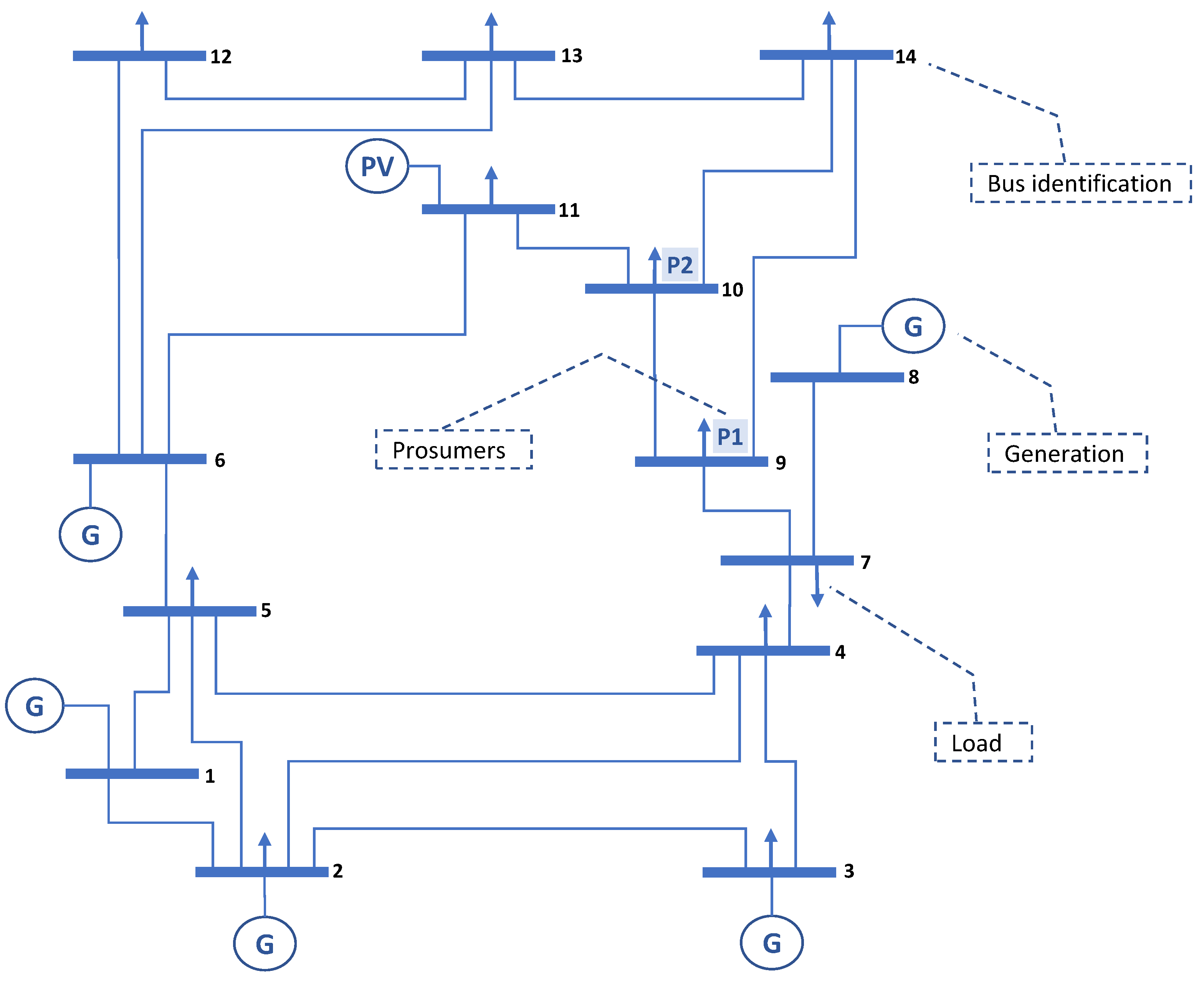
To validate the proposed methodology, the IEEE 14 bus test case of Figure 7 [22] was used; although stages one and two do not include grid constraints, stage three does. This test system was chosen for two main reasons: (1) It considers buses in low- and medium-voltages, which allows an evaluation of the impact of forming a residential community on both grids; (2) It is a relatively simple test system, rich enough for the test to be performed but allowing an easier interpretation of the results than more complex grids. The community has two prosumers, P1 and P2, with load, battery and PV generation all behind-the-meter, located at buses nine and ten, respectively, and an external PV generation equally shared (50%) by both prosumers and located at bus 11, as shown in Figure 7.

Load and solar PV generation profiles were both taken from [23], where they are publicly available, and could be made available by the authors by email. The batteries’ capacity was set to 1 kW and its charging and discharging power to 0.25 kW, with the same charging and discharging efficiencies of 90%, and minimum and maximum SOC of 10% and 90%, respectively. It was also assumed that their initial and final SOC for every scenario was 50%. For scenario V and beyond, where stage three is considered, the reference bus can absorb the energy surplus or inject the energy deficit from the main network. Buses one and two work as PQ buses with their lower and upper voltage limits set, at maximum, between 0.9 and 1.1, respectively. To trigger grid issues, the influence of prosumer’s power flows on the grid constraints was amplified by a factor of 1000. This was needed to test the stage three of the proposed methodology, considering that the peers’ resources and energy patterns were set according to sensible criteria, and considering the robustness of the grid selected, but without compromising the generality of the proposed approach.

The supply access tariffs correspond to the most frequent low voltage Portuguese tariff for end consumers for year 2018. The economic assessment did not take into consideration the fixed (power) term of the access tariff, nor the value added tax (VAT) nor any other concept that may be added to the access tariff.

Finally,

Table 1. Buying and selling retailers’ prices for each prosumer, in EUR/kWh.

Prosumer	${\mathit{\lambda }}_{\mathit{n},\mathit{t}}^{\mathit{b}\mathit{u}\mathit{y}}$	${\mathit{\lambda }}_{\mathit{n},\mathit{t}}^{\mathit{s}\mathit{e}\mathit{l}\mathit{l}}$
P1	0.20	0.02
P2	0.18	0.04

presents the prosumers’ buying and selling prices from their retailers, where no time discrimination was considered.

All simulations were performed for a 24-h horizon with hourly resolution.

Stage three OPF was implemented with a simplified linearized version based on the computation of the grid sensitivity indices [24], already used for example in [25] for flexibility needs’ computation and activation.

The algorithms were implemented in Python, using the modeling language Pyomo [26] and the open-source COIN-OR Branch-and-Cut MILP solver [27] and conducted on a Laptop PC with AMD^® Ryzen^® CPU 5 PRO [email protected] GHz and a 16 GB RAM.

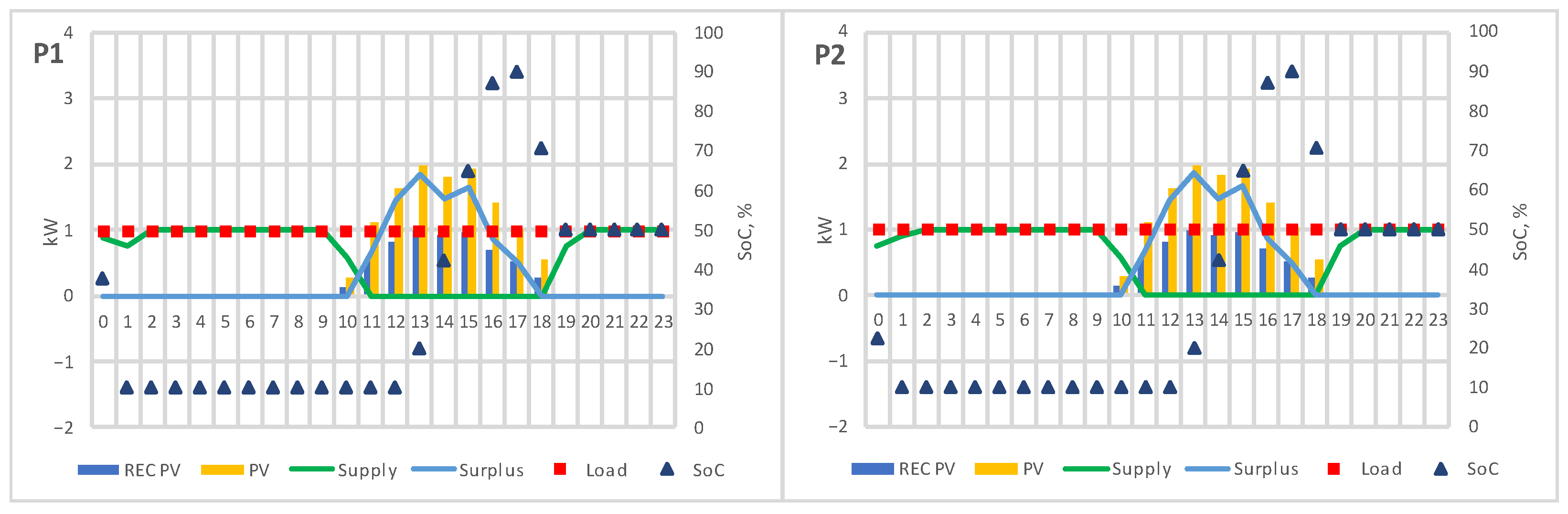
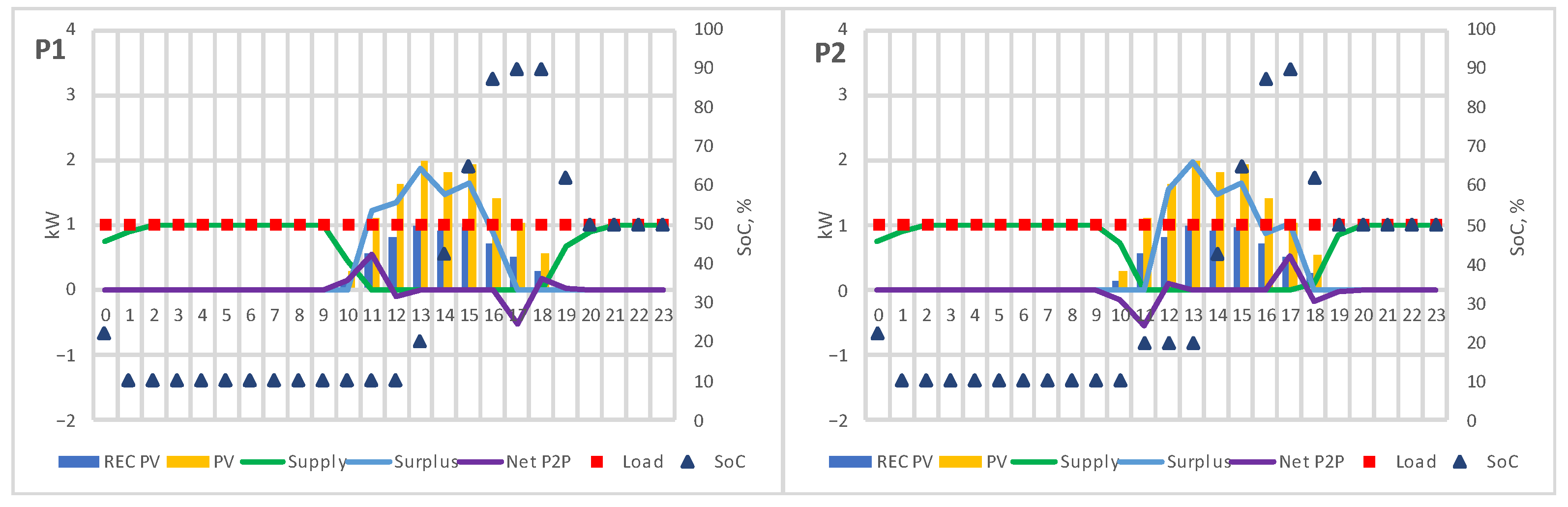
4.1. Scenario I

Figure 8 shows the results of stage one with the communities’ solar PV generation (REC PV shared by the prosumers), and, for each prosumer, its solar PV generation, the energy supplied by the retailer, the energy surplus sold to the retailer, its load profile and the SOC of its battery.

As can be seen, both prosumers resort to the battery in the first periods to avoid buying energy from the suppliers. Then, there is a constant supply from the suppliers until the PV generation becomes positive. At this point, the supply from the suppliers goes to 0, the batteries charge and there is also a surplus sold back to the retailers. Note that, since there is no time discrimination among retailer prices, provided the batteries reach their maximum SOC (90%), the share between charging and selling back is undetermined. Finally, when the PV generation is no longer available batteries are discharged again to comply with the 50% SOC constraint at the end of the day.

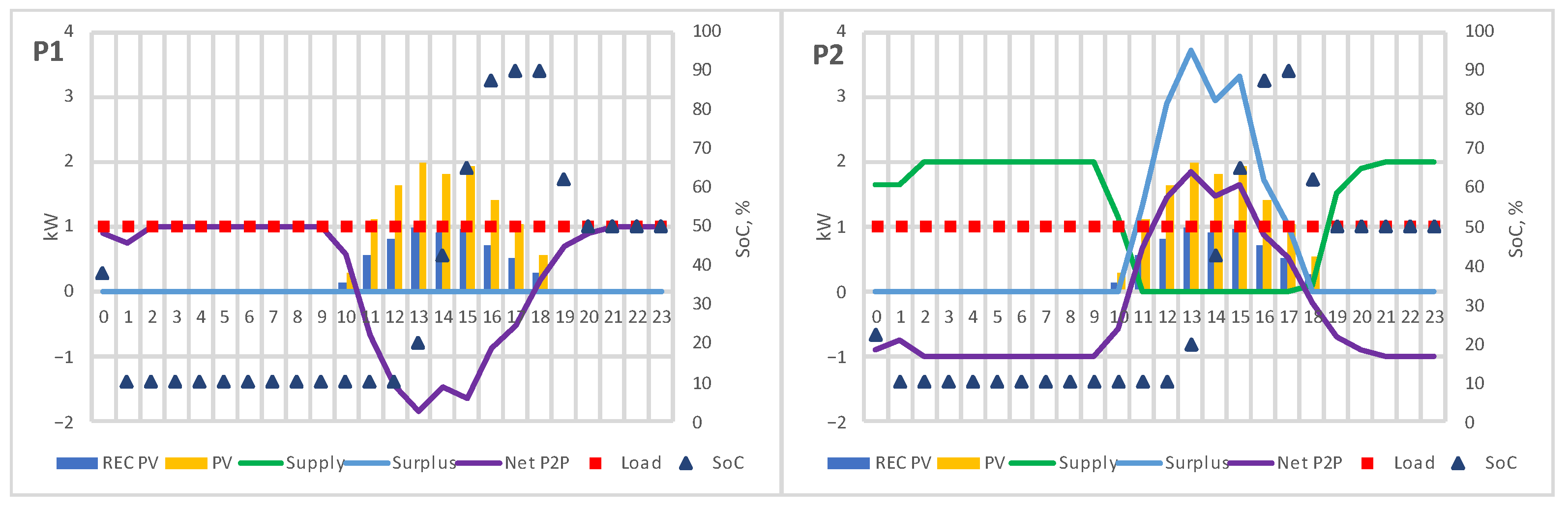
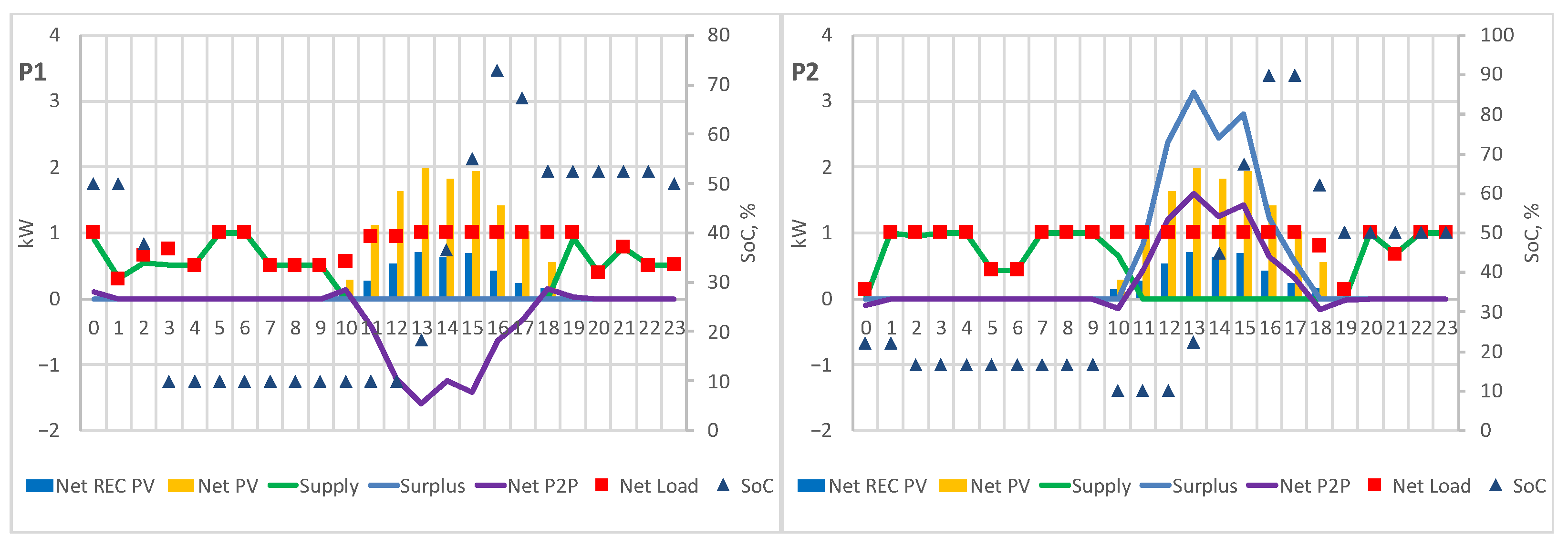
Figure 9 shows the results from stage two, including the net P2P for each agent, when constraint (13) is not considered, i.e., the individual benefits of stage one do not need to be preserved in stage two. Please note that “Supply” is always 0 and is overlapped by “Surplus” in the left figure.

As can be seen, when there is no solar PV generation, P2, with lower supply prices (${\lambda }_{1,t}^{buy}>{\lambda }_{2,t}^{buy}$), buys the energy deficit of both prosumers (green line) and sells part to P1 through P2P (purple line). Conversely, when there is solar PV production, P1 charges its battery and sells its surplus to P2 through P2P that sells it back to its retailer, since he profits from a larger selling price (${\lambda }_{2,t}^{sell}>{\lambda }_{1,t}^{sell}$). Note that this behavior, allowing for all peers to profit from the best peer tariffs among all members, is only possible when negative AC are allowed, i.e., when constraint (14) is not considered.

To analyze the impact of the internal transaction price on the total costs of the prosumers, an economic assessment was performed under different price scenarios: (a) the MMR described in [18] and computed here as the average between the lowest selling price to the retailer and the highest buying price from the retailer (0.11 EUR/kWh), (b) a price between the MMR and the lowest selling prices (0.03 EUR/kWh) and (c) a price between the two highest buying prices (0.19 EUR/kWh). The results are compared to the individual optimization (IND) of stage one, where no P2P transactions take place. To properly address this analysis, constraint (13) was deactivated.

Table 2. Prosumer’s total costs in EUR for the individual optimization (IND) and three internal prices under Scenario I constraints.

	IND	(a) 0.11 EUR/kWh	(b) 0.03 EUR/kWh	(c) 0.19 EUR/kWh
Prosumer 1	2.83	0.96	0.44	1.48
Prosumer 2	2.36	4.00	4.52	3.48

presents the total costs for each prosumer through different internal prices and from the individual optimization, in EUR.

Comparing the results between the collective and individual optimizations, it is possible to see that the fairer internal price is 0.19 EUR/kWh. This is because P2 is, in fact, paying most of the supply to the REC peers, due to its lower tariffs, which is better compensated by setting the internal price at 0.19 EUR/kWh, closer to its buying price. A relevant conclusion is that the internal price is key for a fair share of the collective benefits when the REC profits from the better peer tariffs to supply other members. Nonetheless, even if an internal compensation is performed, as in scenario I-case (c) with a price closer to P2 buying price, P2’s net cost is still harmed by the internal transactions even if the REC obtains a larger global profit. Alternatively, unless being a less efficient solution for the REC, constraint (13) can be considered in stage two as shown next.

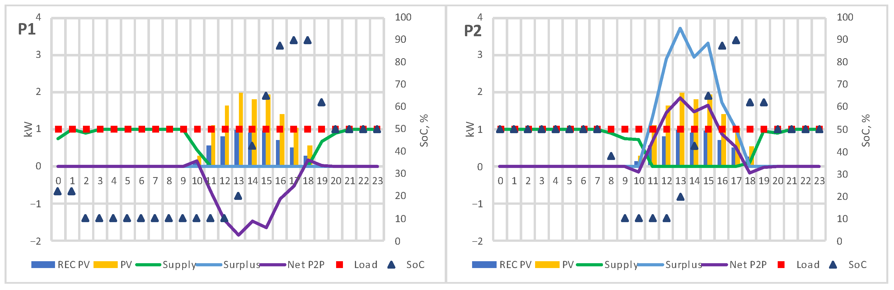
4.2. Scenario II

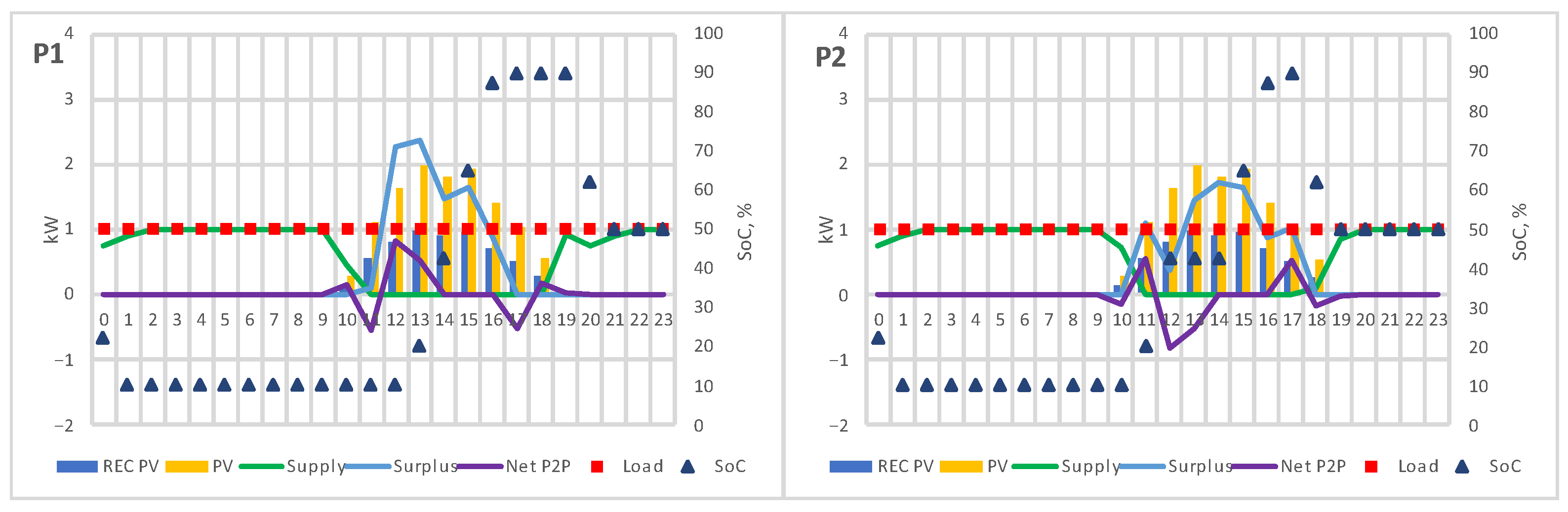
This scenario is similar to stage two of scenario I but instead considers constraint (13) to prevent prosumers’ total costs from exceeding those from their individual optimizations. The results are visually depicted in Figure 10.

Since both prosumers have the same demand and generation profiles, and since their new energy cost must be equal to or lower than the cost from the individual optimization (Figure 9), P2P (purple line) is significantly reduced with respect to the previous scenario when compared to Figure 9, to avoid harming P2’s net cost. Indeed, when the internal price is computed as the MMR, in this scenario, P2’s net cost after stage two remains the same as in stage I (EUR 2.36). Although the net cost for P1 increases in relation to Scenario I, it remains at EUR 2.83 (same as in stage I) since the cost increment is only 0.05% (which translates into less than EUR 0.01). The cost for the whole community also increases in relation to Scenario I, from EUR 4.96 to EUR 5.19, or approximately 5%.

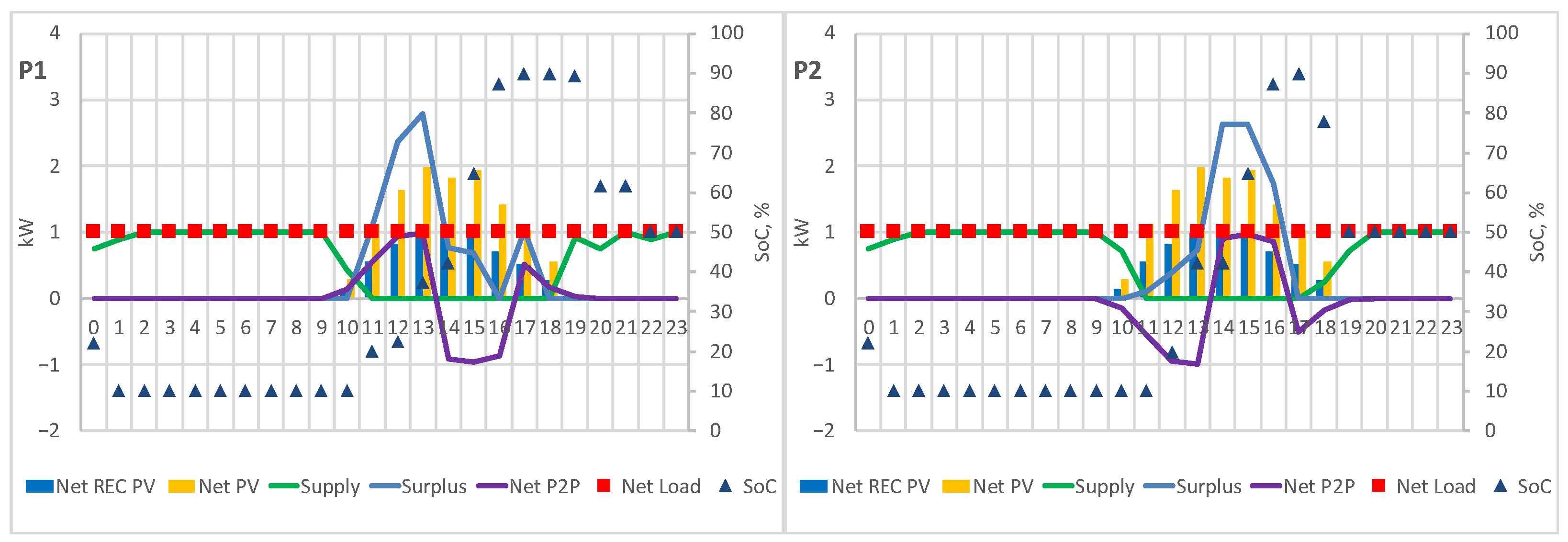
4.3. Scenario III

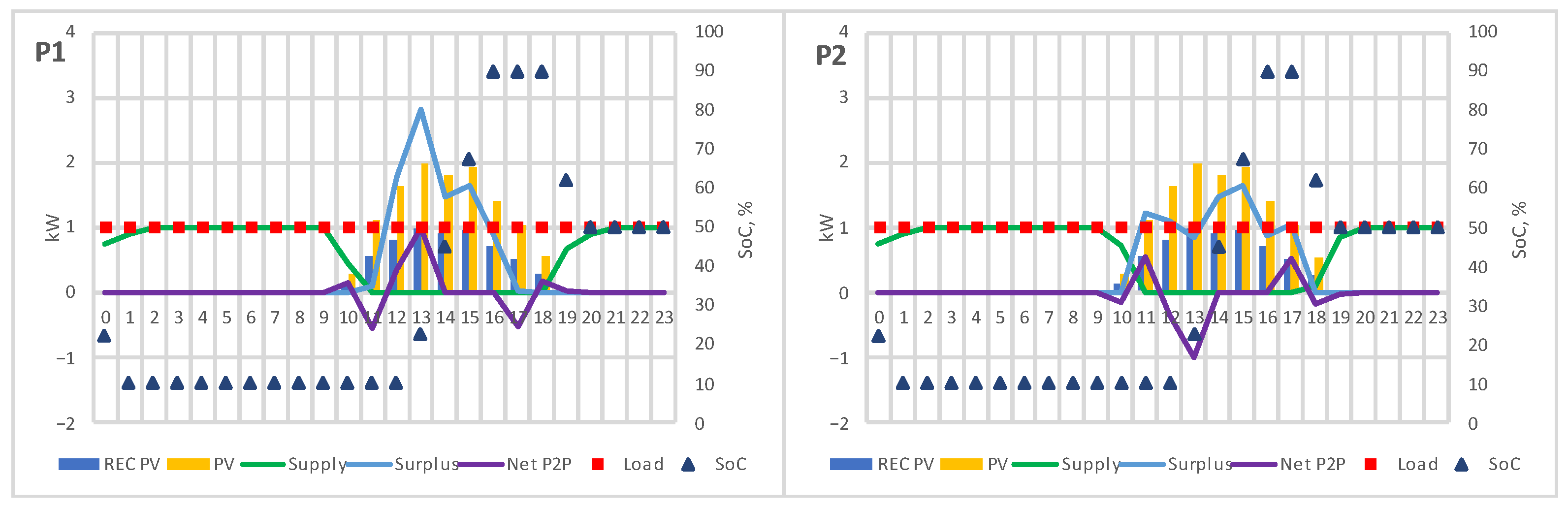
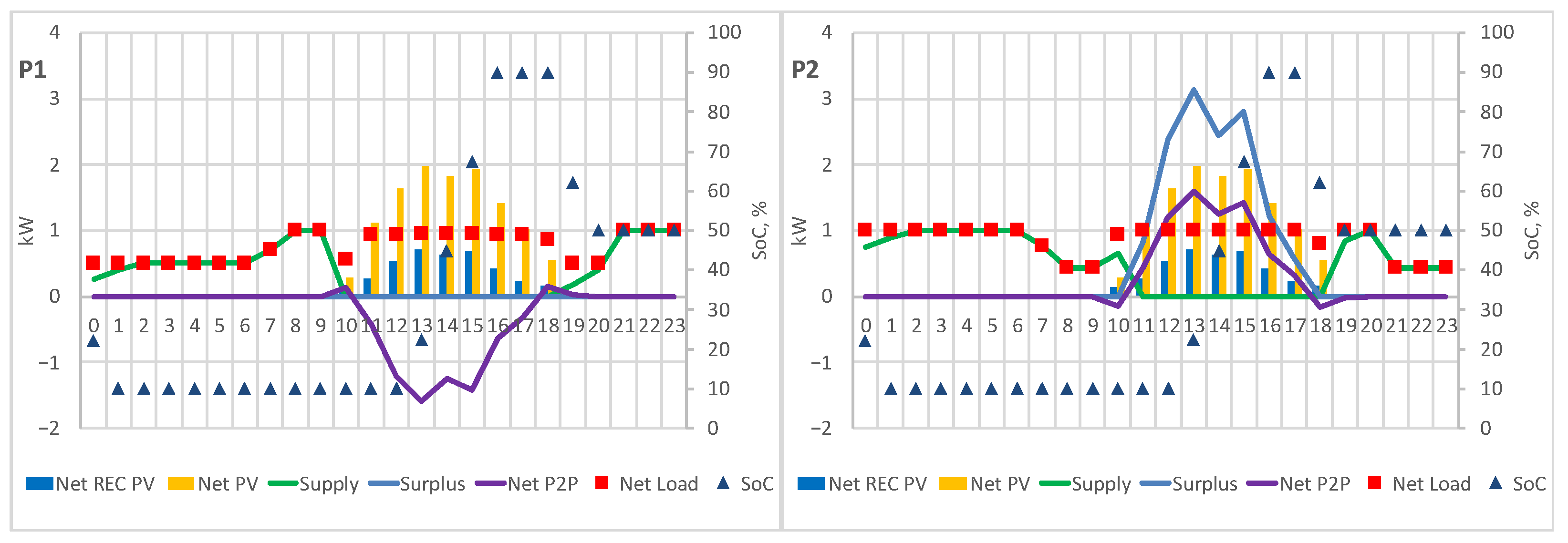
Figure 11 is as scenario II but forcing positive AC.

As can be observed, positive AC led to results very similar to those obtained with negative AC when constraint (13) is included. Indeed, constraint (13) significantly limits the P2P exchanges to protect P2’s net cost, so that less of P1’s supply comes from P2. Since AC limits to 0 the supply from P2 to P1 due to its lower prices when P2 has no local generation, both cases are very similar, with no differences observed in the costs of both prosumers.

4.4. Scenario IV

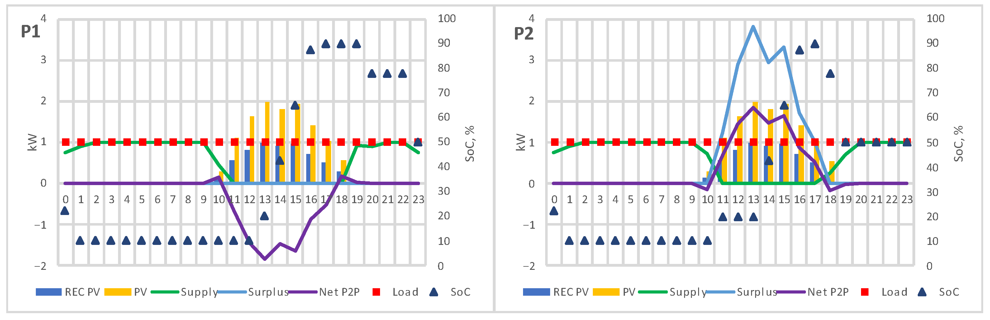
Figure 12 depicts a scenario similar to scenario III with positive AC and without constraint (13).

It is interesting to remark that, firstly, the volume of P2P exchanges is larger than in scenario III, since constraint (13) significantly limits these exchanges to avoid harming the net cost of REC peers with better tariffs, and secondly, that even if the volume of P2P exchanges is larger in this scenario, almost no supply of P1 comes from P2. Indeed, P2 cannot share with P1 more energy than it generates locally, since it is not possible with positive AC. However, at hours 10 and 18, when the solar generation is already present, P2 can share its local generation with P1, consuming more from its retailer, reducing the REC total bill. Numerically, the REC cost after stage two is EUR 5.02, resulting from a cost of EUR 2.04 for P1 and EUR 2.98 for P2. Compared to Scenario I (with the MMR as internal price), where negative AC were permitted, the cost of the community increases by 1.2%. The cost of P2 also increases in relation to its individual (or stage I) cost but is smaller than the one obtained at Scenario I, which highlights the importance that negative AC were having for reducing costs.

This also means that the internal P2P price is key for a fairer sharing of the collective benefits. Indeed, when constraint (13) is active, P2P exchanges take place only if they do not aggravate the net cost of any prosumer. Figure 13 depicts a similar case to the one analyzed in scenario II but with an internal price of 0.19 EUR/kWh, while in Figure 14 the internal price is 0.03 EUR/kWh, both with constraint (13) active. Results can be consulted at

Table 3. Prosumer’s total costs in EUR for the individual optimization (IND), considering different internal prices, with positive AC enforcement and with stage 1 compliance constraint.

	IND	(a) 0.19 EUR/kWh	(b) 0.03 EUR/kWh
Prosumer 1	2.83	2.82	2.70
Prosumer 2	2.36	2.36	2.32

.

As can be seen, in this case, with positive AC, a fairer internal price is a lower one that allows a better compensation of the peers involved (P1 benefit goes from 0.35% to 4.6% and P2 benefit from 0% to 1.7%), leading to a larger volume of P2P exchanges, so that the community profits better from the local energy for self-consumption. Indeed, as can be seen in Figure 14, P2P transactions are very similar to those of Figure 12, where constraint (13) is not active.

4.5. Scenario V (Stage 3)

In this scenario, the grid of Figure 7 is now considered to test stage three. Running a power flow using stage two results, highlights possible overvoltage problems in nodes six to twelve. However, when setting the voltage limits to $0.9\le V_{i,t}\le 1.1\left(\mathrm{p}.\mathrm{u}.\right)$ as defined in IEEE P1547 norm [28], the maximum voltage reached is 1.09 p.u. at bus seven, so no flexibility activation is needed.

Indeed, the application of stage three leads to a null flexibility cost, which is the value of the objective function (15) of stage three (with $\tau$ set to 1.3), and no differences should appear among stage two and three for a determined problem. However, the use of constant retail tariffs leads to a non-determined problem with multiple solutions with the same cost as that of stage two. This is why Figure 15 shows small differences from stage two of Scenario III (Figure 11). 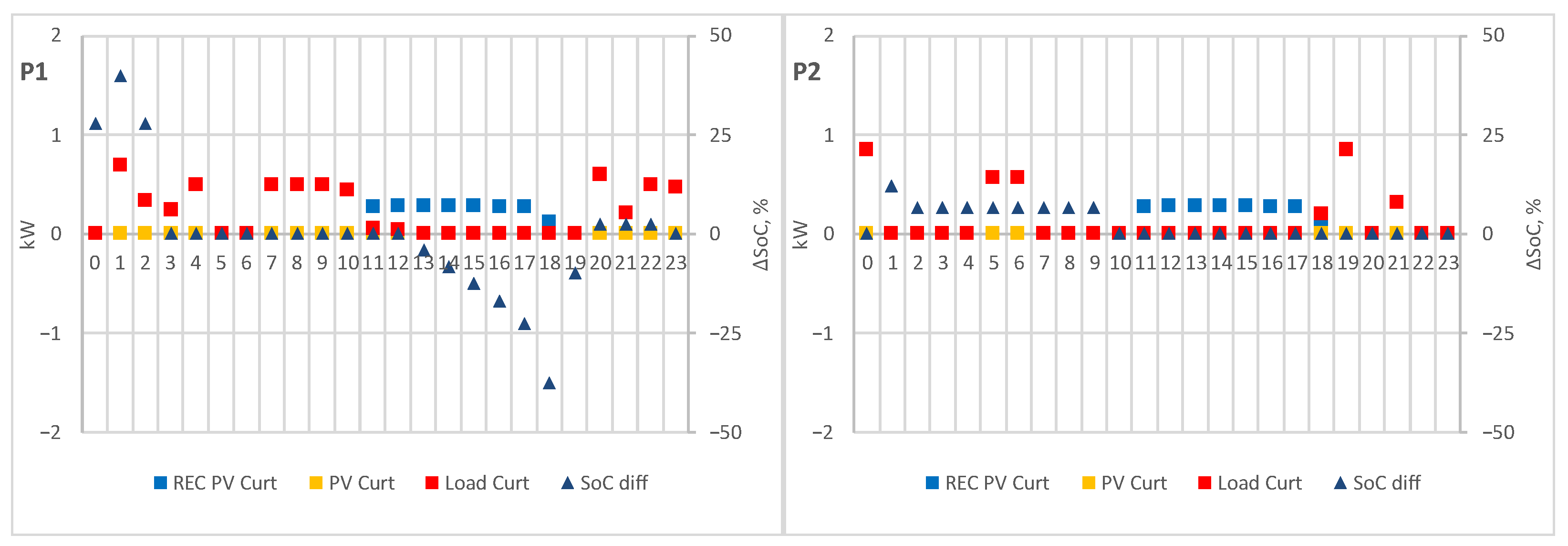This is also why Figure 16 does not show any load curtailment, but rather a difference from scenario III battery dispatch which does not correspond to a flexibility activation. 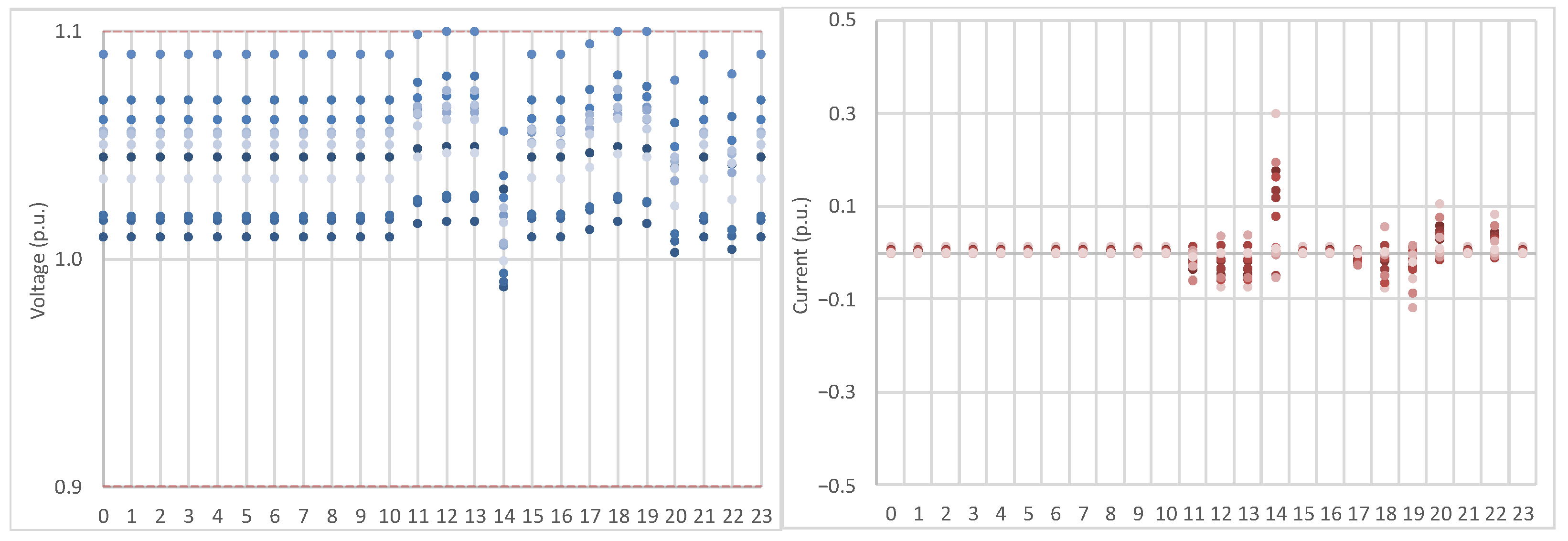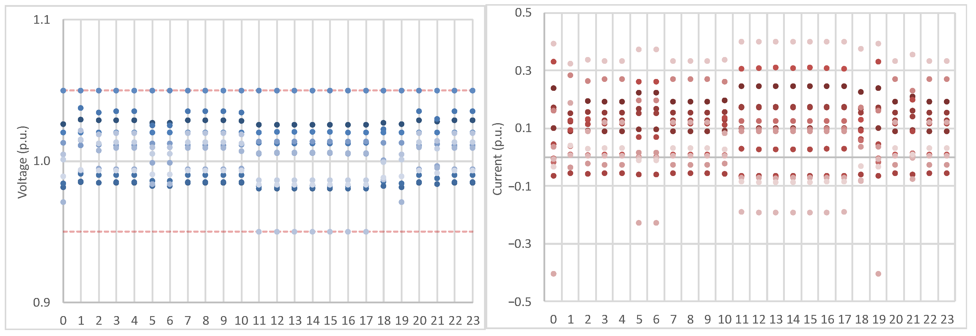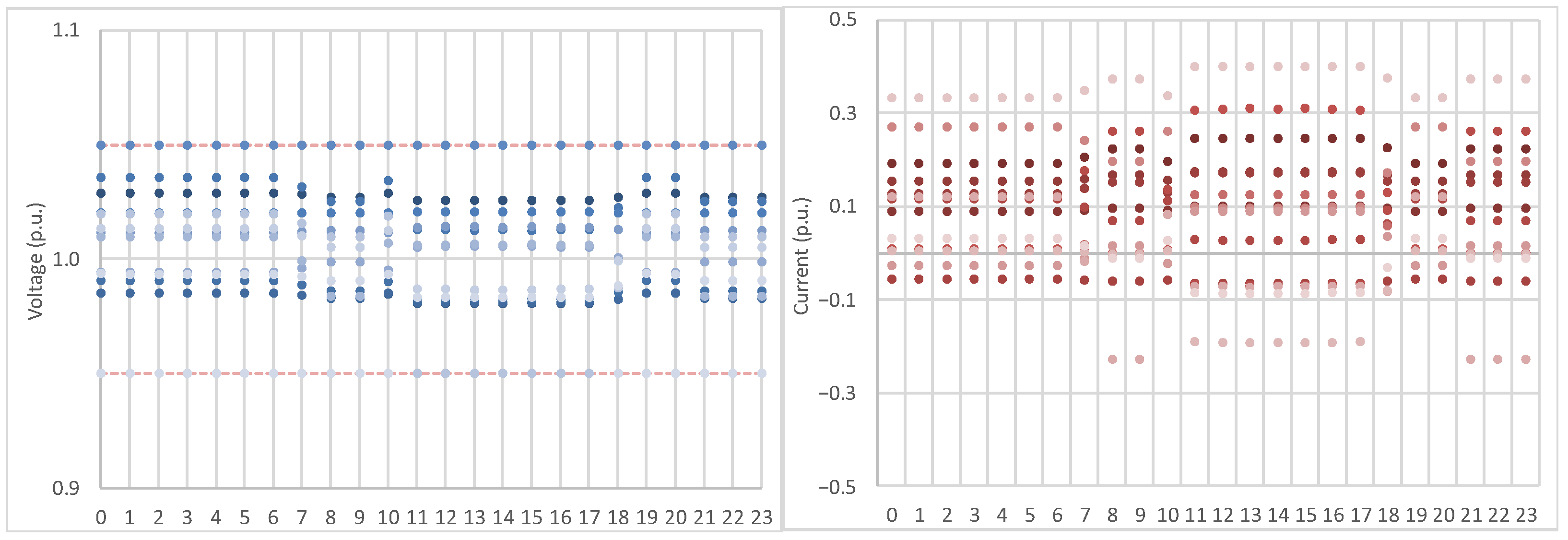Figure 17 depicts the voltage of the 13 buses and the currents in the 14 branches of the grid for each time-step of the simulated horizon. As can be seen, all voltages and currents are within their normal operation limits.

We also found that, with $\tau <1.3$, undesired load curtailments may appear that lead to negative flexibility costs. This is an indication that, without properly valuing the loss of comfort, the algorithm may encounter opportunities to leverage that source of flexibility through an undesired behavior.

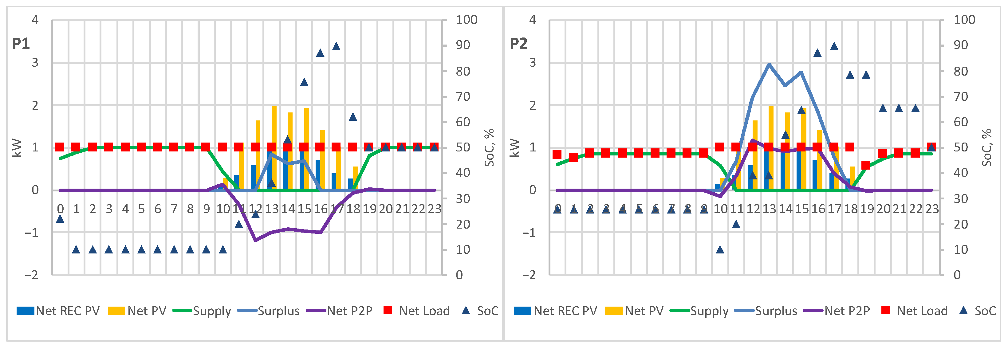
4.6. Scenario VI (Stage Three)

When reducing the voltage limits to $0.92\le V_{i,t}\le 1.08\left(\mathrm{p}.\mathrm{u}.\right)$ stage three activates load curtailment at P2 (2.4 kWh or 10% of total load) and generation curtailment at the community generation (1.1 kWh or 9.3% of total external PV generation), with a resulting flexibility cost for the community of EUR 0.05 (again with $\tau$ set to 1.3). Figure 18 and Figure 19 show not only the appearance of these curtailments, but also a change in the batteries’ dispatch, different from scenario V. The driver for this flexibility activation is a consistent overvoltage at bus seven, which can be seen to reside at the limit of 1.08 p.u., as shown in Figure 20.

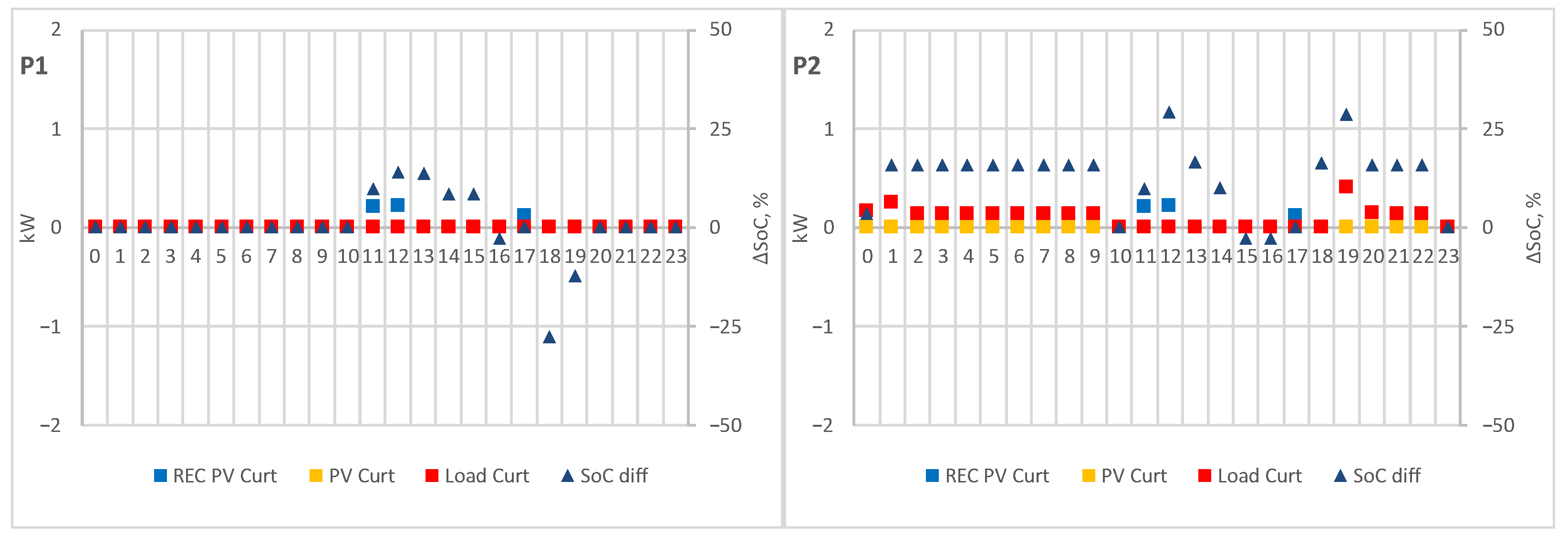
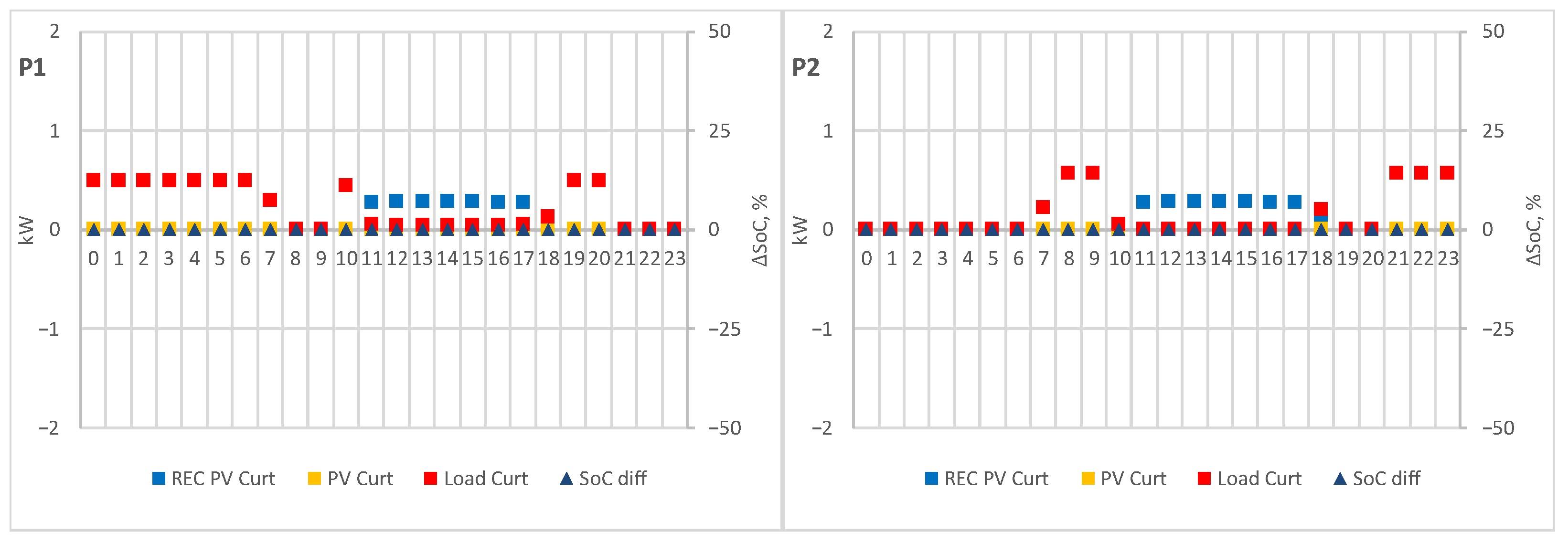
4.7. Scenario VII (Stage Three)

Further limiting the voltage to the window $0.95\le V_{i,t}\le 1.05\left(\mathrm{p}.\mathrm{u}.\right)$, as in the ANSI C84.1, increases the flexibility activation of stage three, with additional load and generation curtailment, and battery re-scheduling, as shown in Figure 21 and Figure 22. Prosumer P1 load curtailment amounts to 5.6 kWh or 23% of its total load, while P2 amounts to 3.3 kWh or 14%. External PV generation curtailment amounts to 4.2 kWh or 35% of the total generation. The flexibility cost is further increase to EUR 0.59. Again, flexibility activation is driven by the overvoltage observed at bus seven, this time residing at the limit of 1.05 p.u., as shown in Figure 23.

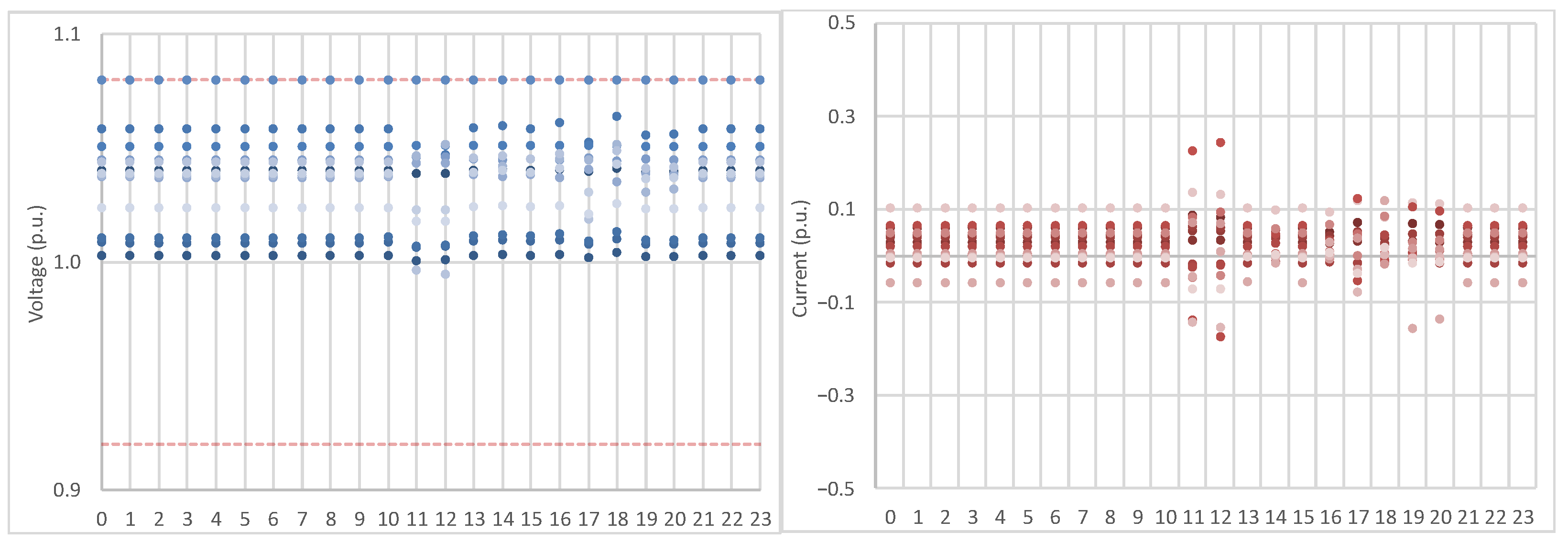
4.8. Scenario VIII (Stage Three)

To evaluate the impact of the batteries in the provision of flexibility, the schedules found in scenario VII where kept fixed in this scenario. As a result, the flexibility cost slightly increases from EUR 0.59 to EUR 0.60. We observe an additional load curtailment at P1 of 0.1 kWh (amounting to a total load curtailment of 5.7 kWh), the same load curtailment at P2 and the same external PV generation curtailment that results from re-arranging the curtailment schedule along all 24 h, with some hours showing an increase at both prosumers, and for others a decrease (compare Figure 24 and Figure 21). No generation curtailment was verified. Figure 25 also confirms that the batteries schedules remain equal to those of stage two, and Figure 26 shows that the voltages on all buses remain within the specified limits. This confirms that batteries are rescheduled in stage three to contribute to solve the grid constraints and to lower the flexibility activation costs, although their contribution is relatively small for this scenario.

5. Conclusions

This paper presents a three-stage model for the energy management of a renewable energy community. The first stage minimizes each peer’s costs, the second the overall community costs and the third stage incorporates an OPF to compute the most cost-efficient flexibility activation to solve existing grid constraints. The first stage allows the inclusion, in the second one, of a constraint to avoid increasing the cost of any prosumer when optimizing the community, which helps to make a fairer share of the collective benefits of a global optimization. Stages one and two can implement an automatic community control system or simulate the outcomes of a local energy market.

A settlement framework, based on the current self-consumption allocation rules of Portugal, is proposed to guarantee that the local activation of flexibility and the local energy transactions are adequately settled with retailers and aggregators at the wholesale market, and that the peers’ flexibility is properly compensated. Indeed, peer flexibility provision is smoothly integrated with the local energy market, and peers are financially compensated for this flexibility according to their energy cost increment, which depends on the tariffs with their retailers and the self-consumption tariffs, and on their utility or loss of comfort.

Several case examples have been provided, and their analysis has allowed to draw some interesting conclusions:

• Real allocation coefficients provide competition at the retail market, allowing some peers of the community to profit from other peers’ better tariffs, and improve the REC collective benefit. Indeed, these coefficients allow, for example, that peers with better supply tariffs share energy from their supplier (not locally generated) with other peers, reducing their energy bill;
• However, this may be harmful for some peers if the internal price does not compensate properly their internal supply. Internal prices should pay for the energy they buy from their suppliers and share internally, since, otherwise, they will incur in losses with respect to not being part of the energy community. Indeed, different prices could exist for these transactions and for those to share the energy generated locally. However, note that in a real market environment, no collective optimization would be performed, and peers would set their bid prices according to their opportunity costs and expectations for market outcomes to obtain the proper compensations for their internal transactions;
• If the regulation only accepts positive allocation coefficients, internal exchanges are significantly limited, reducing the competition at retail level since peers cannot share energy not produced locally. Even so, those peers with better tariffs can share all their local generation, increasing their consumption from their suppliers if they are properly compensated to reduce other peers’ energy bill;
• When a central management of the energy community is performed, the price fixed for the internal transactions has a direct impact on the optimization and the resulting self-consumption. Indeed, if the price is not fair, the constraint from the stage one significantly limits the transactions to avoid harming peers but leads to a lower community efficiency that will have a higher total energy cost. Therefore, a proper internal price is essential to maximize the self-consumption by allowing a fair energy sharing;
• Alternatively, stage two could be performed without stage one’s constraint, but then, an additional mechanism to share the collective benefits should be provided, either by designing a fair price computation methodology, or through some other mechanisms such as the Shapley value [15] or marginal contribution rule [16];
• Note that a market-based mechanism instead of central management would dramatically simplify the problem of sharing the collective benefits by passing the responsibility and complexity to the peers. However, the peers would need to design efficient bidding strategies to guarantee fair compensations to their internal transactions;
• When the grid constraints are considered, results from stage three confirm that the flexibility needed to solve grid problems is activated, leading to a flexibility cost to be compensated to the prosumers providing this flexibility. It is also interesting to highlight how re-dispatching the batteries in stage three contributes to solve the grid problems and to reduce the flexibility cost.

The authors are currently working on testing other sharing mechanisms for the collective benefits of the energy community and on simulating a local market based on the opportunity cost of peers to determine a fair price to be used in stage two.