Abstract
Water injection in geothermal areas is the preferential strategy to sustain the natural production of geothermal resources. In this context, monitoring microearthquakes is a fundamental tool to track changes in the reservoirs in terms of soil composition, response to injections, and resource exploitation with space and time. Therefore, refined source characterization is crucial to better estimate the size, source mechanism, and rupture process of microearthquakes, as they are possibly related to industrial activities, and to identify any potential variation in the background seismicity. Standard approaches for source parameter estimation are ordinarily based on the modelling of Fourier displacement spectra and its characteristic parameters: the low-frequency spectral level and corner frequency. Here, we apply an innovative time domain technique that uses the curves of P-wave amplitude vs. time along the seismogram. This methodology allows estimation of seismic moment, source radius, and stress release from the plateau level and the corner time of the average logarithm of P-wave displacement versus time with the assumption of a triangular moment rate function, uniform rupture speed, and a constant/frequency-independent Q-factor. In the current paper, this time domain methodology is implemented on a selected catalog of microearthquakes consisting of 83 events with a moment magnitude ranging between 1.0 and 1.5 that occurred during a 7-year period (2007–2014) of fluid extraction/injection around Prati-9 and Prati-29 wells at The Geysers geothermal field. The results show that the time domain technique provides accurate seismic moment (moment magnitude) and rupture duration/radius estimates of microearthquakes down to the explored limit (M 1) while accounting for the anelastic attenuation effect in the radiated high-frequency wavefield. The retrieved source radius vs. moment scaling is consistent with a self-similar, constant stress drop scaling model, which proves an appropriate attenuation correction and the validity of the assumed, triangular moment rate function for microearthquake ruptures. Two alternative mechanical models are proposed to explain the observed difference (about two orders of magnitude) in the retrieved average stress release estimates between the time and frequency domain methods. We argue that the two quantities may not refer to the same physical quantity representing the stress release of earthquake ruptures. Either the smaller stress release values from the time domain method may indicate a larger fracture area (by a factor of 20) radiating the observed P-waveforms than the one estimated from the corner frequencies, or the frequency domain estimate is a proxy for dynamic stress release while the time domain is more representative of the static release. The latter is associated with a much lower dynamic friction value than static friction value at the fault during the rupture process.
1. Introduction
In geothermal fields exploited for energy production, micro-seismicity can occur, caused by the reactivation of pre-existing faults and fractures by fluid extraction/injection during geothermal operations. In a vapor-dominated reservoir, fluid is injected into the subsurface under carefully controlled conditions, which cause pre-existing fractures to re-open, increasing steam production. The controlled hydraulic stimulation activity by periodic fluid injection causes the reactivation of the fracture network leading to an increase in permeability. The monitoring of induced earthquakes caused by fluid injection is currently a topic of great concern [1], not only for the development of more sophisticated techniques for the continuous control of geothermal operations but also to mitigate the effects of the increasing seismic activities which often raise panic among the population living close to geothermal areas [2] and, less frequently, can cause associated shaking and minor to moderate building damage [3,4]. In this study, we focus attention on The Geysers geothermal field (TG), located in northern California, which is the widest geothermal area in the world. It has been operating since the 1960s and contains the largest power plant in the world. Many studies have proved that the seismicity at TG is correlated with injection operation [5,6]. In particular, background seismicity is governed by thermoelastic and poroelastic effects that change the local stress field and spatiotemporal changes in fault regimes. Event occurrence and their source characteristics are linked to the injection rates [7]. It has been proven that the triggered micro-earthquakes tend to cluster around injection wells, where water is present in liquid form. Moreover, the average distance of seismicity from the wellbore increases significantly when the injections reach their peak. As the injected water descends, the capacity to trigger earthquakes is mostly governed by the water-rock temperature contrast which induces a plume of seismicity streaming down from the well [8,9]. Fluid migration also reflects in earthquake size distribution. Indeed, studies of b-value variations have shown that it is more likely to have a bigger magnitude far from the injection points [10,11]. The reason behind such a distribution lies in the fact that failure occurs when the effective normal stress decreases due to the increase in pore pressure by fluid injection [12]. Particularly, when a hot rock volume is already near failure, even a small increase in pore pressure can trigger ruptures [8]. Many observations have pointed out a strong dependence of the Brune stress drop on distance from the injection wells. Low stress-drop regions surrounding injection points correspond to high pore pressure perturbation and vice versa. In geothermal areas, the Brune stress drop could be used as a proxy for monitoring changes in pore pressure variation during hydrofrac operations [13]. Therefore, refined source characterization is crucial to better understand the history of rupture which in such areas is fundamental to keep track of the changes in background seismicity.
Standard approaches for source parameter estimation are based on spectral analysis of P- and S-wave signals. By modelling spectral shapes in the frequency domain, it is possible to calculate the seismic moment and the corner frequency from which moment magnitude, source radius, and static stress drop are inferred [14,15]. The seismic moment, for example, is estimated from the low frequency amplitude of displacement spectra. The source radius is typically obtained from the spectral corner frequency [16,17] and the static stress drop is derived from the relationship between two estimated quantities, through the Keilis-Borok (1959) relationship [18]. These procedures assume body-wave radiation from circular/rectangular fault ruptures so that the parameters can directly be related to the low-frequency level and corner frequency of spectra [14,19,20]. In principle, spectral techniques can be applied either on the P-wave or on the S-wave, provided that distinct phases are not mixed and that the proper portion of signals is selected. Indeed, one of the major issues related to the use of spectral techniques is that the results are very sensitive to the time window used for the analysis. This time window, if not properly selected, may result in the inclusion of instrumental noise and secondary phase arrivals, in addition to the direct waves, which may contaminate the estimation of spectral parameters. In addition to that, to obtain reliable source parameters, proper corrections for anelastic and site effects need to be applied and at a first order in the frequency domain. This is done by assuming an omega square spectral model from which effects of attenuation are eliminated through spectral ratios [21,22]. Moving towards micro to small seismicity, other limitations of spectral analysis may be encountered. Firstly, due to the fact that radiated energy from S-waves is typically larger than the P-waves, the latter could be more easily hidden in instrumental noise, resulting in some bias for the phase identification. Secondly, a high quality of recording data and a sufficiently high sampling frequency (a minimum of 300 Hz is required considering micro to small earthquake frequency content spans between 10 and 100 Hz) of the acquisition systems are required to ensure the proper measurement of source parameters [23]. Moreover, the source parameters are linked to the spectral corner frequency, fc, directly or through fitting inversions. The correct identification of corner frequency is crucial for the correct evaluation of stress drop, which might result in high bias when fc is not properly retrieved from spectral shapes.
In this study, we apply a time domain technique to characterize the natural and man-induced microearthquake source parameters [24]. The methodology provides the estimation of source parameters from the analysis of P-wave signals in the time domain. The main idea is based on the average logarithm of P-wave displacement (LPDT curve), in which the main features, the corner time and the plateau level, correlate to the duration and the peak of a triangular-modelled source time function. These curves have been used to quickly obtain the earthquake magnitude and the expected rupture length, supporting the hypothesis that the initial rupture behavior depends on the final earthquake size [25,26]. We work on a set of TG events with a moment magnitude between 1.0 and 1.5, localized around Prati-9 and Prati-29 injection wells. We build the LPDT curves for all the events to infer the corresponding source parameters, and then compare our results with the ones obtained by Kwiatek et al. [27] for the same dataset to which they applied a refined spectral technique that consisted of using the spectral fitting method on the observed ground velocity spectra, followed by using the mesh spectral ratio technique in order to reduce attenuation effects. The difference relies on the Kwiatek et al. method, requiring the calculation of a Fourier transform to estimate the parameters through a smooth spectral model (Brune-type), while our estimate is performed in the time domain specifically considering a triangular function for the P-displacement waveform radiated by the source. In the frequency domain method, to improve the frequency resolution, a sufficiently long time window must be selected that can possibly include secondary, multi-path arrivals in the analyzed signal. The source time duration, from which the source radius is obtained, is derived by the corner frequency which typically trades-off with other spectral parameters such as the attenuation parameter (t*) and the high frequency spectral decay parameter. The correction for anelastic attenuation is critical for both time and frequency domain methods, since it can significantly affect the source moment and duration estimate. One advantage of the frequency domain method is that seismic moment is derived from the low-frequency displacement on the spectral level, while the peak and duration amplitude of the triangular source time function are needed for the moment estimate in our time domain method. The main advantage of the time domain method is that it works on the source-radiated P-pulse (we are working on extending the method to S-pulses), so that the rupture radius is directly obtained from the displacement waveform half-duration without model assumptions.
2. Data and Methods
2.1. Data
Here, we selected a set of microearthquakes with a moment magnitude range of 1.0 to 1.5 which were located in the northwestern part of the TG area (Figure 1). Although the maximum moment magnitude available in our preliminary catalogue was 3.2, we decided to focus our attention on the smallest magnitude range because we are interested in exploring the lowest limit down to which the time domain technique is still applicable for source parameter determination. The events span a period of seven years, from 2007 to 2014, and are concentrated around two injection wells, Prati-9 and Prati-29. This amounts to a total number of 83 events analyzed in this study, which were also part of the cluster selected by Kwiatek et al. [27]. For each event, we selected the stations within a hypocentral distance of 5 km to avoid contaminations in waveforms, e.g., due to multi-path arrivals; thus, the final dataset consisted of a total number of 83 events (about 2000 waveforms) recorded by an average number of eight three-component short-period geophones per event. Location information is provided by the Northern California Earthquake Data Center (NCEDC) (available information at https://service.ncedc.org/fdsnws/event/1/, accessed on 1 January 2023).
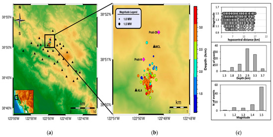
Figure 1.
(a) Map view of the TG area. The black triangles mark the location of the network stations. The black square highlights the area of the selected events. In the bottom left panel, the black square identifies the overall TG area in California; (b) Zoomed-in view of panel (a) for the selected events. Every event is marked with a circle whose size scales with magnitude, while the colors follow depth information according to the color bar on the right. The pink diamonds specify the locations of Prati-9 and Prati-29 wells. The two closest stations are marked with black triangles; (c) Top: number of records as a function of hypocentral distance; middle: depth distribution; bottom: magnitude distribution.
The majority of the events occurred at a depth of less than 3 km, and the maximum hypocentral distance was around 20 km.
2.2. Methods
In this paper, we applied the method proposed by Zollo et al. [24] for source parameter estimation, which relies on the evaluation of the logarithm of the peak displacement amplitude of high-pass filtered P-wave signals (LPDT curve). To this end, we used EASOt-AP, an open-source MATLAB package developed by Nazeri and Zollo [28]. Previous studies have shown that LPDT curves can be used as a proxy of the apparent source time function (STF) (Figure 2 in Nazeri et al. [29]). Indeed, LPDT curves show a characteristic behavior, with an initial monotonic increase starting from P-arrival up to a corner time where a flat level begins. We denote the corner time and plateau level with Tc and PL, respectively. These two parameters are correlated to the half-duration and the relevant amplitude of the isosceles triangular source time function which is here used to model the rupture process [24]. From Tc and PL, it is possible to obtain the area, Ωo, beneath the isosceles triangle linked to the integral of the far-field P-wave displacement radiated from a point source in a homogeneous, elastic, and half-space earth model as (more detail in [24]):
where Fs and Rθφ are the free surface factor and the radiation pattern coefficient related to the P-wave phase, respectively, M0 is the seismic moment, is the density of the area, R is the hypocentral distance, and Vp is the average P-wave velocity of the crustal volume under study. In the TG area, spatio-temporal variation in the VP/VS ratio correlates with the volume of water during injection operations, due to the increase in fluid saturation in reservoir rocks [30]. Considering the time period spanned by our dataset, we fixed the average value of VP = 5000 m/s, Vp/VS = 1.68, and = 2700 kg/cm3. These velocity and density values are inferred from the works of Gritto and Jarpe [30] and Guo and Thurber [31], respectively. This choice was made to have the same parameter settings as Kwiatek et al. [27]. In the hypothesis of a circular rupture with uniform velocity, VR, the source radius, a, can be obtained from the average half duration value of the source time function as follows [24]:
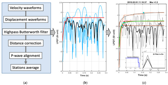
Figure 2.
(a) Working diagram for LPDT curve creation. After the integration of raw data (velocity waveforms) to get displacement waveforms, they were high-pass Butterworth filtered (fc = 0.5 Hz). Then, every station curve was corrected by hypocentral distance, aligned with reference to the first P-wave arrival time, and then averaged to obtain the LPDT event curve; (b) The blue lines represent station curves; the solid black line is the average of station curves; and the solid red curve is the LPDT curve for one event; (c) The orange curves are the ±1-sigma curves with respect to the red solid curve; the blue cyan circles refer to Tc; and the green line is the theoretical curve obtained with the retrieved Tc and PL. The bottom panels show the decrease in the number of stations with respect to the chosen time window (left bottom panel) and the triangular source time function built before (solid black line) and after (dashed black line) the Q-correction of Tc and PL (right bottom panel).
For a circular rupture model, a typical value for rupture velocity is 0.9 vs. [16,17].
Once the seismic moment, M0, and source radius, a, are available, the stress release, Δσ, is inferred through the formula [18,24]:
In order to obtain source parameters, LPDT curves are built for the events of the dataset. This approach shares the concept with the standard spectral analysis where signal spectra are processed to obtain corner frequency and a low asymptotic level which are related to source parameters. LPDT curves are built according to few steps which can be summarized in panel (a) of Figure 2. Firstly, velocity waveforms are integrated to obtain the displacement. To avoid the baseline effect, displacement waveforms are filtered with a high-pass cut-off frequency, fc = 0.5 Hz. Following the method by Zollo et al. [24], the LPDT curve at time t is evaluated as:
where t0 is the first P-arrival at a station at hypocentral distance R. Similar to the standard approaches for spectral techniques, we selected an appropriate P-wave time window to compute the LPDT curves. An appropriate selection of the time window strongly relates to the first P-wave arrival with respect to which LPDT curves are evaluated. It is crucial to be as accurate as possible in determining the first arrival. Given the small range of magnitude, we set the maximum time window, t, at 0.3 s, as an adequate amount of time for source time function modelling to be fully complete. The panels (b) and (c) of Figure 2 show an example of an LPDT curve for one of the events of our dataset. Once the curve is built, we performed fitting operations to obtain the corner time, Tc, and the plateau level, PL. In this work, we modelled the curves with a new function that simulated in the time domain a behavior similar to the high-pass Butterworth filter magnitude spectrum in the frequency-domain. The fit function used to model the LPDT curves in our study can be written as:
where Tc, PL, and γ are the curve-fitting parameters to be estimated. In particular, the latter describes the steepness of the increasing part of the LPDT curve. Here, y0 is constrained to the first point of the curve at time t0. From the analysis of each curve, we take Tc and PL to invert (1), (2), and (3) to obtain seismic moment, source radius, and stress release of each event. Note that up to this point, the anelastic attenuation has not been taken into account. The main effect of anelastic attenuation on seismic signals is a broadening of the pulse duration and a decrease in its amplitude. Standard approaches to include the attenuation effects would require the deconvolution of each station signal by the attenuation operator before the evaluation of LPDT curve. However, here we use a less invasive and time consuming technique; the half-duration and peak amplitude of the attenuated source time function is obtained through a global search that recursively simulates attenuated triangular source time functions for a set of recording stations with a given triangular source parameter couple, Tc and PL, with a known value of the quality factor, Qp. In fact, the way in which the anelastic attenuation correction is implemented requires the ‘a priori’ knowledge of the Q-factor in the area of interest. Moreover, the Q-factor is considered as a frequency-independent constant. TG area tomographic studies have revealed strong variations in Qp from the northern to the southern region. These variations are mostly attributed to differences in fracturing and fluid saturation. Moreover, at depths of ~2–4 km, there is a low Qp zone which is caused by the large amount of injected fluids in the surface [31,32]. Considering the depth distribution of our data set (Figure 1c), we set Qp = 100 ± 50.
3. Results
The source parameters obtained in this study for the selected dataset are shown in Figure 3 and Table A1, after the Q-factor correction using a value of Qp = 100 previously estimated for the TG area [32]. In Figure 3a, we compare the logarithm of seismic moments obtained with our methodology to the ones available in Kwiatek et al.’s [27] refined catalogue and obtained by the inversion of P-velocity spectra. The two quantities follow the one-to-one linear trend (shown with black solid line) within error. Therefore, in the explored magnitude range, this method can provide reliable moment magnitude estimates. Figure 3b shows the logarithm of rupture duration estimated after the Q-factor correction versus the logarithm of the seismic moment. The expected theoretical trend is 24, which is closely comparable with the current observation (). The source radius shows a linear trend with seismic moment in the log-log scale (Figure 3c) with a slight moment increase, as expected for a near constant stress drop scaling of the source size with moment. The average value of the stress release for this dataset is about 0.01 MPa (Figure 3d), which is about two orders of magnitude smaller than the average static stress drop value measured by Kwiatek et al. [27].
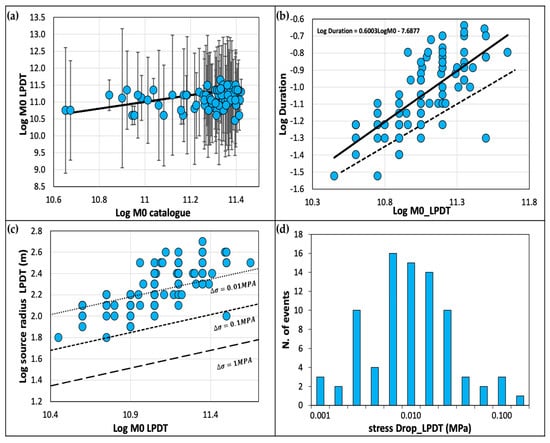
Figure 3.
(a) Logarithm of seismic moments obtained from LPDT versus logarithm of seismic moments available from Kwiatek et al.’s refined catalogue. The solid black line represents the one-to-one relationship of catalogue M0. The errors are obtained by error propagation from Tc and PL; (b) Logarithm of duration (inferred by Tc of LPDT curves) versus logarithm of M0 from LPDT. The solid black line of best fit is represented with its equation written in the top left corner of the panel; the dashed line represents the theoretical line with a slope value of 0.5 (see also Figure 4c [24]); (c) Logarithm of source radius versus logarithm of M0 from LPDT. The data show a constant stress drop scaling with an average value of 0.01 MPa. Following different line styles, three different fixed values of constant stress drop are represented in the graph; (d) Stress release distribution obtained from LPDT. The mean stress release value is around 0.01 MPa.
4. Discussion
The implemented time domain method for source parameter estimation has been successfully applied in previous works for various tectonic areas and to various moderate to large events [24,29]. Here, we applied the procedure on a micro to small magnitude (from 1 to 1.5 moment magnitude) dataset and retrieved reliable measurements even for such a small magnitude range (Figure 3). As for the seismic moment and moment magnitude, our results show a good match to those estimated with spectral techniques, where this is inferred from asymptotic low frequency spectral level of displacement records. Indeed, our estimates validate the triangular-shaped function used to model the relevant moment rate function of the earthquakes. The procedure is followed by varying the Q-factor within the range of values of the area of interest. The results are shown in Table 1, proving that the choice of Qp slightly affects source parameters given the investigated distance range. The lower the Q value, the higher the average stress release. In principle, the stress release is obtained from Equation (3) and ultimately depends on plateau level, PL, and corner time, Tc, so that the correction of the anelastic attenuation is affecting the peak and the half-duration of the modelled STF. From Equation (3), it is evident that the stress release essentially depends on the other two inferred parameters of seismic moment and source radius. Moreover, in the source parameter estimation, the role of rupture velocity cannot be ignored, which is strongly linked to the calculation of the rupture radius and hence stress release (Equations (2) and (3)). Here, we first fixed the rupture velocity at 0.9 vs. to exactly correspond to the parameter values of Kwiatek et al. [27] and to make a reliable comparison. However, to evaluate the dependency of the stress drop parameter on rupture velocity, later we changed this value to 0.6 vs. (Table 1). It is clear that any changes in the rupture velocity value correspond to a change in the average stress release for the whole dataset. In particular, the lower the VR, the higher the average stress release (particularly we found an average stress release value of 0.1 MPa considering a rupture velocity of 0.6 VS; this stress release value lowers to 0.01 MPa considering a rupture velocity of 0.9 VS). Compared to the spectral measurements made by Kwiatek et al. [27], our moment-source radius scaling is in better agreement with the expected theoretical scaling (Figure 4). The fact that the self-similar, constant stress drop scaling is preserved with our time domain technique validates the Q-correction of the modelled source time function.

Table 1.
Two different values of rupture velocity and three different values of Q have been tested to show changes in the average stress release value and in the average duration obtained from Tc measurements.
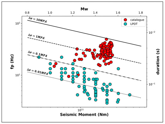
Figure 4.
Representation of frequency and duration (left and right axis) versus moment magnitude and seismic moment (upper and lower axis). The cyan points are the parameters obtained with the LPDT method, while the red points are the parameters from the refined catalogue of Kwiatek et al. [27]. Different values of stress drop are shown on the graph. It is visible that data from the LPDT method follow a better constant stress drop scaling.
Finally, the average stress release that we measured in the time domain was two orders of magnitude smaller than the one measured in the frequency domain by Kwiatek et al. [27], i.e., 0.01 MPa vs. 1 MPa. Different studies on stress drop variations in geothermal sites are in accordance with the results of the spectral analysis. Tomic et al. [33] concluded that the stress drop in small reservoir-induced earthquakes was similar to or higher than naturally occurring earthquakes, with values spanning from about 20 MPa up to 200 MPa. However, Goertz-Allmann et al. [13] found much smaller values for the Basel geothermal area with values in the range of 0.1–1 MPa at short distances from the injection well point. They concluded that the stress drop depends on pore pressure, and the lowest stress drop regions are the ones closest to the injection wells. Moving from a radial distance of 10 m to 300 m from injection points, the stress drop increases by up to a factor of five. The average stress drop found by Goertz-Allmann et al. [13] was still a hundred times larger than ours.
The discrepancy between the stress drop parameter measurements in the time and frequency domains can be possibly related to an overestimation or underestimation of the rupture duration for each method, respectively. Note that in both time and frequency domains, the stress drop parameter estimation is strongly affected by any error in corner time or frequency identification. Additionally, this discrepancy can be caused by the Qp value, which may be smaller than the one we decided to use. Looking at the values of the average duration obtained from corner time, Tc, for all events (Table 1), the smallest value of Qp (50) was still not able to justify such a discrepancy between the estimations of stress drop parameter. In Figure 4, we plot both the frequencies and the durations obtained from our procedure and the ones of Kwiatek et al.’s [27] refined catalogue. What is possible to observe is that the source durations derived from corner frequencies are smaller (with a mean value of 0.03 s) than those obtained by the LPDT method (with a mean value of 0.05). In fact, the average value of 0.03 s derived from corner frequencies is not consistent with the LPDT shapes and related corner time, since it occurs at the middle of the initial rise part of LPDT curves and well before reaching the plateau level. We therefore conclude that it is likely that the two durations derived from corner frequency and corner time might represent different parameters of the rupture process. One explanation may refer to the different portions of the P-wave radiating fault area resulting in a difference between the durations and consequently in the observed difference in stress drop parameter estimates. Corner frequencies are more sensitive to the characteristic subevent size, meaning that small patches of the whole fracture area are more likely to be estimated from measurements made through spectral techniques [34]. The overall fault area is in turn better represented by corner time, Tc. An alternative explanation is that the two values of stress drop parameter do not represent the same stress release quantity. Particularly, corner frequencies might represent proxies of the dynamic stress drop, while time durations are more linked to the static stress drop [14,17,34]. The fact that the dynamic stress drop is much higher that the static stress drop would imply a nearly zero dynamic friction during the rupture process and a sudden recovery (less than 0.1 s for fractures with a one hundred meter radius) of the static friction after the dynamic rupture. Beeler et al. [35] concluded that a dynamic stress drop higher than the static stress drop implies a positive overshoot and very small radiation efficiency, e.g., a large part of the fracture energy is spent for anelastic processes at the source rather than being converted to radiated waves.
5. Conclusions
We applied a time domain technique that uses the curves of P-wave amplitude versus time to estimate the source parameters of a set of 83 microearthquakes at The Geysers geothermal field with a moment magnitude ranging between 1.0 and 1.5. We found the following:
The time domain technique provides accurate seismic moment (moment magnitude) and rupture duration/radius estimates of microearthquakes down to the explored limit (M 1) while accounting for the anelastic attenuation effect of the radiated high-frequency wavefield, confirming the validity of this approach for such small magnitude events.
The retrieved rupture duration/radius estimates are consistent with a self-similar, constant stress drop scaling with seismic moment, which is evidence for an appropriate attenuation correction and the validity of the assumed, triangular moment rate function. A similar scaling is not observed for corner frequency-derived rupture radii for the same earthquake dataset, which can be related to a larger uncertainty affecting frequency domain measurements.
The estimated average stress release is about two orders of magnitude smaller than the one obtained from a spectral technique in the frequency-domain. We argue that the two quantities do not refer to the physical quantity representing the stress release of earthquake ruptures. Since the difference relies on the rupture radius estimates (a ratio of about 4.5), larger stress release values from the time domain method may indicate a larger fracture area (by a factor of 20) radiating the observed P-waveforms than the one estimated from the corner frequencies, which are more sensitive to the radiation of localized high-slip patches along the fault surface. Alternatively, this difference can be explained as the frequency domain estimate being a proxy for dynamic stress release, while the time domain is more representative of the static release, with the latter associated with much lower dynamics than static friction values at the fault during the rupture process.
Author Contributions
Conceptualization, S.N., V.L. and A.Z.; Methodology, S.N., V.L., S.C. and A.Z.; Software, V.L. and S.N.; Validation, V.L. and R.R.; Formal analysis, V.L.; Investigation, S.N., S.C. and G.D.L.; Data curation, V.L. and R.R.; Writing—original draft, V.L. and S.C.; Writing—review & editing, V.L., S.N., S.C., R.R., G.D.L. and A.Z.; Supervision, S.C., G.D.L. and A.Z.; Funding acquisition, A.Z. All authors have read and agreed to the published version of the manuscript.
Funding
This work has been supported by the PRIN-FLUIDS project: “Detection and tracking of crustal fluid by multi-parametric methodologies and technologies” of the Italian PRIN-MIUR programme (Grant no. 20174X3P29). This work has also been funded by the Italian Ministry of University and Research and by the University of Naples Federico II, within the framework of the National Operative Programme (PON-AIM 218 AIM1834927–3).
Data Availability Statement
All data used to support this research are freely available. The source for the data is summarized as it follows: EPISODES Platform Seismic Catalog HQ, THE GEYSERS Prati 9 and Prati 29 cluster at link https://tcs.ah-epos.eu/?lang=it#dataview:dc:5cee7927-9542-3f9e-8af5-872fca99edb7; Northern California Earthquake Data Center (NCEDC), Lawrence Berkeley National Laboratory for seismic data catalogs and waveform data at link https://service.ncedc.org/fdsnws/event/1/.
Acknowledgments
The authors would like to thank the reviewers and the Editor for their comments that helped to improve the manuscript.
Conflicts of Interest
The authors declare no conflict of interest.
Appendix A
Table A1.
Source parameters estimates for the 83 events used in this work. Origin time, location, and local magnitude are inferred from an NCEDC bulletin. Remaining source parameters and their errors are evaluated through our time domain technique. In particular, source duration was obtained from Tc measurements of event LPDT curves.
References
- Ellsworth, W.L. Injection-Induced Earthquakes. Science 2013, 341, 1225942. [Google Scholar] [CrossRef] [PubMed]
- Gaucher, E.; Schoenball, M.; Heidbach, O.; Zang, A.; Fokker, P.A.; van Wees, J.-D.; Kohl, T. Induced seismicity in geothermal reservoirs: A review of forecasting approaches. Renew. Sustain. Energy Rev. 2015, 52, 1473–1490. [Google Scholar] [CrossRef]
- Deichmann, N.; Giardini, D. Earthquakes Induced by the Stimulation of an Enhanced Geothermal System below Basel (Switzerland). Seism. Res. Lett. 2009, 80, 784–798. [Google Scholar] [CrossRef]
- Ellsworth, W.L.; Giardini, D.; Townend, J.; Ge, S.; Shimamoto, T. Triggering of the Pohang, Korea, Earthquake (Mw 5.5) by Enhanced Geothermal System Stimulation. Seism. Res. Lett. 2019, 90, 1844–1858. [Google Scholar] [CrossRef]
- Majer, E.L.; Peterson, J.E. The impact of injection on seismicity at The Geysers, California Geothermal Field. Int. J. Rock Mech. Min. Sci. 2007, 44, 1079–1090. [Google Scholar] [CrossRef]
- Leptokaropoulos, K.; Staszek, M.; Lasocki, S.; Martínez-Garzón, P.; Kwiatek, G. Evolution of seismicity in relation to fluid injection in the North-Western part of The Geysers geothermal field. Geophys. J. Int. 2018, 212, 1157–1166. [Google Scholar] [CrossRef]
- Martínez-Garzón, P.; Kwiatek, G.; Sone, H.; Bohnhoff, M.; Dresen, G.; Hartline, C. Spatiotemporal changes, faulting regimes, and source parameters of induced seismicity: A case study from The Geysers geothermal field. J. Geophys. Res. Solid Earth 2014, 119, 8378–8396. [Google Scholar] [CrossRef]
- Stark, M.A. Microearthquakes—A tool to track injected water in the geysers reservoir. Geotherm. Resour. Counc. 1992, 17, 111–117. [Google Scholar]
- Stark, M. Seismic Evidence for a long-lived Enhanced Geothermal System (EGS) In the Northern Geysers Reservoir. Geotherm. Resour. Counc. Trans. 2003, 27, 727–731. [Google Scholar]
- Shapiro, S.A.; Dinske, C.; Langenbruch, C.; Wenzel, F. Seismogenic index and magnitude probability of earthquakes induced during reservoir fluid stimulations. Geophysics 2010, 29, 304–309. [Google Scholar] [CrossRef]
- Bachmann, C.E.; Wiemer, S.; Goertz-Allmann, B.P.; Woessner, J. Influence of pore-pressure on the event-size distribution of induced earthquakes. Geophys. Res. Lett. 2012, 39. [Google Scholar] [CrossRef]
- Rutledge, J.T.; Phillips, W.S. Hydraulic stimulation of natural fractures as revealed by induced microearthquakes, Carthage Cotton Valley gas field, east Texas. Geophysics 2003, 68, 441–452. [Google Scholar] [CrossRef]
- Goertz-Allmann, B.P.; Goertz, A.; Wiemer, S. Stress drop variations of induced earthquakes at the Basel geothermal site. Geophys. Res. Lett. 2011, 38, 2011GL047498. [Google Scholar] [CrossRef]
- Boatwright, J. A spectral theory for circular seismic sources; simple estimates of source dimension, dynamic stress drop, and radiated seismic energy. Bull. Seismol. Soc. Am. 1980, 70, 1–27. [Google Scholar]
- Supino, M.; Festa, G.; Zollo, A. A probabilistic method for the estimation of earthquake source parameters from spectral inversion: Application to the 2016–2017 Central Italy seismic sequence. Geophys. J. Int. 2019, 218, 988–1007. [Google Scholar] [CrossRef]
- Madariaga, R. Dynamics of an expanding circular fault. Bull. Seismol. Soc. Am. 1976, 66, 639–666. [Google Scholar] [CrossRef]
- Brune, J.N. Tectonic stress and the spectra of seismic shear waves from earthquakes. J. Geophys. Res. Atmos. 1970, 75, 4997–5009. [Google Scholar] [CrossRef]
- Borok, V.K. On estimation of the displacement in an earthquake source and of source dimensions. Ann. Geophys. 2012, 12, 205–214. [Google Scholar] [CrossRef]
- Savage, J.C. Relation between P- and S-wave corner frequencies in the seismic spectrum. Bull. Seism. Soc. Am. 1974, 64, 1621–1627. [Google Scholar] [CrossRef]
- Sato, T.; Hirasawa, T. Body wave spectra from propagating shear cracks. J. Phys. Earth 1973, 21, 415–431. [Google Scholar] [CrossRef]
- Masuda, T.; Suzuki, Z. Objective estimation of source parameters and local Q values by simultaneous inversion method. Phys. Earth Planet. Inter. 1982, 30, 197–208. [Google Scholar] [CrossRef]
- Ide, S.; Beroza, G.C.; Prejean, S.; Ellsworth, W.L. Apparent break in earthquake scaling due to path and site effects on deep borehole recordings. J. Geophys. Res. Solid Earth 2003, 108. [Google Scholar] [CrossRef]
- Kwiatek, G.; Ben-Zion, Y. Theoretical limits on detection and analysis of small earthquakes. J. Geophys. Res. Solid Earth 2016, 121, 5898–5916. [Google Scholar] [CrossRef]
- Zollo, A.; Nazeri, S.; Colombelli, S. Earthquake Seismic Moment, Rupture Radius, and Stress Drop From P-Wave Displacement Amplitude Versus Time Curves. IEEE Trans. Geosci. Remote Sens. 2021, 60, 1–11. [Google Scholar] [CrossRef]
- Colombelli, S.; Zollo, A.; Festa, G.; Picozzi, M. Evidence for a difference in rupture initiation between small and large earthquakes. Nat. Commun. 2014, 5, 3958. [Google Scholar] [CrossRef] [PubMed]
- Colombelli, S.; Festa, G.; Zollo, A. Early rupture signals predict the final earthquake size. Geophys. J. Int. 2020, 223, 692–706. [Google Scholar] [CrossRef]
- Kwiatek, G.; Martínez-Garzón, P.; Dresen, G.; Bohnhoff, M.; Sone, H.; Hartline, C. Effects of long-term fluid injection on induced seismicity parameters and maximum magnitude in northwestern part of The Geysers geothermal field. J. Geophys. Res. Solid Earth 2015, 120, 7085–7101. [Google Scholar] [CrossRef]
- Nazeri, S.; Zollo, A. EASOt-AP: An open-source MATLAB package to estimate the seismic moment, rupture radius, and stress-drop of earthquakes from time-dependent P-wave displacements. Comput. Geosci. 2023, 171, 105293. [Google Scholar] [CrossRef]
- Nazeri, S.; Colombelli, S.; Zollo, A. Fast and accurate determination of earthquake moment, rupture length and stress release for the 2016–2017 Central Italy seismic sequence. Geophys. J. Int. 2019, 217, 1425–1432. [Google Scholar] [CrossRef]
- Gritto, R.; Jarpe, S.P. Temporal variations of Vp/Vs-ratio at The Geysers geothermal field, USA. Geothermics 2014, 52, 112–119. [Google Scholar] [CrossRef]
- Guo, H.; Thurber, C. Double-difference seismic attenuation tomography method and its application to The Geysers geothermal field, California. Geophys. J. Int. 2021, 225, 926–949. [Google Scholar] [CrossRef]
- Guo, H.; Thurber, C. Temporal Changes in Seismic Velocity and Attenuation at The Geysers Geothermal Field, California, From Double-Difference Tomography. J. Geophys. Res. Solid Earth 2022, 127. [Google Scholar] [CrossRef]
- Tomic, J.; Abercrombie, R.E.; Nascimento, A.F.D. Source parameters and rupture velocity of small M ≤ 2.1 reservoir induced earthquakes. Geophys. J. Int. 2009, 179, 1013–1023. [Google Scholar] [CrossRef]
- Boatwright, J. Seismic estimates of stress release. J. Geophys. Res. Atmos. 1984, 89, 6961–6968. [Google Scholar] [CrossRef]
- Beeler, N.M.; Wong, T.-F.; Hickman, S.H. Effective Shear Fracture Energy, and Efficiency. Bull. Seismol. Soc. Am. 2003, 93, 1381–1389. [Google Scholar] [CrossRef]


Disclaimer/Publisher’s Note: The statements, opinions and data contained in all publications are solely those of the individual author(s) and contributor(s) and not of MDPI and/or the editor(s). MDPI and/or the editor(s) disclaim responsibility for any injury to people or property resulting from any ideas, methods, instructions or products referred to in the content. |
© 2023 by the authors. Licensee MDPI, Basel, Switzerland. This article is an open access article distributed under the terms and conditions of the Creative Commons Attribution (CC BY) license (https://creativecommons.org/licenses/by/4.0/).