Temperature-Dependent Ferromagnetic Loss Approximation of an Induction Machine Stator Core Material Based on Laboratory Test Measurements

Abstract

The accurate measurement and modeling of ferromagnetic material losses are vital issues during the design and analysis of electrical machines. Higher loss values can describe the manufactured rotor and stator machine plates better than the catalog data obtained by standardized measurements using the Epstein frame. In this paper, different temperature-dependent models based on the loss-separation principle are introduced and compared with the measurements. The model parameters are computed from customized laboratory and standardized measurements. The customized measurements based on the stator part of an induction machine in the range of the automotive industry standard, i.e., in [−40 $°$C, ⋯, 180 $°$C]. The proposed model and measurement process can be used in the post-processing stage of numerical field analysis to obtain electromagnetic losses according to the agreement between measured and simulated results. During a numerically expensive optimization process, this model can be used to consider the temperature dependence of the losses more accurately. The study shows that more than 50% of loss increase can be measured, compared with the catalog data, if we use the manufactured, stator-based, customized measurements based on the estimation of the iron loss parameters.

1. Introduction

Electrical machines are critical components of e-mobility applications, for which the ferromagnetic cores are one of the primary sources of losses. Reducing the core losses and increasing the power density of the machines is one of the main goals during the design process. A novel trend in electrical machine manufacturing is to create a robust design that will be insensitive to manufacturing intolerances [1,2,3]. The robust design optimization procedure is numerically expensive, where the consideration of the tolerances on the main parameters of the machine significantly increases the number of calculated design cases. Moreover, the effect of small changes in the optimized parameters needs accurate numerical predictions and considerably more numerical calculations [4,5].

In ferromagnetic materials, the magnetic loss is based on Joule heating, which is generated by the motion of the magnetic domain walls [6,7]. Nowadays, most of the electrical machine design process contains finite element calculations. The most advanced calculation of the ferromagnetic losses can be made by those finite-element-based tools that use integrated mathematical hysteresis models (Preisach or Jiles–Atherton models), to directly estimate iron losses [8,9,10,11,12]. Despite the high accuracy of these methods, their applicability for example, in the conceptual design optimization phase, is limited due to their high numerical cost. Moreover, these methods need a relatively high knowledge of the applied material, and the exact shape of the B–H hysteresis loop, which usually needs measurement and can be affected by many factors [6]. These data are usually not available at the early design stage, when not only the geometric data but many other quantitative data are missing from the applied materials [13].

Most of the FEM tools use post-processing-based techniques to calculate the losses. These techniques contain measurement-based formulas, which approximate the loss as a polynomial function of the magnetic flux density. Many FEM tools use the loss separation model, which is based on the Steinmetz equation [14,15,16,17]:

$$P=C{f}^{\alpha }{B}^{\beta },$$

(1)

where P denotes the approximated losses, the frequency is denoted by f, and B means the amplitude of the magnetic flux density. The C, $\alpha$, and $\beta$ are model parameters that can be determined from the measured data. These model parameters should be calculated for every considered frequency harmonics separately. This model assumes that the excitation has a pure sinusoidal magnetic flux density waveform. During a FEM-based calculation, the time-dependent magnetic flux density values should be considered for every finite element. The losses are calculated element-wise by post-processing these time-dependent magnetic flux densities using Equation (1). This is a very easily applicable methodology, which can give accurate results when the magnetomotive force is sinusoidal. However, this condition is not fit for most modern electrical machine topologies and drive systems [1,5,15].

Jordan modified and extended the Steinmetz equation (Equation (1)) to improve its accuracy, with the consideration of the eddy current losses generated in laminated steel sheets [18]. This model assumes that different physical processes generate losses. It assumes that the sum of a static magnetic hysteresis and the eddy current loss of the laminations can calculate the losses:

$$P=P_{hyst}+P_{ec}=C_{h}f{B}^2+C_e{f}^2{B}^2.$$

(2)

Here, the first term represents the hysteresis losses ($P_{hyst}$), and the second term considers the newly introduced eddy current losses ($P_{ec}$). The model contains two parameters that must be fitted into measured loss data. These are $C_h$ and $C_e$. These iron-loss separation models assume that the hysteresis losses are proportional to the time-dependent magnetic flux density. This assumption is a weakness of this approach because the value of the hysteresis loss is not zero after a magnetization process at zero flux density. It can be seen that, in these cases, hysteresis-loss-approximation-based formulae generally over- or underestimates the momentary value of this term. Bramerdorfer proposed an improvement, a radial basis function-based nonlinear modeling technique, which uses the magnetic flux and its first-time derivative to consider the previous state of magnetization for the hysteresis loss estimation [15]. The eddy current loss term can be derived from Maxwell’s equations, and it can be written in the following form:

$$P_{ec}=\frac{\sigma d^2}{12\rho }{\left(\frac{dB\left(t\right)}{dt}\right)}^2,$$

(3)

where B(t) is the time-dependent value of the magnetic flux density, d is the thickness of the steel sheet, $\rho$ represents its specific mass, and the $\sigma$ represents the specific conductivity of the steel sheet. The Jordan model (Equation (2)) works well on a wide variety of nickel–iron alloys [6,7]. However, it is not accurate in the case of SiFE alloys, where a significant amount of excess loss was generated. These additional losses are usually described by a third term:

$$P=C_{h}f{B}^n+C_e{f}^2{B}^2+C_a{f}^{1.5}{B}^{1.5},$$

(4)

where the last term represents these additional excess losses. Bertotti introduced a statistic-based measure and a theory to calculate these excess losses [19]. He interpreted this excess loss factor ($C_a$) with the grain size of the magnetic domains and their wall motion:

$$C_a=\sqrt{S{V}_0\sigma G},$$

(5)

where $\sigma$ is the electric conductivity, S is the cross-sectional area of the lamination, $V_0$ takes the grain size and the local forces into account, and G is a material constant whose value is about 0.136 [7,20].

However, rotational losses affect iron losses in electrical machines. Many papers consider how these losses can be considered with the modified version of this formula (Equation (4)) [21,22,23]. The cutting and punching processes of the iron sheets significantly influence the material properties and create inhomogeneous stress in a narrow region of the core material. The thickness of this region is estimated using electron microscopy, and it is around 100–150 $\mathsf{\mu }$m, where the magnetic properties change significantly. Moreover, stacking and welding the iron sheets during machine core assembly also increases iron loss. All of these manufacturing processes increase iron loss, which must be considered in modeling and design [6,7,24]. This most commonly used iron-loss separation model (Equation (4)), or its modifications, is integrated into many commercial FEM tools. These tools usually use additional steps during the processing. For example, they use different frequency separation approaches to determine the losses. Nevertheless, these tools allow the users to define these material parameters for loss separation models using Equation (4).

There are two possible ways to calculate these model parameters. First, we can use the technical datasheet of the electrical steel, typically obtained by using a standard Epstein frame, and provide some maximum guaranteed values and typical average values of magnetic properties [6,7,16,17]. The main problem with iron loss measurement is that the catalog data can only partially estimate iron losses. The factory and standardized measurements are taken with a standard Epstein frame on relatively large lamination sheets with regular shapes cut from a stack of plates produced by rolling, regardless of the use of iron plates.

By contrast, stator elements usually contain many slots that are cut from iron plates. The impact of mechanical influences (e.g., cutting, joining) all modify the ferromagnetic material’s hysteresis characteristics and significantly affect the losses. Therefore, customized laboratory measurements will undoubtedly result in higher and more accurate loss calculations than standardized measurement-based calculations. Different methods can be used for these customized laboratory measurements; it can be used as an Epstein frame [16,17,25] or a toroidal-shaped core transformer [26], which can accurately take these extra losses into account during the design process.

The previously proposed models have their best performance at a constant temperature. Some recent research examined the temperature dependence of these iron loss parameters. The first group of the temperature-dependent iron-loss separation models assumed that the temperature affects the eddy current of the iron-loss model due to the temperature dependency of the electric resistivity [27]. In [22,28], the authors examined the temperature dependence of non-oriented silicon steel laminations till 100 °C. Their model assumed that the magnetic permeability of the examined steel depends on the temperature. Therefore, not only the eddy currents but also the hysteresis losses change by the temperature. The authors showed that both the hysteresis and eddy current losses change linearly as a function of the temperature.

This paper proposes a novel measurement setup that can examine the temperature dependence of an induction machine in a wider range, up to 200 °C, than discussed in previous studies, and a temperature-dependent model is given based on the loss separation principle and validated by the measurements. Moreover, this paper compares the losses calculated based on standardized Epstein frame measurements (catalog data) with the results from customized laboratory tests. It is shown that the loss in the examined stator is much higher due to the effects of manufacturing, and the customized laboratory-measurement-based calculations give a significantly better estimation for the losses. This paper aims to show a step-by-step approach to making a customized, ferromagnetic loss model that can handle temperature dependency for further optimization of the machine. The resulting ferromagnetic model can take the temperature dependency of a material during a 2D FEM-based optimization of the machine. The proposed model can be used in the post-processing stage of finite-element-method-based modeling to obtain losses in the core material.

2. Methodology

2.1. The Applied Iron-Loss Model

The electromagnetic loss of the ferromagnetic material (P) can be approximated as the sum of three main components: the hysteresis loss ($P_h$), the eddy current loss ($P_e$), and the anomalous loss ($P_a$) according to Bertotti’s loss separation model [6,29,30,31,32,33]:

$$P=P_h+P_e+P_a.$$

(6)

This model supposes that all of the separated losses can be expressed as a function of the exciting alternating magnetic flux density frequency f, and the amplitude of the magnetic flux density in the tested material B. In this paper, we use a modified formula to approximate the material-dependent coefficients. The previously shown equation can be expressed in the following way:

$$P=P(f,B)=k_{h}f{B}^{\alpha \left(B\right)}+k_e\left(B\right)f^2{B}^2+k_a\left(B\right)f^{1.5}{B}^{1.5},$$

(7)

where $k_h=k_h\left(B\right)$, $k_e=k_e\left(B\right)$, $k_a=k_a\left(B\right)$, and $\alpha =\alpha \left(B\right)$ represent the a priori empirical measurement-based coefficients of the hysteresis, eddy current, and anomalous losses. These coefficients are magnetic flux density-dependent functions in the proposed model. Using different modeling assumptions, these coefficients can be calculated from the measured data.

First of all, the coefficients are not supposed to be constant, and they are a function of the magnetic flux density amplitude. In our paper, two models were built [29,30,31,32]. The first approach contains all three components ($P_h$, $P_e$, and $P_a$), while in the second model, the last term ($P_a$) is skipped to achieve a simple representation. The first approach is an extended Bertotti-like model, while the latter is an extension of the Jordan model. Temperature dependency is taken into account only in the eddy current loss. The details are shown in Section 4.

As presented in [22,34], in order to take temperature dependence into consideration, one method is to consider the temperature dependency of eddy current loss only, thus assuming hysteresis loss and excess loss to be temperature-independent. The eddy current loss coefficient is related to the electrical resistivity as follows:

$$\rho \left(T\right)=\rho \left(20\right)[1+\vartheta (T-20\left)\right],$$

(8)

where T is the temperature, $\rho \left(20\right)$ is the resistivity at room temperature, $T=20°\mathrm{C}$, and finally, $\vartheta$ denotes the temperature coefficient. The insertion of this kind of model will be detailed in Section 4.

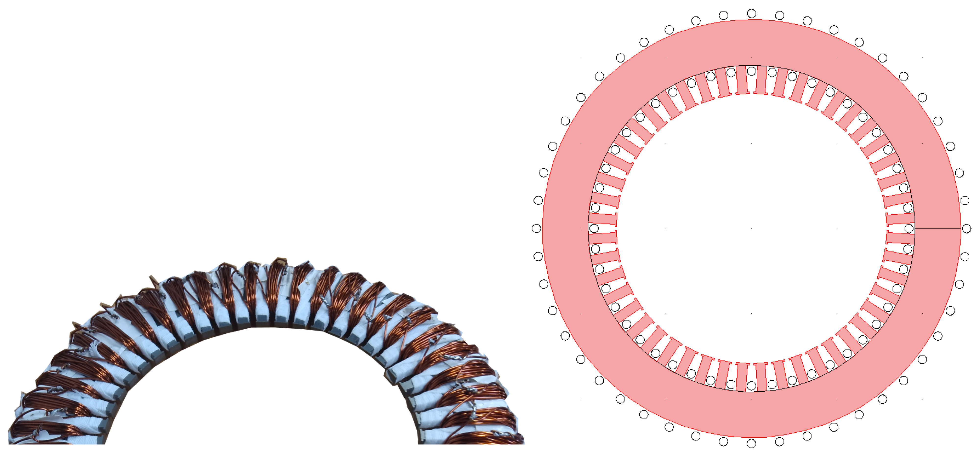
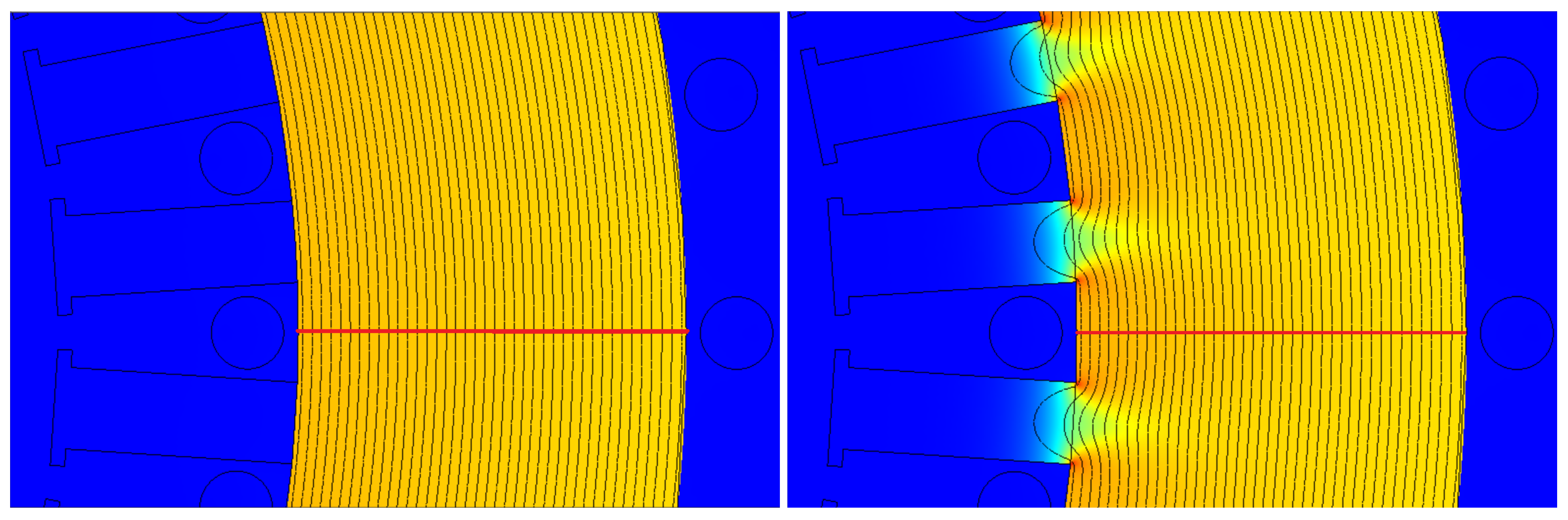
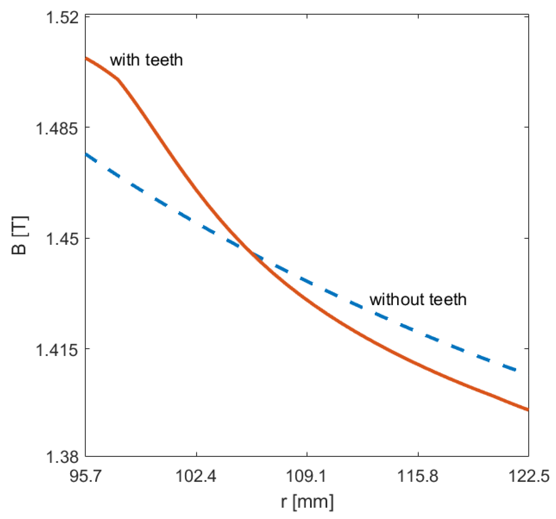
2.2. Finite-Element-Method-Based Design of the Measurements

After the numerical analysis-based design, the studied specimen was made of stator core material with feeding coils. The model for the two-dimensional analysis can also be seen in Figure 1. The inner diameter of the depicted stator core was 157 mm, the tooth height was 157 mm, and the outer diameter of the stator core was 245 mm.

Fourteen laminae from the stator part of the electric machine were removed to prepare a sample for the measurements. Measurement uncertainty can be reduced by measuring several plates stacked together, and the sample in this paper consisted of fourteen plates. The thickness of one lamination was 0.35 mm.

Before the measurements were carried out, the finite element method (FEM [35]) was used to perform simulations and map out what to expect qualitatively from the measurements. FEM simulations were carried out using COMSOL Multiphysics 3.5a [36]. A turns model was used for the coil supplying the magnetic field with a circular shape of a diameter equal to 5 mm. The eddy currents inside the ferromagnetic plate were neglected, and the two-dimensional magnetic field problem was solved using the magnetic vector potential formula [35]. The nonlinearity of the ferromagnetic plate was taken into account using the soft iron model of COMSOL Multiphysics 3.5a.

The idea was to round a coil on the stator yoke as if it were a toroid. An arrangement is a toroid if there are no teeth and slots (see Figure 2; left). It was not the goal to seal the teeth off to avoid mechanical impact. If there were teeth, the homogeneous magnetic field was slightly modified, as shown in Figure 2; right. It can be seen that the character was unchanged over most of the lamination pack, but some inhomogeneity developed near the teeth. FEM simulation was applicable to study the deviation according to the stator teeth. Figure 3 shows a typical variation in the magnetic flux density B along the red line of Figure 2. The difference between the magnetic flux density curves was a maximum of 2%.

After the comprehensive numerical field analysis, it can be stated that the stator teeth did not affect the measured magnetic field quantities, hysteresis curves, and finally, iron losses.

3. Measurement Results

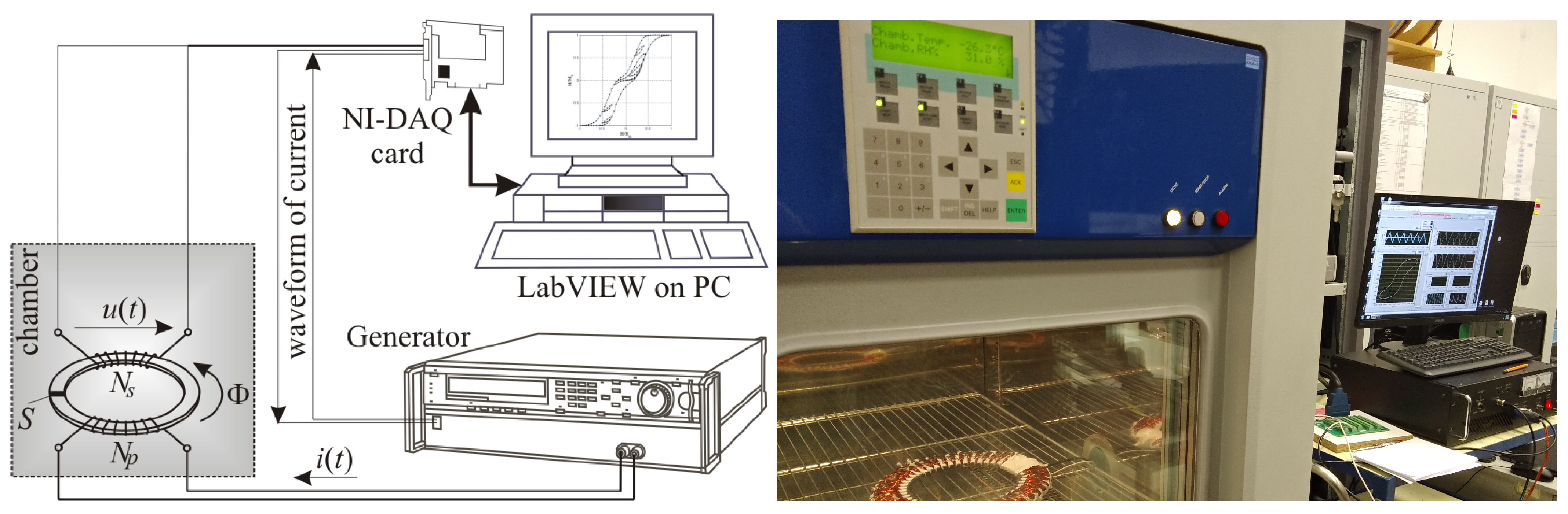
3.1. Measurement System

The specimen with the primary excitation coil consisting of 720 turns is shown in Figure 1. The exciting current can determine the magnetic field intensity $H=H\left(t\right)$. One slot contains a secondary coil with 20 turns made of thin wire. This secondary coil measures the magnetic flux density $B=B\left(t\right)$. Finally, the magnetic hysteresis characteristics of the ferromagnetic material can be drawn, from which the magnetic loss can be determined [26].

The details of the measurement system including the block diagram of the realized measurement arrangement and the photo of the measurements are shown in Figure 4. During the measurement of the iron loss characteristics, the turns ($N_p$ in Figure 4) of the primary winding can be excited with a predefined time function $i\left(t\right)$. This excitation induces an open-circuit voltage $u\left(t\right)$ in the open secondary winding of the transformer ($N_s$). The time function of the current and the induced voltage in the measurement setup can be measured using a National Instruments Data Acquisition (NI-DAQ) card. The signal waveform of the current can be sent to the generator via the same card. The measurement software developed in a LabVIEW environment runs on a computer, controls the entire measurement, regulates the current generator, measures and processes the incoming signals, and displays the measurement results.

The magnetic field intensity $H\left(t\right)$, the magnetic flux density $B\left(t\right)$, and the total electromagnetic loss P can be calculated as follows [37]:

$$H\left(t\right)=\frac{N_{p}i\left(t\right)}{l},B\left(t\right)=\frac{1}{S{N}_s}{\int }_0^{t}u\left(\tau \right)\mathrm{d}\tau ,P=\frac{1}{T\rho }{\int }_0^{T}H\frac{\mathrm{d}B}{\mathrm{d}t}\mathrm{d}t,$$

(9)

where l is the mean length, which is $l=684.5$ mm in the examined case, and S is the cross-section of the stator core. The mass density of the stator core material is denoted by $\rho$, and in the examined stator core plate $\rho =7600\mathrm{kg}/{\mathrm{m}}^3$, and T represents the examined time period.

The measurements were performed by setting the different amplitudes and frequencies of the magnetic flux density waveform. A chamber was set up with the desired core temperature.

3.2. The Examined Material and the Measurement Results

The stator plate was made of the ferromagnetic material M250-35A. In the first part of the notation, the letter M refers to magnetic steel, while 250 means that 2.5 W/kg is the maximum measured loss at 1.5 T magnetic flux density at a 50 Hz frequency. In the second part, 35 refers to the thickness of the plate, which was 0.35 mm in our case. The letter A at the end of the mark means applied rolling and fabrication type. The examined material was a cold-rolled, non-oriented electrical steel sheet without a specific magnetization direction.

The catalog data measured on a standard Epstein frame are given in

Table 1. The standardized, Epstein-apparatus-based catalog data for the examined ferromagnetic material M250-35A at all of the examined frequencies.

B [T]	H at 50 Hz (A/m)	P at 50 Hz (W/kg)	P at 100 Hz (W/kg)	P at 200 Hz (W/kg)	P at 400 Hz (W/kg)	P at 1000 Hz (W/kg)	P at 2500 Hz (W/kg)
0.2	35.7	0.06	0.14	0.33	0.90	3.65	14.8
0.4	47.5	0.21	0.51	1.23	3.24	12.7	51.7
0.6	60.0	0.41	1.01	2.49	6.69	26.3	113
0.8	77.5	0.66	1.64	4.12	11.2	45.7	208
1.0	107	0.98	2.41	6.14	17.1	72.6	352
1.2	179	1.37	3.4	8.69	24.6	-	-
1.4	642	2.00	4.83	12.4	35.1	-	-
1.6	4030	2.65	-	-	-	-	-
1.8	11,700	3.06	-	-	-	-	-

[38], where loss values for different amplitudes and frequencies of the sinusoidal magnetic flux density are listed. The second column also contains the value of the magnetic field intensity. The first magnetization curve, which shows the losses at 50 Hz, is plotted in Figure 5 with the red curve. The image contains our laboratory measurements at the same frequency at room temperature (20 °C), denoted by the blue color. It can be seen from the image that the red line fits well in the middle of the hysteresis loop; this indicates that there are no significant differences that can be measured in the magnetic permeability. In our case, the hysteresis loop area increased compared with the standardized measurements. This difference resulted in increased loss values.

Laboratory measurements were taken at the temperatures of −40 $°$C$,20°$C$,100°$C$,140°$C$,180°$C, and the following frequencies: 50 Hz, 100 Hz, and 200 Hz. This arrangement was because 200 Hz was the limit of the available current source generator.

Table 2. Measured loss values at room temperature.

B (T)	P at 50 Hz (W/kg)	P at 100 Hz (W/kg)	P at 200 Hz (W/kg)
0.2	0.11 (83%)	0.26 (85%)	0.71 (115%)
0.4	0.37 (76%)	0.91 (78%)	2.36 (92%)
0.6	0.66 (61%)	1.79 (77%)	4.65 (87%)
0.8	1.09 (65%)	2.91 (77%)	7.68 (86%)
1.0	1.44 (47%)	4.24 (76%)	11.28 (84%)
1.2	2.12 (55%)	5.79 (70%)	14.70 (69%)

presents the loss values measured at room temperature at different frequencies from 0.2 T to 1.2 T. The relative values of the catalog data are presented in parentheses after every measurement. Figure 6 plots the measured core loss parameters in the given layout compared to the standardized measurement-based catalog data. The laboratory-measured loss values and the standardized measurement-based catalog data were compared. It can be seen from the values that the stator plate measurement base loss values are significantly higher, at least 15%, due to manufacturing errors. 

Table 3. Measured loss values at 50 Hz and different temperatures.

B (T)	P at $-40°$C (W/kg)	P at 20 $°$C (W/kg)	P at 100 $°$C (W/kg)	P at 140 $°$C (W/kg)	P at 180 $°$C (W/kg)
0.2	0.12	0.11	0.09	0.09	0.09
0.4	0.39	0.37	0.36	0.32	0.30
0.6	0.72	0.66	0.68	0.65	0.65
0.8	1.12	1.09	1.09	1.09	1.05
1.0	1.67	1.44	1.64	1.49	1.43
1.2	2.19	2.12	2.02	2.01	1.97

presents the temperature dependency of the loss at 50 Hz under different temperatures. The catalog highlights two typical values at 50 Hz: the loss at 1.5 T is a maximum of 2.35 W/kg, and at 1.0 T, the loss is a maximum of 0.98 W/kg. The measured data are 3.42 W/kg, and 1.44 W/kg, respectively. We will use these values at the end of the paper for further characterization of the steel.

Figure 7 presents the measured losses (P) as a function of the magnetic flux density and the frequency, i.e., $P=P(B,f)$.

The loss slightly decreases by increasing the temperature. This result can be seen in Figure 8 with the values from Table 3. Ultimately, loss is a function of the magnetic flux density, the frequency, and the temperature, i.e., $P=P(B,f,T)$.

It is noted that measured loss values at very low frequencies are necessary for appropriate model fitting. Otherwise, the non-physical behavior of the model, i.e., negative loss values, may appear. This is why the loss was measured at 1 Hz (see

Table 4. The loss at 1 Hz.

B (T)	0.2	0.4	0.6	0.8	1.0	1.2
P (W/kg)	$1.9\times {10}^{-3}$	$5.8\times {10}^{-3}$	$10\times {10}^{-3}$	$15\times {10}^{-3}$	$21\times {10}^{-3}$	$30\times {10}^{-3}$

), and these values were assumed to be independent of the temperature because the values were very small.

4. Analysis of Characteristics in the Applied Ferromagnetic Loss Models

4.1. Characteristics of the First Analytical Approach

Because every measurement was performed on a fixed frequency, the model expression in (Equation (7)) can be simplified by dividing both sides of (Equation (7)) by the frequency f. Model identification becomes much easier through this reformulation.

The following formula is given:

$$\frac{P}{f}=k_h{B}^{\alpha }+k_{e}f{B}^2+k_a\sqrt{f}{B}^{1.5},$$

(10)

which can be rewritten as the second-order polynomial formula

$$\frac{P}{f}=p_0+p_1\sqrt{f}+p_2{\left(\sqrt{f}\right)}^2,$$

(11)

i.e.,

$$k_h=\frac{p_0}{B^{\alpha }},k_e=\frac{p_2}{B^2},k_a=\frac{p_1}{B^{1.5}}.$$

(12)

First, the polynomial coefficients $p_0$, $p_1$, and $p_2$ of (11) are fitted, from which the model parameters are obtained according to (12).

The measured loss P is plotted as the function of frequency, and $P/f$ is the root function of the frequency in Figure 8. The curves present P and $P/f$ values for different magnetic flux density amplitudes. The function $P/f$ is used to obtain the coefficients $p_0$, $p_1$, and $p_2$ for the highlighted magnetic flux density amplitudes, i.e., the coefficients are the functions of magnetic flux density amplitude: $p_0=p_0\left(B\right)$, $p_1=p_1\left(B\right)$ and $p_2=p_2\left(B\right)$. The polynomial coefficients shown in

Table 5. Polinomial coefficients of $p_0$, $p_1$, and $p_2$ for the measured magnetic flux density amplitudes.

B (T)	${\mathbf{p}}_2(\mathbf{W}/\mathbf{kg}/\mathbf{Hz})$	${\mathbf{p}}_1(\mathbf{W}/\mathbf{kg}/{\mathbf{Hz}}^{3/2})$	${\mathbf{p}}_0(\mathbf{W}/\mathbf{kg}/{\mathbf{Hz}}^2)$
0.2	$0.109\times {10}^{-4}$	$-0.4\times {10}^{-4}$	$19.053\times {10}^{-4}$
0.4	$0.253\times {10}^{-4}$	$0.707\times {10}^{-4}$	$57.853\times {10}^{-4}$
0.6	$0.577\times {10}^{-4}$	$1.433\times {10}^{-4}$	$99.072\times {10}^{-4}$
0.8	$0.839\times {10}^{-4}$	$4.937\times {10}^{-4}$	$148.973\times {10}^{-4}$
1.0	$1.602\times {10}^{-4}$	$3.123\times {10}^{-4}$	$206.887\times {10}^{-4}$
1.2	$1.468\times {10}^{-4}$	$10.823\times {10}^{-4}$	$296.635\times {10}^{-4}$

were fitted to approximate the measured data. A comparison between the $P/f$ function from the measurements according to the approximation can be seen in Figure 9.

Coefficients $k_e$ and $k_a$ can be calculated from $p_2$ and $p_1$, according to (12). The values are listed in

Table 6. Value of coefficients $k_e$ and $k_a$ as the function of magnetic flux density amplitude.

B	${\mathbf{k}}_{\mathbf{e}}(\mathbf{W}/\mathbf{kg}/{\mathbf{Hz}}^2/{\mathbf{T}}^2)$	${\mathbf{k}}_{\mathbf{a}}(\mathbf{W}/\mathbf{kg}/{\mathbf{Hz}}^{3/2}/{\mathbf{T}}^{3/2})$
0.2	$2.732\times {10}^{-4}$	$-4.474\times {10}^{-4}$
0.4	$1.579\times {10}^{-4}$	$2.794\times {10}^{-4}$
0.6	$1.603\times {10}^{-4}$	$3.083\times {10}^{-4}$
0.8	$1.311\times {10}^{-4}$	$6.899\times {10}^{-4}$
1.0	$1.602\times {10}^{-4}$	$3.123\times {10}^{-4}$
1.2	$1.020\times {10}^{-4}$	$8.233\times {10}^{-4}$

as a function of B. A polynomial fit was chosen to approximate the coefficients, as it is depicted in Figure 10. Figure 10 is similar to Figure 11, which plots the $P/f$ parameter in the function of the frequency. The only difference between the two figures is that the values in Figure 10 values correspond to the values in Table 4. They start from f = 1 Hz.

From $k_h=\frac{p_0}{B^{\alpha }}$ in (Equation (12)), $p_0=k_h{B}^{\alpha }$ is expressed. By taking the logarithm of this equation, the following formula can be obtained:

$$ln{p}_0=ln{k}_h+\alpha lnB.$$

After approximating $\alpha$ using the polynomial ${\alpha }_0+{\alpha }_{1}B+{\alpha }_2{B}^2+{\alpha }_3{B}^3$ and the notation $A=ln{k}_h$, the following equation can be obtained with five unknowns:

$$ln{p}_0=[1lnBBlnB{B}^{2}lnB{B}^{3}lnB]{\left[A{\alpha }_0{\alpha }_1{\alpha }_2{\alpha }_3\right]}^{\mathrm{T}}.$$

(13)

By substituting the measured values into this equation, N equations can be written as

$$\underset{\mathbf{Y}}{\underbrace{\left[\begin{array}{c}ln{p}_0^{\left(1\right)}\\ ln{p}_0^{\left(2\right)}\\ ⋮\\ ln{p}_0^{\left(N\right)}\end{array}\right]}}=\underset{\mathbf{F}}{\underbrace{\left[\begin{array}{ccccc}1& ln{B}^{\left(1\right)}& B^{\left(1\right)}ln{B}^{\left(1\right)}& {B^{\left(1\right)}}^{2}ln{B}^{\left(1\right)}& {B^{\left(1\right)}}^{3}ln{B}^{\left(1\right)}\\ 1& ln{B}^{\left(2\right)}& B^{\left(2\right)}ln{B}^{\left(2\right)}& {B^{\left(2\right)}}^{2}ln{B}^{\left(2\right)}& {B^{\left(2\right)}}^{3}ln{B}^{\left(2\right)}\\ ⋮& ⋮& ⋮& ⋮& ⋮\\ 1& ln{B}^{\left(N\right)}& B^{\left(N\right)}ln{B}^{\left(N\right)}& {B^{\left(N\right)}}^{2}ln{B}^{\left(N\right)}& {B^{\left(N\right)}}^{3}ln{B}^{\left(N\right)}\end{array}\right]}}\underset{\mathbf{p}}{\underbrace{\left[\begin{array}{c}A\\ {\alpha }_0\\ {\alpha }_1\\ {\alpha }_2\\ {\alpha }_3\end{array}\right]}},$$

where N is the number of measured data (here $N=6$). This equation system was solved by the well-known least square method, i.e.,

$$\mathbf{p}={\left({\mathbf{F}}^{\mathrm{T}}\mathbf{F}\right)}^{-1}{\mathbf{F}}^{\mathrm{T}}\mathbf{Y}.$$

(14)

All in all, the following approximation is obtained:

$$\begin{array}{cc}\hfill k_h& =0.0208,\alpha =1.7124-1.5421B+2.1569B^2-0.5988B^3,\hfill \\ \hfill k_e& =0.000252-0.0001255B,\hfill \\ \hfill k_a& =-0.0019+0.0094B-0.0124B^2+0.0053B^3.\hfill \end{array}$$

(15)

Figure 12 shows the comparison of measured and approximated loss values with very good agreement. The function of $P=P(B,f)$ is also presented, highlighting the extrapolation capabilities of the presented model.

To illustrate the proposed model’s applicability, we compared the original form of the Jordan-model-based loss approximations in Figure 13 with our measurements. The original form of the Jordan model contains only two magnetic-flux-density-independent parameter values, which describe the hysteric and eddy current components (Equation (2)). These two parameters can be identified by the linear approximation of the $P/f=C_h{B}^2+C_{e}f{B}^2$ curve according to the measurements at 1 T: $C_h=0.021313$, $C_e=0.0001809$. It can be seen from the results in Figure 13 that the original form of the Jordan model with constant parameters significantly overestimates the measured data. It can be concluded from this illustration that any of the models that use magnetic-flux-density-independent, constant parameters do not have satisfactory accuracy.

Figure 10 presents the linear approximation and the cubic approximation of $k_e$. The linear approximation gave better extrapolation capabilities; this is why it was chosen. For $k_a$, the cubic fit gave valuable results.

4.2. Simplified Material Model

A simpler model can be set up for the examined material since the $P/f$ function is close to a linear behavior, as can be seen in Figure 8.

$$P=P(f,B)=k_{h}f{B}^{\alpha }+k_e{f}^2{B}^2,$$

(16)

This means that the anomalous loss component is skipped, or in other words, the anomalous loss component is added to the other two parts. This model is similar to the previously approximated Jordan model (Equation (2)). However, the main difference between this and the previously shown approximation is that the material-dependent parameters of this model depend on the magnetic flux density.

In this case, the function $P/f$ is approximated using a linear polynomial as follows:

$$\frac{P}{f}=k_h{B}^{\alpha }+k_{e}f{B}^2=p_0+p_{1}f,$$

(17)

and the following approximation is obtained using the method mentioned in the previous subsection:

$$\begin{array}{cc}\hfill k_h& =0.0225,\alpha =1.7971-1.0242B-0.0332B^2+1.0321B^3,\hfill \\ \hfill k_e& =0.0002235-0.0000642B.\hfill \end{array}$$

(18)

The approximation and extrapolation capabilities of this and the previously shown Bertotti-model-like model are close to each other. However, this model is significantly better than the previously shown original Jordan-model-like approximation. This shows that the main difference between this and the original Jordan-model-like estimations is caused by ignoring the magnetic flux density dependence of the parameters.

4.3. Temperature-Dependent Model

The temperature dependence is only considered in the second term as a temperature-dependent electrical loss component:

$$P=P(f,B,T)=k_{h}f{B}^{\alpha }+\frac{k_e{f}^2{B}^2}{1+\vartheta (T-20)}+k_a{f}^{1.5}{B}^{1.5},$$

(19)

where $\vartheta =0.0008$1/$°$C is an additional parameter identified by the measured temperature-dependent loss data, and T is the temperature in degrees Celsius. Hysteresis loss does not depend on temperature, but eddy current loss decreases with increasing temperature [27]. It was assumed that in the examined case, the excess loss term did not depend significantly on the temperature.

The value of $\vartheta$ is small because the loss just slightly decreases with increased temperature (Figure 8). The model reveals this behavior.

However, losses are indeed higher in the tooth, so an extension of this temperature-dependent model is needed to take the mechanical effects into account. This could be a future problem. Moreover, the trajectory of the magnetic induction at the tooth-coral boundary is not pulsating but polarized, which cannot be described using the scalar model. This requires a vectorial hysteresis model, i.e., the loss components induced by the rotating magnetic field need to be measured and modeled. The method presented in this paper is only suitable to describe the loss induced by a pulsating magnetic field.

5. Conclusions

Most industrial and scientific applications use post-processing analysis to make an accurate ferromagnetic loss calculation. This methodology usually underestimates or overestimates the losses due to neglecting the exact shape of the hysteresis curve. In this paper, we described the analysis and identification of an analytical iron loss formulation. Furthermore, a comparison of simulated and measured data was presented. Laboratory measurements are necessary for different temperatures and frequencies to determine the exact hysteresis characteristics. A measurement system was set up to study the electromagnetic loss inside the stator core material of an electrical machine, which was assumed to be a function of magnetic flux density, source frequency, and temperature. These data were used to approximate and extrapolate the loss values more precisely.

The proposed measurement differs from Epstein-apparatus-based measurements, for which the manufacturers measure the losses on a standardized material sample. Nevertheless, during the assembly of an electrical machine, many thermal, mechanical, and chemical stress affect the applied materials, and these effects can significantly increase core losses. Our laboratory tests aimed to make a more accurate loss calculation inside the ferromagnetic core, which increased by more than 50% based on our measurements in comparison to the catalog data. A further study needs to be carried out in order to calculate iron losses in the case of an existing electrical machine and compare the resulting losses with the standardized measurement-based calculations to show the overall performance of these numerical models on an existing machine. The resulting scalar hysteresis model takes into account the applied material’s temperature dependency. The measured and simulated data showed good agreement. The proposed model can be used directly for post-processing iron losses in the FEM solver. These models can accurately estimate losses in electrical machines that have non-sinusoidal excitation. However, the proposed methodology can be only applied for further design optimization or fine-tuning of the machine when we have a preconceived design and a manufactured prototype, based on which we can make customized measurements.

References

1. Bramerdorfer, G.; Tapia, J.A.; Pyrhönen, J.J.; Cavagnino, A. Modern electrical machine design optimization: Techniques, trends, and best practices. IEEE Trans. Ind. Electron. 2018, 65, 7672–7684. [Google Scholar] [CrossRef]
2. Yang, Y.; Bianchi, N.; Bacco, G.; Zhang, S.; Zhang, C. Methods to reduce the computational burden of robust optimization for permanent magnet motors. IEEE Trans. Energy Convers. 2020, 35, 2116–2128. [Google Scholar] [CrossRef]
3. Oliveri, A.; Lodi, M.; Storace, M. Nonlinear models of power inductors: A survey. Int. J. Circuit Theory Appl. 2022, 50, 2–34. [Google Scholar] [CrossRef]
4. Bramerdorfer, G.; Zăvoianu, A.C. Surrogate-based multi-objective optimization of electrical machine designs facilitating tolerance analysis. IEEE Trans. Magn. 2017, 53, 1–11. [Google Scholar] [CrossRef]
5. Orosz, T.; Rassõlkin, A.; Kallaste, A.; Arsénio, P.; Pánek, D.; Kaska, J.; Karban, P. Robust design optimization and emerging technologies for electrical machines: Challenges and open problems. Appl. Sci. 2020, 10, 6653. [Google Scholar] [CrossRef]
6. Krings, A.; Soulard, J. Overview and comparison of iron loss models for electrical machines. J. Electr. Eng. 2010, 10, 8. [Google Scholar]
7. Krings, A.; Nategh, S.; Stening, A.; Grop, H.; Wallmark, O.; Soulard, J. Measurement and modeling of iron losses in electrical machines. In Proceedings of the 5th International Conference Magnetism and Metallurgy WMM’12, Ghent, Belgium, 20–22 June 2012; Gent University: Ghent, Belgium, 2012; pp. 101–119. [Google Scholar]
8. Jiles, D.C.; Atherton, D.L. Theory of ferromagnetic hysteresis. J. Magn. Magn. Mater. 1986, 61, 48–60. [Google Scholar] [CrossRef]
9. Rasilo, P.; Dlala, E.; Fonteyn, K.; Pippuri, J.; Belahcen, A.; Arkkio, A. Model of laminated ferromagnetic cores for loss prediction in electrical machines. IET Electr. Power Appl. 2011, 5, 580–588. [Google Scholar] [CrossRef] [Green Version]
10. Zirka, S.; Moroz, Y.; Steentjes, S.; Hameyer, K.; Chwastek, K.; Zurek, S.; Harrison, R. Dynamic magnetization models for soft ferromagnetic materials with coarse and fine domain structures. J. Magn. Magn. Mater. 2015, 394, 229–236. [Google Scholar] [CrossRef]
11. Saeed, S.; Georgious, R.; Garcia, J. Modeling of magnetic elements including losses—Application to variable inductor. Energies 2020, 13, 1865. [Google Scholar] [CrossRef] [Green Version]
12. Yang, L.; Ding, B.; Liao, W.; Li, Y. Identification of Preisach Model Parameters Based on an Improved Particle Swarm Optimization Method for Piezoelectric Actuators in Micro-Manufacturing Stages. Micromachines 2022, 13, 698. [Google Scholar] [CrossRef]
13. Goetz, S.; Roth, M.; Schleich, B. Early Robust Design—Its Effect on Parameter and Tolerance Optimization. Appl. Sci. 2021, 11, 9407. [Google Scholar] [CrossRef]
14. Li, J.; Abdallah, T.; Sullivan, C.R. Improved calculation of core loss with nonsinusoidal waveforms. In Proceedings of the Conference Record of the 2001 IEEE Industry Applications Conference. 36th IAS Annual Meeting (Cat. No. 01CH37248), Chicago, IL, USA, 30 September–4 October 2001; Volume 4, pp. 2203–2210. [Google Scholar]
15. Bramerdorfer, G.; Andessner, D. Accurate and easy-to-obtain iron loss model for electric machine design. IEEE Trans. Ind. Electron. 2016, 64, 2530–2537. [Google Scholar] [CrossRef]
16. Bramerdorfer, G.; Kitzberger, M.; Wöckinger, D.; Koprivica, B.; Zurek, S. State-of-the-art and future trends in soft magnetic materials characterization with focus on electric machine design–part 1. tm-Tech. Mess. 2019, 86, 540–552. [Google Scholar] [CrossRef]
17. Bramerdorfer, G.; Kitzberger, M.; Wöckinger, D.; Koprivica, B.; Zurek, S. State-of-the-art and future trends in soft magnetic materials characterization with focus on electric machine design–Part 2. tm-Tech. Mess. 2019, 86, 553–565. [Google Scholar] [CrossRef]
18. Jordan, H. Die ferromagnetischen Konstanten für schwache Wechselfelder. Elektr. Nach. Technol. 1924, 1. [Google Scholar]
19. Bertotti, G.; Di Schino, G.; Milone, A.F.; Fiorillo, F. On the effect of grain size on magnetic losses of 3% non-oriented SiFe. Le J. De Phys. Colloq. 1985, 46, C6-385. [Google Scholar] [CrossRef]
20. Pluta, W.A. Some properties of factors of specific total loss components in electrical steel. IEEE Trans. Magn. 2010, 46, 322–325. [Google Scholar] [CrossRef]
21. Kochmann, T. Relationship between rotational and alternating losses in electrical steel sheets. J. Magn. Magn. Mater. 1996, 160, 145–146. [Google Scholar] [CrossRef]
22. Zhu, Z.Q.; Xue, S.; Chu, W.; Feng, J.; Guo, S.; Chen, Z.; Peng, J. Evaluation of iron loss models in electrical machines. IEEE Trans. Ind. Appl. 2018, 55, 1461–1472. [Google Scholar] [CrossRef]
23. Akinaga, T.; Staudt, T.; Hoffmann, W.; Soares, C.; De Espindola, A.; Bastos, J. A comparative investigation of iron loss models for electrical machine design using FEA and experimental validation. In Proceedings of the 2018 XIII International Conference on Electrical Machines (ICEM), Alexandroupoli, Greece, 3–6 September 2018; pp. 461–466. [Google Scholar]
24. Hofmann, M.; Naumoski, H.; Herr, U.; Herzog, H.G. Magnetic properties of electrical steel sheets in respect of cutting: Micromagnetic analysis and macromagnetic modeling. IEEE Trans. Magn. 2015, 52, 1–14. [Google Scholar] [CrossRef]
25. Németh, Z.; Kuczmann, M. Analysis of Epstein frame by finite element method. Przegląd Elektrotechniczny 2019, 6, 23–26. [Google Scholar] [CrossRef]
26. Yamazaki, K. Efficiency analysis of induction motor considering rotor and stator surface loss caused by rotor movement. Int. J. Appl. Electromagn. Mech. 2002, 13, 229–234. [Google Scholar] [CrossRef]
27. Chen, J.; Wang, D.; Cheng, S.; Wang, Y.; Zhu, Y.; Liu, Q. Modeling of temperature effects on magnetic property of nonoriented silicon steel lamination. IEEE Trans. Magn. 2015, 51, 1–4. [Google Scholar] [CrossRef]
28. Xue, S.; Feng, J.; Guo, S.; Chen, Z.; Peng, J.; Chu, W.; Huang, L.; Zhu, Z. Iron loss model under DC bias flux density considering temperature influence. IEEE Trans. Magn. 2017, 53, 1–4. [Google Scholar] [CrossRef]
29. Popescu, M.; Ionel, D.M.; Boglietti, A.; Cavagnino, A.; Cossar, C.; McGilp, M.I. A general model for estimating the laminated steel losses under PWM voltage supply. IEEE Trans. Ind. Appl. 2010, 46, 1389–1396. [Google Scholar] [CrossRef]
30. Popescu, M.; Miller, T.; McGilp, M.; Ionel, D.M.; Dellinger, S.J.; Heidemann, R. On the physical basis of power losses in laminated steel and minimum-effort modeling in an industrial design environment. In Proceedings of the 2007 IEEE Industry Applications Annual Meeting, New Orleans, LA, USA, 23–27 September 2007; pp. 60–66. [Google Scholar]
31. Ionel, D.M.; Popescu, M.; Dellinger, S.J.; Miller, T.; Heideman, R.J.; McGilp, M.I. On the variation with flux and frequency of the core loss coefficients in electrical machines. IEEE Trans. Ind. Appl. 2006, 42, 658–667. [Google Scholar] [CrossRef] [Green Version]
32. Chen, Y.; Pillay, P. An improved formula for lamination core loss calculations in machines operating with high frequency and high flux density excitation. In Proceedings of the Conference Record of the 2002 IEEE Industry Applications Conference. 37th IAS Annual Meeting (Cat. No. 02CH37344), Pittsburgh, PA, USA, 13–18 October 2002; Volume 2, pp. 759–766. [Google Scholar]
33. Li, J.; Yang, Q.; Li, Y.; Zhang, C.; Qu, B.; Cao, L. Anomalous loss modeling and validation of magnetic materials in electrical engineering. IEEE Trans. Appl. Supercond. 2016, 26, 1–5. [Google Scholar] [CrossRef]
34. Xue, S.; Feng, J.; Guo, S.; Peng, J.; Chu, W.; Zhu, Z. A new iron loss model considering temperature influences of hysteresis and eddy current losses separately in electrical machines. IEEE Trans. Magn. 2018, 54, 8100310. [Google Scholar] [CrossRef]
35. Kuczmann, M.; Iványi, A. The Finite Element Method in Magnetics; Akadémiai Kiadó: Budapest, Hungary, 2008. [Google Scholar]
36. COMSOL Multiphysics. Available online: https://www.comsol.com/ (accessed on 1 November 2022).
37. Kuczmann, M. Fourier transform and controlling of flux in scalar hysteresis measurement. Phys. B Condens. Matter. 2008, 403, 410–413. [Google Scholar] [CrossRef]
38. Catalogue Data for M250-35A Steel Sheets. Available online: https://www.tatasteeleurope.com/sites/default/files/m250-35a.pdf (accessed on 1 November 2022).
Figure 1. The specimen for laboratory tests and its analysis model used for FEM calculations.
Energies 16 01116 g001
Figure 2. The qualitative plot of the magnetic vector potential contour lines and magnetic flux density surface plot when the stator teeth area is filled with air and with iron core material.
Energies 16 01116 g002
Figure 3. Magnetic flux density along the horizontal line of Figure 2 when the stator teeth area is filled with air and iron core material.
Energies 16 01116 g003
Figure 4. The block diagram of the measurement setup and a photo of the laboratory test.
Energies 16 01116 g004
Figure 5. B–H loops measured by the laboratory equipment compared with the first magnetization curve obtained from catalog data ( f = 50 Hz ).
Energies 16 01116 g005
Figure 6. Measured loss value parameters compared with catalog data at room temperature.
Energies 16 01116 g006
Figure 7. Measured loss as a function of frequency and magnetic flux density amplitude at room temperature.
Energies 16 01116 g007
Figure 8. Loss slightly decreases by increasing the temperature ( f = 50 Hz ).
Energies 16 01116 g008
Figure 9. Loss P as a function of frequency, and the expression of P / f as a function of f .
Energies 16 01116 g009
Figure 10. Parameters k e and k a and their approximation in the function of the magnetic flux density.
Energies 16 01116 g010
Figure 11. The measured P / f function and its approximation using the polinomial p 0 + p 1 f + p 2 f 2 .
Energies 16 01116 g011
Figure 12. Measured loss parameters compared with the loss parameters resulted from using the introduced approximation of (12).
Energies 16 01116 g012
Figure 13. Approximation by the Jordan model of (2) with the constant, magnetic-flux-density-independent parameter values.
Energies 16 01116 g013