Abstract
The main heat transfer mechanism in the end-winding region of electrical machines is convection. In order to increase the air motion, the rotor is equipped with a series of blades. Their geometry is reflected in the fanning factor, i.e., the ratio between the rotor peripheral speed and air velocity. An accurate calculation procedure for the fanning factor has not yet been given. Knowing its value is crucial for the determination of air velocity and heat transfer coefficient (HTC), as the latter describes the end-winding heat removal capability. In this study, the convective heat transfer phenomena between the end winding and air inside the end-winding region were analyzed, with the heat generated only in the end winding, mimicked with a custom designed coil, and air moved by the blades. The analysis was performed by experimental testing and computational fluid dynamics (CFD) modeling. Measurements data were used to build a reliable CFD model. Further on, CFD results were used to derive a generalized analytical equation for calculation of the end-winding HTC, related to blade geometry and rotor rotational speed. The developed analytical model significantly improves the quality of real-time lumped circuit thermal modeling of electrical machines and, thus, enriches this field of science.
1. Introduction
The never-ending demand for power density increase and, thus, reducing the size of the electrical machines have made the thermal examination of their individual regions even more significant and essential [1,2,3,4]. A meticulous analysis of thermal effects has been a pivotal task for an optimum design and efficient operation for different types of electrical machines. Namely, the excessive temperature (hot spots), which, among other factors (e.g., startup issues, and excessive and frequent overloading), may appear as a consequence of inaccurate prediction of heat transfer paths, can lead to insulation breakdown and premature machine failure [5,6,7]. Numerous scholars have studied the heat transfer phenomena in the end-winding region of electrical machines with distributed stator windings [8,9,10], as the end winding is part of the machine where the highest temperatures occur. However, the thermal analysis and behavior of the end-winding region of rotating machines can still be considered as an open-class field and a subject of challenging and interesting research work for improved models and more accurate temperature estimation [5,11,12].
Proper thermal management of an electrical machine, especially in overload operation, requires precise prediction of the heat flow from the end winding to the end-winding region at low rotational speeds, where the majority of thermal overloads occur. Namely, the air flow in the end-winding region is decreased due to low rotational speeds, and consequently, the convective heat removal capability is reduced. The precise calculation of the heat transfer coefficient (HTC) in the end-winding region is the key factor contributing to the accuracy of the estimation of the temperature distribution in the electrical machine. The complexity of the turbulent air behavior in the end-winding region, generated by the rotating parts, makes an accurate calculation prediction of the HTC value difficult. The use of the generalized equation formulation regarding the HTC calculation, i.e., Shubert’s equation (Equation (6a)), has been proposed in the published literature [1,8,10,11,12,13,14], while the calculation is still heavily dependent on the empirical correction factors, based on experience and measurements. The equation consists of two parts, representing the natural (free) and forced convection, the latter being a function of average air velocity in the end-winding region. The relation between the rotor rotational speed and the air velocity is established through the so-called fanning factor or fan efficiency [8,9,11,12,15]. However, the relationship between the custom fan geometry and fanning factor, which leads to the direct connection between the fan geometry, rotor rotational speed, and HTC, has not yet been introduced. The results of our research work, presented in this paper, fill this important gap in the field of thermal analysis of electrical machines.
The heat generated by the active part of the stator winding, which is located in the stator slots, and the heat generated due to the stator core losses flow to the housing frame of the electrical machine. On the other hand, the component of the heat loss, generated by the end winding, has two flow routes. One route travels along the copper winding to the stator core axially and then in the radial direction to the frame, while the other route dissipates the generated heat to the surrounding air in the end-winding region via convection. Due to the low thermal conductivity of the winding impregnation (e.g., varnish or resin), the air that is trapped between the wires, and possible additional insulation layers, the thermal resistance of the winding increases, making it more difficult to extract the generated heat from the end winding in comparison to the active part of the winding [16]. In machines with long end winding, the amount of copper in the end winding can be significantly greater compared to the amount of copper in the stator slots. Considering that, the heat generated in the winding can be substantial; thus, the end winding is commonly identified as one of the most important machine hot-spots. The appearance of hot-spots, if not addressed properly, may lead to insulation breakdown. One of the main challenges for proper thermal design of AC electrical machines, such as squirrel-cage induction machines or permanent-magnet machines, is the correct prediction and decrease of end-winding temperatures. In order to improve the cooling performance in the end-winding region of the electrical machines, the rotor is equipped with blades, positioned on its axial surfaces. The blades can be produced as a single component together with the squirrel cage in the die casting process (induction machine), or they can be attached to the rotor axial surfaces as separate components (permanent-magnet machine). The typical number of blades ranges between 6 and 12 [1,8,17,18].
The fluid dynamics of the air inside the end-winding region of an electrical machine is much more complex than the air flow over the outer housing surfaces or the fluid flow inside the housing cooling channels. The increased complexity originates from the numerous intertwining factors, such as geometry and properties of the end winding, blade geometry, and rotor rotational speed.
The thermal analysis of the end-winding region of an electrical machine mainly consists of defining and understanding the convective heat transfer mechanism between the solid surfaces and the surrounding fluid, which is usually air. Therefore, defining the HTC value and accurately predicting the end-winding temperatures are essential steps in the thermal examination of the machine in general.
Nowadays, two major approaches are used for the thermal analysis of an electrical machine—Lumped-parameter thermal network and numerical computational fluid dynamics (CFD). The former is the most frequently used for thermal analyses due to the model’s simplicity (very low number of discrete elements compared to CFD), leading to short computation time. However, the complex heat exchanges in the electrical machines, particularly the convective heat transfer, requires the use of 3D CFD analysis, which can describe the conduction, convection, and radiation phenomena more accurately. Thus, the convective heat transfer between the end winding and surrounding air can be thoroughly analyzed and the equivalent HTC value can be extracted with the CFD approach. The advantage of the CFD analysis is that it enables the modeling of real system geometry, which can be analyzed with the proper definition of boundary conditions and material properties, as well as other input parameters involving angular velocity of the rotor, contact between the machine components, roughness of the surfaces, and characteristics of the heat sources. In addition, the fluid flow of the coolant and the temperature distribution can be accurately estimated even around sophisticated geometry, such as the end winding. However, the disadvantages of the CFD analysis are the time consumption and the complex meshing process. The mesh complexity can be reduced by simplifying the model geometry details (i.e., the detailed position of each individual wire in the end winding), which do not significantly contribute to the accuracy of the results [5,19].
The main objective of this paper is to determine the HTC experimentally and numerically in order to derive an analytical model from the obtained results. First, experiments were performed for assessment of the thermal effects for different blade geometries and different rotor rotational speeds. Then, a 3D CFD model of the electrical machine was built and simulations were performed in accordance with the measurement results. Based on the obtained results, a novel analytical model for a rapid calculation of the HTC was derived in this study, which takes into account the geometric parameters of the blades (number of blades, blade height, and outer rotor diameter), as well as the rotor rotational speed. The newly developed analytical model allows a more precise thermal modeling (e.g., via lumped-parameter thermal network including thermal optimizations) without the need of conducting computationally demanding 3D CFD numerical calculations. In addition, it represents a novel comprehensive mathematical tool for concept design of rotor-mounted ventilation fans for different types of rotating electrical machines.
The study is divided and organized in two sections, Section 2 and Section 3. The former is subdivided into three parts: (a) Section 2.1, where the relevant theoretical framework is established and presented using the existing knowledge and energy equations for heat transfer phenomena; (b) Section 2.2, which provides detailed information about the experimental setup and constructed prototype, measurement conditions and configuration used for the analysis, and examination of the end-winding thermal effects; (c) Section 2.3, which gives an insight into the used parameters and settings for building a reliable CFD model.
The Section 3 is also subdivided into three parts: (a) Section 3.1, where the 3D CFD model is validated by the measurement results; (b) Section 3.2, where the development of the analytical equation for calculating the HTC from the fanning function is presented; (c) Section 3.3, where the results from the three different methodologies (experimental, numerical, and analytical) are compared, discussed, and interpreted.
2. Materials and Methods
2.1. Theoretical Background
The thermal behavior in the end-winding region of an electrical machine can be described by three major phenomena involving convection, conduction, and radiation. Convection is the dominant heat transfer mechanism in the end-winding region that needs to be taken into consideration. Namely, the temperature difference between the end winding and the end-winding region is low; thus, the radiative heat transfer is negligible and the conductive heat transfer through air is negligible as well in comparison to the convection.
The heat transfer mechanism within the end-winding area of electrical machines is described with Equations (1)–(3) [10,20,21,22], for mass (continuity equation), momentum (Navier–Stokes equation), and heat conservation (energy equation), respectively:
where is the velocity field (m/s), is the pressure field (Pa), is the temperature field (K), is the gravitational acceleration (m/s2), is the thermal conductivity (W/(m·K)), is the viscous heat dissipation (W), while , , and are the mass density (kg/m3), dynamic viscosity (kg/(m·s)), and the specific heat at constant pressure of the confined air (J/(kg · K)), respectively.
Using Equations (1)–(3), the HTC is calculated by means of 3D CFD as the ratio of the heat flux and the temperature difference between the surface and the surrounding air (4):
More specifically, the HTC for the heat transfer between the end winding and the surrounding air in the region of interest is derived based on Equation (4):
where (W/m2) is the heat flux between the end-winding surface and the air in the region of interest, while and the are the average temperatures (K) of the end-winding surface and the air in the region of interest, respectively. The HTC is determined based on the average temperatures of air in the region of interest and the temperature of the end-winding surface. The average temperature of air is taken into consideration due to the constant temperature distribution in the end-winding region.
2.2. Experimental Setup and Measurement Configuration
For the purpose of mimicking the behavior of the stator end winding in a rotating machine, a circular, O-shaped coil was built from a copper wire with a diameter of 1.05 mm (Figure 1). The coil was energized with a controllable DC power supply and was used as a heat source. The electric and geometric parameters of the constructed coil are shown in Table 1.
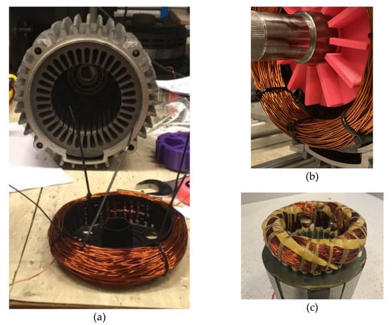
Figure 1.
(a) Coil for representation of the end winding and the stator of 4 kW benchmark induction motor; (b) assembled experimental model; (c) end winding of an electrical machine.

Table 1.
Electrical and geometric parameters of the coil, representing the end winding.
For the measurements, an aluminum alloy housing with a stator ferromagnetic core without windings from a 4 kW induction motor was used (Figure 1a). The coil was placed on the edge of the stator core, acting as an end winding, and it was firmly fixed using pre-shaped thermoplastic pieces, which slightly penetrated into the stator slots. The used thermoplastic is a good thermal insulator; hence, it did not affect the thermal processes of interest within the end-winding region and the steady-state temperature distribution. The coil was positioned at an offset distance from the stator core (Figure 1b) and the slots were closed with an insulation tape. In order to provide conditions, where the complete heat transfer takes place only in the end-winding region of the machine with the coil as the only heat source, the extensions of the winding, i.e., the active parts of the winding, placed into the stator slots, were not needed and were, thus, omitted. The coil configuration (Figure 1a) is not completely identical to the end winding of an electrical machine (Figure 1c), due to the lack of winding extensions going into the stator slots. However, such a coil configuration was necessary in order to achieve the controlled environment regarding the heat production and flow, i.e., to direct the heat toward the end-winding air region, and not into the active part of the machine (stator).
In a fully assembled electrical machine configuration, the winding extensions reduce the air motion in the space between the stator core edge and the end winding. Hence, varying the offset distance of the coil and placing it closer to the stator core surface allow reducing the cross-sectional area for the air flow in order to correspond to the real behavior of an electric machine. The distance from the stator core surface varied between 5 and 6 mm due to the uneven distribution of the wire within the coil bundle. The ends of the coil were pulled out from the end-winding region through a small opening in the housing and connected to the DC power supply. Insulation tape was placed on the edge of the stator core in order to avoid damage on the wire insulation varnish during the assembly process, to establish thermal insulation toward the stator core, and to avoid short-circuit and ground faults. The measurements in the region of interest were performed in the controlled environment, with the coil as the only heat source and convection as the only active heat transfer mechanism in the end-winding region, i.e., between the coil and the machine housing.
The constructed test rig consisted of a completely enclosed motor housing with the coil inside (experimental model), which was positioned and fixed on a measuring slot aluminum extrusion profile. The profile was placed on top of the laboratory table and it was well-attached to it (Figure 2a). The rotation of the shaft was provided by an induction drive motor, controlled with the variable-speed inverter with a rated power of 7.5 kW. The rotating shaft of the experimental model and the rotor of the drive motor were mechanically coupled via a torque sensor with a capacity of 10 Nm (Figure 2b). Due to the airflow, caused by the drive motor (TEFC—Totally Enclosed Fan Cooled type), an additional cardboard barrier had to be placed in-between in order to block the air flow along the shaft axis, which would have affected the thermal conditions and measurements. For the purpose of studying the blade configuration influence on the air flow in the end-winding region, different plastic (PLA—Poly Lactic Acid thermoplastic polymer) ventilation fans with blades were constructed and 3D-printed (Figure 3a).
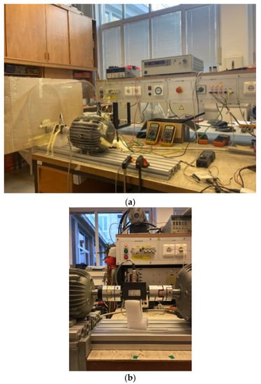
Figure 2.
(a) Experimental setup configuration; (b) mechanical coupling between the drive motor and experimental model.
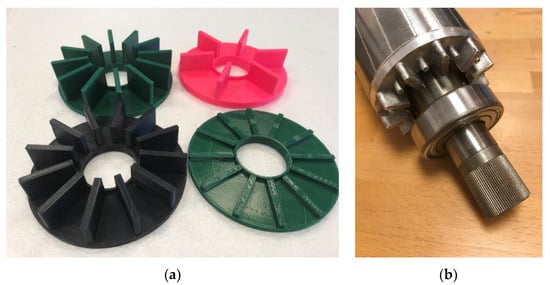
Figure 3.
(a) Three-dimensionally printed ventilation fans with different blade configurations; (b) die casted blades as an integral part of the rotor end ring of an induction machine.
Ventilation fans with various numbers of blades and heights were created, as shown in Table 2, in order to determine their impact on the heat exchange processes and to establish a relationship between the geometrical properties of the fan and the HTC. The ventilation fans were glued on the shaft to account for the centrifugal and torsional forces. They were positioned in such way to resemble the axial position of the real blades in electrical machines. In an induction machine, the blades are integral part of the rotor, i.e., they are manufactured in the squirrel-cage die-casting process (Figure 3b). For the permanent-magnet machines, the blades are attached as an additional component to the rotor, e.g., on the rotor balancing ring. Regardless of the production method of the blades, the air motion in the end-winding region depends only on the geometry of blades and the rotor rotational speed. Fans with additional features, such as curved blades or closure on both sides, should be analyzed with additional measurements and CFD calculations to obtain more accurate results.
Table 2.
Ventilation fans geometry.
Different heat power values do not affect the HTC, as the temperature difference changes proportionally with the heat flux as per Equation (4); thus, the only limitation when choosing heat power range values (10 W to 50 W) was the maximum allowed temperature for the insulation class of the copper wire and the glass-transition temperature of the 3D-printed PLA ventilation fans.
The purpose of the measurements was to determine the values of the steady-state temperatures and to obtain the temperature distribution in the experimental model for various independent variables, such as different rotational speeds ranging from 0 to 3000 min−1 and different fan configurations mounted on the shaft. During each experiment, several parameters were monitored and measured, i.e., electrical power supplied to the coil, temperatures at different spots, air velocity in the end-winding region, torque, and rotation speed. Temperatures were measured with type K-thermocouple sensors placed at different positions inside and outside the experimental model in order to obtain a more precise temperature distribution for the calibration of the thermal CFD model. Overall, 14 thermocouples were used for measuring. The arrangement of the thermocouple sensors is shown in Table 3 and their exact positions are shown in Figure 4.
Table 3.
Thermocouple sensors arrangement in the experimental model.
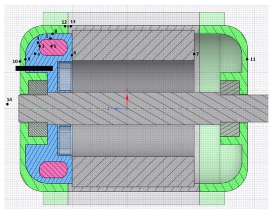
Figure 4.
Position of the thermocouple sensors for measuring temperatures. The black rectangle represents the position of the anemometer.
The air velocity in the end-winding region was measured with an anemometer with a maximum capacity of 20 m/s, which was placed inside the housing of the experimental model through a hole in the end cap (Figure 4), corresponding to its diameter and size. At the beginning of each measurement, the position and depth penetration of the anemometer was varied, combined with the rotation around its axis and the adjustment of the angle between the anemometer and end cap, in order to reach the maximum air velocity, i.e., to align the anemometer with the air flow.
2.3. Description of the CFD Model
The 3D CFD numerical model was built according to the dimensions of the experimental model components using the Ansys Fluent 19.3R software package. The geometry of the 3D model and ventilation fan model is shown in Figure 5a,b, respectively. The blades of the ventilation fan stretch from the shaft to the outer radius of the fan , which is equal to the outer rotor radius. The shaft radius is related to the outer rotor radius (Table 4 and Figure 5) according to the standard IEC 60072 (Rotating electrical machines—Dimensions and output series). In order to reduce computational time, the coil representing the end winding was simplified and modeled with a toroid. The axial length of the stator core in the model was shortened (dimension in Figure 6 and Table 4), as it had negligible effect on the thermal behavior in the end-winding region due to thermal insulation and low thermal conductivity in the axial direction (Table 5).
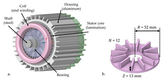
Figure 5.
(a) 3D geometric model; (b) ventilation fan model (12 blades, 13 mm high).
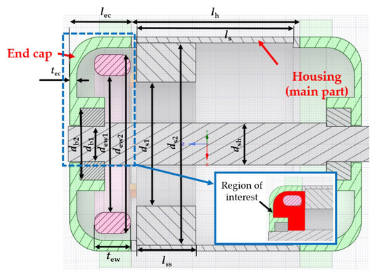
Figure 6.
Cross-sectional view of the CFD model with marked geometry parameters.
Table 5.
The material properties of the modelled components.
Figure 6 shows the cross-sectional view of the CFD model with the geometric parameters explained in Table 4. The region of interest, where the physical phenomena were analyzed in detail, is colored in red (zoomed area in Figure 6). The material properties assigned to the modeled components are given in Table 5. The thermal conductivities of the end winding and stator core are anisotropic; thus, there are three different values given in Table 5, referring to the thermal conductivity in radial, circumferential, and axial directions (, , ).
The accuracy of the CFD numerical simulations depends on the physical properties of the model; thus, the mesh density was manually adjusted for each region. A fine mesh must be used for the contact area between the solid components (e.g., coil and end cap) and the air in the end-winding region (fluid) in order to accurately model the air velocity and the temperature distribution. For this purpose, 5 inflation layers were added to the mesh at the boundaries of the air domain (Figure 7a). Solid components with good thermal conductivity (metals) can have larger elements, i.e., tetrahedron cells, while smaller cells have to be used for the air domains. The maximum cell size for the mesh of the solid objects was set to 9 mm. The cell sizes in the moving and stationary air domain were set to 1 mm and 2 mm, respectively. The total number of elements in the CFD model was 5.3 million, resulting in an average computational time of approximately 14 h per one CFD simulation. A result, showing the air velocity streamlines in the end-winding region, is presented in Figure 7b, and the temperature distribution in the region of interest is shown in Figure 7c.
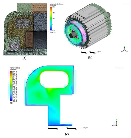
Figure 7.
CFD model cross-sectional view: (a) generated mesh; (b) air velocity distribution in the end-winding region; (c) temperature distribution in the end-winding region.
For a model containing rotating parts (e.g., ventilation fan), two different solving methods can be used, i.e., Moving Reference Frame (MRF) or Sliding Mesh. In the latter, the separate zones move relative to each other; thus, this method is appropriate for solving transient models. It is more accurate than the MRF method, but the computation time significantly increases. On the other hand, the MRF method is a steady-state approximation in which different rotational speeds can be set for individual cell zones. Instead of modeling the whole fan in the investigated model as an individual zone, only its walls, i.e., boundary end surfaces, are modeled as a part of an air domain that enclosures the fan and its immediate surrounding. The angular velocity of the fan was assigned to this moving air domain by using the MRF method. For the air flow outside the fan region, a stationary frame was generated.
The commercial software for CFD simulations Ansys Fluent, which was used in this study, offers different numerical approaches to solve the turbulences resulting from the rotating masses. The most often used approach is the Reynolds-Averaged Navier–Stokes (RANS) turbulent model, based on 2-transport equations. The most typical RANS models are k-ε and k-ω. The k-ε model is often used for flow calculations and heat transfer simulations due to reasonable accuracy for a wide range of turbulent flows, but it is not suitable nor accurate for flows that separate from the smooth surfaces. For such flows, it is more appropriate to use the k-ω model. However, the main drawback of the k-ω model is its sensitivity to freestream. The combination of k-ε and k-ω is the Shear Stress Transport (SST k-ω) model. It is not freestream-sensible and it is able to accurately compute the flow separation from smooth walls, which makes it an appropriate model for most flows. The SST k-ω model was chosen for all CFD calculations, presented in the paper.
All CFD simulations were run at the Laboratory of Electrical Machines, Faculty of Electrical Engineering, University of Ljubljana, on the workstation platform computer HPE Apollo r2800 Gen10 24SFF CTO Chassis with an HPE XL1x0r Gen10 Intel Xeon-Gold 6130 (2.1 GHz 16-core 125 W) processor with eight HPE 32 GB (1 × 32 GB) Dual Rank x4 DDR4-2666 units, resulting in 256 GB of RAM.
In the CFD model, presented in this study, the coil was geometrically simplified and it has the shape of a smooth toroid. In reality, the end winding is a bundle of wire with a non-smooth surface. However, the exact modeling of all end-winding details and its surface would have been extremely difficult, and it would have taken enormous computational resources. In order to improve the accuracy of the CFD model, the smooth surface of the toroid was altered by implementing a roughness height parameter ranging from 0 (zero roughness height assuming a smooth coil) to 1.3 mm (non-smooth coil), which corresponded to the wire diameter increase ranging from 0 to 125% (the wire diameter equals 1.05 mm). The difference between the numerically and experimentally determined HTC was assessed for the whole range of the introduced roughness parameters ranging from 0 mm to 1.3 mm. As per Table 6, where only the limit values’ roughness height parameters are given, the difference between the experimental and numerical HTC values decreases as the roughness height increases. The roughness height in the CFD model was selected at 1.3 mm (i.e., 125% of the wire diameter, thus representing a more realistic surface of the end-winding model), where the absolute difference between the HTC obtained by the experimental measurements and the 3D CFD simulations was smallest (Table 6). A further increase in the roughness height above 1.3 mm did not contribute to the reduction in the absolute difference between experimental and CFD results. Moreover, an additional increase in the roughness height above 1.3 mm would have increased the surface and improved the cooling effects, and the difference between the measured and calculated heat transfer coefficient would have been positive, meaning an increased value of the CFD calculated HTC with respect to the measured one.
Table 6.
Comparison of HTC values, obtained by CFD simulations, for different values of roughness height ( = 12, = 3000 min−1).
3. Results and Discussion
3.1. Validation of the CFD Model
In order to validate the CFD model, the comparison of temperature distribution was made. In Figure 8, the measured and calculated temperatures are shown for the ventilation fan with = 6 blades with a = 18 mm height at three different rotational speeds. Figure 9 shows the temperature distribution for the configuration = 12 and = 13 mm. Matching of the temperatures serves as a proof of correct behavior of the CFD model. A complete set of validation bar charts can be found in the Supplementary Material to the paper.
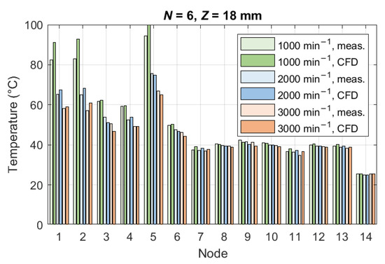
Figure 8.
Temperature distribution for = 6 and = 18 mm at different speeds.
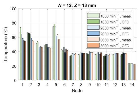
Figure 9.
Temperature distribution for = 12 and = 13 mm at different speeds.
In Figure 10, the HTC relation to the rotational speed , , is shown for six different blade configurations, i.e., = {3, 6, 12} at = 18 mm and = {3 mm, 13 mm, 23 mm} at = 12, with all numerical values collected in Table 7 (in the Section 3.3 Discussion). Good matching of the measurement and CFD results in all graphs is a proof of a well-calibrated CFD model. Thus, the CFD model was used for all further investigations regarding the convective heat transfer in the end-winding region.
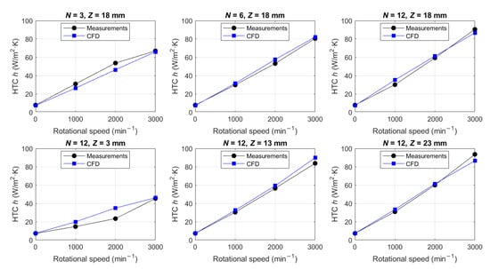
Figure 10.
HTC dependence on rotational speed . Comparison between CFD values and experimental measurement results.
3.2. Derivation of the Generalized Analytical Model
The curves in Figure 10 indicate that the HTC does not depend solely on the rotational speed, but also on the ventilation fan geometry, i.e., the blade configuration. The geometric parameters of the blades have a combined effect on the HTC in the end-winding region of rotating electrical machines. The studies in the domain of heat transfer analysis consider the HTC solely as a function of the air velocity in the end-winding region [1,8,10,11,12,13,14]. Obtaining the air velocity value is impossible without the CFD calculations or measurements; thus, the link between the air velocity and the rotor rotational speed is still missing. In the literature, it is called “fanning factor”, and its value is usually only estimated as a rule of thumb. However, knowing the exact value of the fanning factor increases the reliability of thermal analyses, as the convective heat transfer mechanism is much more accurately described. The derivation of the fanning function, which is a step toward the creation of the generalized analytical model, is presented below.
The relationship between the HTC and air velocity, , is already established in the published literature and it is described by Equation (6a). It was confirmed also by the CFD results, where Figure 11. shows the in the end-winding region for variety of blade configurations.
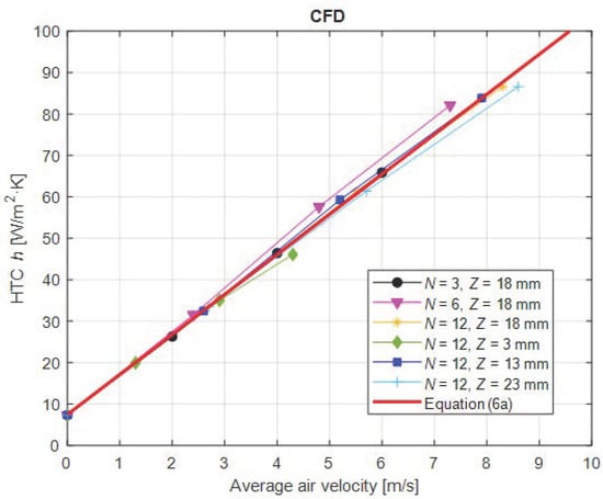
Figure 11.
HTC dependence on average air velocity in the end-winding region for variety of blade configurations. Values gained from CFD model.
The curves were obtained for all studied ventilation fans, with all of them having almost an identical slope, shown in Figure 11. According to that, Equation (6a) for describing the dependency in (W/m2K) was used:
where is average air velocity in the end-winding region in (m/s). Coefficients were obtained by a linear fit of the curves in Figure 11: , and . For low speeds, the coefficient usually ranges between 0.95 and 1 without having a significant influence on the behavior of the equation. The coefficient refers to the standstill rotor, when no forced convection is present, but only free air (natural) convection in the region of interest. It is in accordance with the published literature usually ranging between 5 and 30 W/m2·K [9] (p. 8) [12,23]. Equation (6a) has a similar form to the ones given in references [1,9,12], but with different values of the coefficients:
In order to find the correlation between the geometry of the ventilation fan and the HTC between the end winding and the surrounding air by analytical means, a coefficient , representing the fanning factor, is introduced as a ratio of the average air velocity and the peripheral rotational speed of the rotor, and , respectively:
The connection between rotor peripheral speed, , given in (m/s), and rotational speed, , given in (min−1), is calculated according to Equation (8):
where is the angular velocity (s−1), is the rotor rotational speed (min−1), and is the outer rotor radius (mm).
In this study, the fanning factor was analytically determined by using a product of three generalized logistic functions (Equation (10)). The logistic function, Equation (9), has been proven to be a useful mathematical tool for studying and forecasting behavior of different scientific phenomena [24]:
where is the maximum value of the curve, is the logistic growth rate, is the Euler’s number, is the value of the curve, and is an independent variable (real number).
The logistic function in Equation (9) allows for identification of parameters for the quantitative analyses, such as saturation level, midpoint, and growth rate. Therefore, it was selected for the description of the fanning factor , treated as a fanning function further on, as the HTC dependence and both exhibit an exponential growth tendency followed by a saturation, as per Figure 8 and Figure 9. Further on, the CFD results also indicate the dependence of the HTC on the outer rotor radius (see Table 7, Table 8 and Table 9).
The final form of the equation for the calculation of fanning function (Equation (10)), defined as a function of the number of blades , blade height (in (mm)), and rotor radius (in (mm)), was derived from the CFD simulation results. The equation is valid for , , and , and is also reasonable out of these limits (extrapolation of the function):
The coefficients in Equation (10) were obtained by using nlinfit nonlinear regression in Matlab software with zero vector for the initial coefficient values. The coefficient is the product of three logistic function maximum values ().
Figure 12 and Figure 13 show the fanning function vs. blade height ( = 12) and the number of blades ( = 18 mm), respectively, at a rotor rotational speed of 3000 min−1. In both graphs, the analytically calculated values by Equation (10), illustrated with red lines, as well as CFD results, marked with blue points, are shown for three different radii (26 mm, 52 mm, and 78 mm). Both figures visualize the correct behavior of the analytical equation (Equation (10)), also with slight extrapolation outside the specified range.
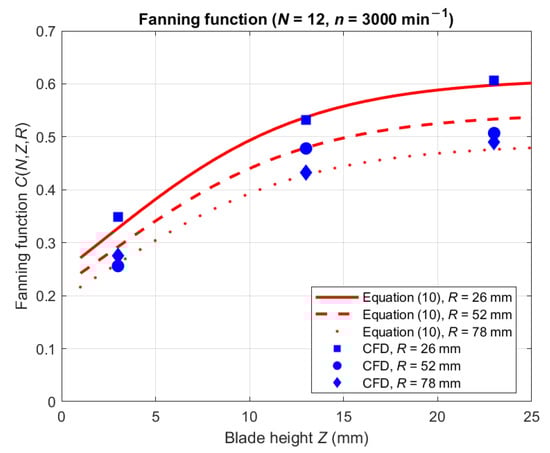
Figure 12.
Fanning function vs. the blades height ( = 12) at = 3000 min−1.
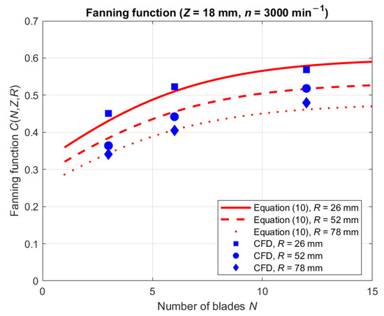
Figure 13.
Fanning function vs. the number of blades ( = 18 mm) at = 3000 min−1.
By knowing the fanning function , the average air velocity in the end-winding region is defined in accordance with (7):
Equation (11) is then included in (6a), which represents the conventional approach for calculating the HTC, giving (12):
Finally, by combining (8), (10), and (12), the analytical model for improved calculation of the HTC in the end-winding region of electrical machines in relation to the blades geometry ( in (W/m2K)) is derived (13):
where:
- is the rotational speed (min−1);
- is the number of blades;
- is the outer rotor diameter (mm);
- Z is the blade height (mm).
3.3. Discussion
Table 7 shows a comparison between the HTC, obtained from measurements and the CFD model, as well as calculated with the novel approach, given by Equation (13), and three reference equations, given by Equations (6b)–(6d), all of them for different blade geometries and rotational speeds. The column containing the average air speed in the end-winding region, , is added for the determination of HTC values according to Equations (6b)–(6d). The comparison of the HTC values is graphically presented in Figure 14. Table 8 and Table 9 show the difference between the novel approach and reference equations for calculating the HTC compared to CFD simulation results, for = 26 mm and = 78 mm, respectively. It can be seen that using the novel approach significantly increases the accuracy of the calculation for a wide range of ventilation fan geometries. The accuracy increase is reflected in the correct slope as well as correct values (Figure 14), obtained by the novel approach.
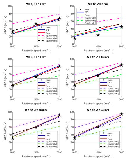
Figure 14.
Graphical representation of the difference between the results according to Table 7.
Table 7.
Comparison between novel approach and reference equations for calculating HTC compared to measurements and CFD simulation results ( = 52 mm).
Table 7.
Comparison between novel approach and reference equations for calculating HTC compared to measurements and CFD simulation results ( = 52 mm).
(mm) | (min−1) | (W/m2·K) | (6b) (W/m2·K) | (6c) (W/m2·K) | (6d) (W/m2·K) | ||||
|---|---|---|---|---|---|---|---|---|---|
| 3 | 18 | 1000 | 30.9 | 26.3 | 1.96 | 27.7 | 53.6 | 27.9 | 35.5 |
| 2000 | 53.7 | 46.4 | 3.98 | 48.0 | 66.2 | 39.0 | 50.3 | ||
| 3000 | 67.0 | 65.9 | 6.00 | 68.2 | 78.7 | 49.6 | 62.4 | ||
| 6 | 1000 | 29.8 | 31.5 | 2.39 | 31.4 | 56.3 | 30.4 | 39.0 | |
| 2000 | 53.2 | 57.6 | 4.81 | 55.4 | 71.3 | 43.4 | 55.5 | ||
| 3000 | 80.5 | 82.1 | 7.28 | 79.4 | 86.7 | 56.0 | 69.2 | ||
| 12 | 1000 | 30.1 | 35.2 | 2.88 | 34.7 | 59.3 | 33.1 | 42.7 | |
| 2000 | 59.3 | 61.3 | 5.58 | 61.9 | 76.1 | 47.4 | 60.1 | ||
| 3000 | 90.5 | 86.6 | 8.39 | 89.1 | 93.6 | 61.6 | 74.8 | ||
| 12 | 3 | 1000 | 14.7 | 19.9 | 1.32 | 22.9 | 49.6 | 24.2 | 29.6 |
| 2000 | 23.4 | 35 | 2.86 | 38.2 | 59.2 | 33.0 | 42.6 | ||
| 3000 | 45.4 | 46.1 | 4.29 | 53.6 | 68.1 | 40.7 | 52.3 | ||
| 13 | 1000 | 30.4 | 32.5 | 2.58 | 32.7 | 57.4 | 31.4 | 40.5 | |
| 2000 | 56.5 | 59.3 | 5.22 | 57.9 | 73.9 | 45.5 | 58.0 | ||
| 3000 | 83.8 | 83.9 | 7.88 | 83.2 | 90.4 | 59.0 | 72.3 | ||
| 23 | 1000 | 30.9 | 33.4 | 2.69 | 35.5 | 58.1 | 32.0 | 41.3 | |
| 2000 | 60.0 | 61.4 | 5.43 | 63.6 | 75.2 | 46.6 | 59.2 | ||
| 3000 | 93.6 | 86.6 | 8.65 | 91.7 | 95.2 | 62.8 | 76.0 |
Table 8.
Comparison between novel approach and reference equations for calculating HTC compared to CFD simulation results (R = 26 mm).
Table 8.
Comparison between novel approach and reference equations for calculating HTC compared to CFD simulation results (R = 26 mm).
| Z (mm) | n (min−1) | hCFD (W/m2·K) | (W/m2·K) | (6b) (W/m2·K) | (6c) (W/m2·K) | (6d) (W/m2·K) | ||
|---|---|---|---|---|---|---|---|---|
| 3 | 18 | 1000 | 16.8 | 1.20 | 18.8 | 48.9 | 23.5 | 28.4 |
| 2000 | 28.2 | 2.46 | 30.1 | 56.7 | 30.8 | 39.6 | ||
| 3000 | 38.3 | 3.75 | 41.5 | 64.7 | 37.8 | 48.8 | ||
| 6 | 1000 | 17.8 | 1.55 | 20.9 | 51.0 | 25.6 | 31.8 | |
| 2000 | 31.4 | 3.08 | 34.3 | 60.6 | 34.2 | 44.2 | ||
| 3000 | 46.1 | 4.67 | 47.7 | 70.4 | 42.7 | 54.7 | ||
| 12 | 1000 | 17.8 | 1.55 | 22.7 | 51.0 | 25.6 | 31.8 | |
| 2000 | 31.4 | 3.08 | 37.9 | 60.6 | 34.2 | 44.2 | ||
| 3000 | 46.1 | 4.67 | 53.2 | 70.4 | 42.7 | 54.7 | ||
| 12 | 3 | 1000 | 18.9 | 0.87 | 16.1 | 46.8 | 21.5 | 24.7 |
| 2000 | 29.7 | 1.95 | 24.7 | 53.5 | 27.9 | 35.4 | ||
| 3000 | 42.5 | 3.00 | 33.3 | 60.1 | 33.8 | 43.7 | ||
| 13 | 1000 | 17.7 | 1.43 | 21.6 | 50.3 | 24.9 | 30.7 | |
| 2000 | 34.1 | 2.93 | 35.7 | 59.6 | 33.3 | 43.1 | ||
| 3000 | 49.2 | 4.35 | 49.9 | 68.5 | 41.0 | 52.7 | ||
| 23 | 1000 | 18.4 | 1.65 | 23.2 | 51.7 | 26.2 | 32.7 | |
| 2000 | 34.2 | 3.30 | 38.9 | 61.9 | 35.4 | 45.8 | ||
| 3000 | 49.7 | 4.97 | 54.6 | 72.3 | 44.2 | 56.5 |
Table 9.
Comparison between novel approach and reference equations for calculating HTC compared to CFD simulation results (R = 78 mm).
Table 9.
Comparison between novel approach and reference equations for calculating HTC compared to CFD simulation results (R = 78 mm).
| Z (mm) | (min−1) | (W/m2·K) | (W/m2·K) | (6b) (W/m2·K) | (6c) (W/m2·K) | (6d) (W/m2·K) | ||
|---|---|---|---|---|---|---|---|---|
| 3 | 18 | 1000 | 28.8 | 2.73 | 34.6 | 58.4 | 32.3 | 41.6 |
| 2000 | 51.2 | 5.58 | 61.7 | 76.1 | 47.4 | 60.1 | ||
| 3000 | 72.8 | 8.52 | 88.8 | 94.4 | 62.2 | 75.4 | ||
| 6 | 1000 | 35.9 | 3.28 | 39.5 | 61.8 | 35.3 | 45.6 | |
| 2000 | 67.4 | 6.68 | 71.6 | 82.9 | 53.0 | 66.1 | ||
| 3000 | 93.3 | 9.95 | 103.7 | 103.3 | 69.2 | 82.1 | ||
| 12 | 1000 | 42.8 | 3.95 | 43.9 | 66.0 | 38.9 | 50.1 | |
| 2000 | 77.4 | 7.78 | 80.3 | 89.8 | 58.5 | 71.8 | ||
| 3000 | 108.7 | 11.66 | 116.7 | 113.9 | 77.4 | 89.7 | ||
| 12 | 3 | 1000 | 23.1 | 2.14 | 28.1 | 54.7 | 29.0 | 37.0 |
| 2000 | 44.5 | 4.55 | 48.7 | 69.7 | 42.1 | 53.9 | ||
| 3000 | 64.0 | 6.97 | 69.3 | 84.8 | 54.5 | 67.6 | ||
| 13 | 1000 | 38.8 | 3.52 | 41.3 | 63.3 | 36.6 | 47.3 | |
| 2000 | 70.6 | 7.12 | 75.0 | 85.7 | 55.2 | 68.4 | ||
| 3000 | 97.5 | 10.54 | 108.8 | 107.0 | 72.0 | 84.8 | ||
| 23 | 1000 | 44.5 | 4.09 | 45.1 | 66.8 | 39.6 | 51.1 | |
| 2000 | 82.2 | 8.27 | 82.6 | 92.8 | 61.0 | 74.2 | ||
| 3000 | 115.5 | 11.35 | 120.2 | 112.0 | 75.9 | 88.3 |
Figure 15 shows graphical representations of the calculated value of HTC according to Equation (13). Results for three different radii of the ventilation fans ( = {26, 52, 78} mm) are shown in rows, whereas the results for different speeds ( = {1000, 2000, 3000} min−1) are shown in columns (Figure 15). It can be seen in all graphs that increasing the number of blades above > 8 and blade height above > 15 mm does not increase the HTC significantly. Namely, a comparison of the HTC values at = 12 and = 25 mm with = 8 and = 15 mm (+50% increase of and +66.7% increase of ) shows a relative increase in HTC in the range between 9% and 14%, depending on the outer radius and rotational speed. Such information is essential, for example, for the concept design of the end-winding region ventilation system.
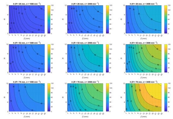
Figure 15.
Value of HTC h (in (W/m2K)), calculated by analytical model (13), for different rotor radii, rotational speeds, number of blades, and blade height.
4. Conclusions
A thorough analysis of the convective heat transfer in the end-winding region of an electrical machine from the stator end winding to the surrounding air was performed using a 3D CFD modeling approach that was successfully validated with the experimental measurements. The results, presented in this study, can be used for the heat transfer analysis of any electrical machine type with a distributed winding configuration on the stator side and having blades mounted on the rotor, which help improve the stator cooling performance.
Based on our experimental results, supported with the CFD modeling simulations, the analytical model for the calculation of the HTC was derived. The important advantage of the derived model is that it takes into account the realistic geometric properties of the ventilation fan, which are available already in the electrical machine design phase (outer rotor radius, number of blades, and blade height), and rotor rotational speed, without the need of knowing the average air speed. The air speed can be obtained only by CFD or measurements. The proposed analytical model can also be used for the thermal modeling of the already existing machine, e.g., included in the lumped-parameter thermal network, thus providing a useful tool to calculate the HTC in the low-speed region up to 3000 min−1, where the majority of electric machine overload operations occur. The equation is valid in the parameter ranges = [3, 12], = [3, 23] mm, and = [26, 78] mm, and is also reasonable out of these limits (extrapolation of the function). Our future research work will involve also the investigation of higher rotational speeds in order to verify the derived equation for the rotational speeds above 3000 min−1 in the regions of interest.
It should be emphasized that the direct connection between the HTC and rotational speed of the rotor represents a significant achievement, which will allow the study of ventilation fan concept designs in the early stage of the electric machine design process as well as an improved accuracy of HTC calculation, leading to more precise thermal modeling (e.g., with lumped-parameter thermal network) and allowing various rapid thermal optimizations without the need of computationally demanding CFD calculations.
Supplementary Materials
The following supporting information can be downloaded at: https://www.mdpi.com/article/10.3390/en16020930/s1, Validation of the CFD model.
Author Contributions
Conceptualization, M.V., S.L., D.M., and S.Č.; methodology, M.V., S.L., N.Š., D.M., and S.Č.; software, M.V.; validation, S.L. and N.Š.; formal analysis, M.V. and S.Č.; investigation, M.V., S.L., N.Š., and S.Č.; resources, D.M. and S.Č.; data curation, M.V., S.L., and N.Š.; writing—original draft preparation, S.L., N.Š., and S.Č.; writing—review and editing, M.V. and S.Č.; visualization, M.V., S.L., and N.Š.; supervision, D.M. and S.Č.; project administration, D.M.; funding acquisition, D.M. All authors have read and agreed to the published version of the manuscript.
Funding
This research has received funding from the European Union’s Horizon 2020 research and innovation program under grant agreement number 101006747.
Data Availability Statement
Not applicable.
Acknowledgments
The authors acknowledge the European Union for the Horizon 2020 research and innovation program under grant agreement number 101006747.
Conflicts of Interest
The authors declare no conflict of interest.
References
- Boglietti, A.; Cavagnino, A. Analysis of the endwinding cooling effects in TEFC induction motors. IEEE Trans. Ind. Appl. 2007, 43, 1214–1222. [Google Scholar] [CrossRef]
- Previati, G.; Mastinu, G.; Gobbi, M. Thermal Management of Electrified Vehicles—A Review. Energies 2022, 15, 1326. [Google Scholar] [CrossRef]
- Gronwald, P.-O.; Kern, T.A. Traction Motor Cooling Systems: A Literature Review and Comparative Study. IEEE Trans. Transp. Electrif. 2021, 7, 2892–2913. [Google Scholar] [CrossRef]
- Lehmann, R.; Künzler, M.; Moullion, M.; Gauterin, F. Comparison of Commonly Used Cooling Concepts for Electrical Machines in Automotive Applications. Machines 2022, 10, 442. [Google Scholar] [CrossRef]
- La Rocca, S.; Pickering, S.J.; Eastwick, C.N.; Gerada, C.; Rönnberg, K. Fluid flow and heat transfer analysis of TEFC machine end regions using more realistic end-winding geometry. In Proceedings of the 9th International Conference on Power Electronics, Machines and Drives (PEMD 2018), Liverpool, UK, 17–19 April 2019; Volume 2019, pp. 3831–3835. [Google Scholar]
- Im, S.; Gu, B. Interturn Fault Tolerant Drive Method by Limiting Copper Loss of Interior Permanent Magnet. IEEE Trans. Ind. Electron. 2020, 67, 7973–7981. [Google Scholar] [CrossRef]
- Zoeller, C.; Vogelsberger, M.A.; Fasching, R.; Grubelnik, W.; Wolbank, T.M. Evaluation and Current-Response-Based Identification of Insulation Degradation for High Utilized Electrical Machines in Railway Application. IEEE Trans. Ind. Appl. 2017, 53, 2679–2689. [Google Scholar] [CrossRef]
- Staton, D.A.; Popescu, M.; Hawkins, D.; Boglietti, A.; Cavagnino, A. Influence of Different End Region Cooling Arrangements on End-Winding Heat Transfer Coefficients in Electrical Machines. In Proceedings of the 2010 IEEE Energy Conversion Congress and Exposition, Atlanta, GA, USA, 12–16 September 2010; IEEE: Atlanta, GA, USA; pp. 1298–1305. [Google Scholar]
- Ahmed, F.; Kar, N.C. Analysis of End-Winding Thermal Effects in a Totally Enclosed Fan-Cooled Induction Motor With a Die Cast Copper Rotor. IEEE Trans. Ind. Appl. 2017, 53, 3098–3109. [Google Scholar] [CrossRef]
- Nachouane, A.B.; Abdelli, A.; Friedrich, G.; Vivier, S. Numerical Study of Convective Heat Transfer in the End Regions of a Totally Enclosed Permanent Magnet Synchronous Machine. IEEE Trans. Ind. Appl. 2017, 53, 3538–3547. [Google Scholar] [CrossRef]
- Basso, G.L.; Goss, J.; Staton, D. Improved thermal model for predicting end-windings heat transfer. In Proceedings of the 2017 IEEE Energy Conversion Congress and Exposition (ECCE), Cincinnati, OH, USA, 1–5 October 2017; pp. 4650–4657. [Google Scholar]
- Groschup, B.; Nell, M.; Pauli, F.; Hameyer, K. Characteristic Thermal Parameters in Electric Motors: Comparison Between Induction- and Permanent Magnet Excited Machine. IEEE Trans. Energy Convers. 2021, 36, 2239–2248. [Google Scholar] [CrossRef]
- Tovar-Barranco, A.; López-de-Heredia, A.; Villar, I.; Briz, F. Modeling of End-Space Convection Heat-Transfer for Internal and External Rotor PMSMs With Fractional-Slot Concentrated Windings. IEEE Trans. Ind. Electron. 2021, 68, 1928–1937. [Google Scholar] [CrossRef]
- Veg, L.; Laksar, J. Impact of Thermal Conductivity in Axial Direction on the Overall Thermal Model of High-Speed Synchronous Motor. In Proceedings of the 2018 XIII International Conference on Electrical Machines (ICEM), Alexandroupoli, Greece, 3–6 September 2018; IEEE: Alexandroupoli, Greece; pp. 1234–1239. [Google Scholar]
- Mellor, P.H.; Roberts, D.; Turner, D.R. Lumped parameter thermal model for electrical machines of TEFC design. IEEE Proc. B Electr. Power Appl. 1991, 138, 205–218. [Google Scholar] [CrossRef]
- Madonna, V.; Walker, A.; Giangrande, P.; Serra, G.; Gerada, C.; Galea, M. Improved Thermal Management and Analysis for Stator End-Windings of Electrical Machines. IEEE Trans. Ind. Electron. 2019, 66, 5057–5069. [Google Scholar] [CrossRef]
- Jeong, M.; Yun, J.; Park, Y.; Lee, S.B.; Gyftakis, K. Off-line Flux Injection Test Probe for Screening Defective Rotors in Squirrel Cage Induction Machines. In Proceedings of the 2017 IEEE 11th International Symposium on Diagnostics for Electrical Machines, Power Electronics and Drives (SDEMPED), Tinos, Greece, 29 August 2017–1 September 2017; IEEE: Tinos, Greece. [Google Scholar]
- Jungreuthmayer, C.; Bäuml, T.; Winter, O.; Ganchev, M.; Kapeller, H.; Haumer, A.; Kral, C. A Detailed Heat and Fluid Flow Analysis of an Internal Permanent Magnet Synchronous Machine by Means of Computational Fluid Dynamics. IEEE Trans. Ind. Electron. 2012, 59, 4568–4578. [Google Scholar] [CrossRef]
- Čorović, S.; Šutar, N.; Miljavec, D. Modeling of Thermal Effects in Induction Machines due to the Stator End-Windings. In Proceedings of the 2020 19th International Conference on Mechatronics—Mechatronika, ME 2020, Prague, Czech Republic, 2–4 December 2020. [Google Scholar]
- Comsol, “Heat Transfer: Conservation of Energy”. Available online: https://www.comsol.com/multiphysics/heat-transfer-conservation-of-energy#ref (accessed on 24 October 2022).
- Arbab, N.; Wang, W.; Lin, C.; Hearron, J.; Fahimi, B. Thermal Modeling and Analysis of a Double-Stator Switched Reluctance Motor. IEEE Trans. Energy Convers. 2015, 30, 1209–1217. [Google Scholar] [CrossRef]
- Bergman, T.L.; Lavine, A.S.; Incropera, F.O.; Dewitt, D.P. Fundamentals of Heat and Mass Transfer, 7th ed.; John Wiley and Sons: Hoboken, NJ, USA, 2011. [Google Scholar]
- Gai, Y.; Kimiabeigi, M.; Chong, Y.C.; Widmer, J.D.; Deng, X.; Popescu, M.; Goss, J.; Staton, D.A.; Steven, A. Cooling of Automotive Traction Motors: Schemes, Examples, and Computation Methods. IEEE Trans. Ind. Electron. 2019, 66, 1681–1692. [Google Scholar] [CrossRef]
- Kucharavy, D.; De Guio, R. Application of Logistic Growth Curve. Procedia Eng. 2015, 131, 280–290. [Google Scholar] [CrossRef]


Disclaimer/Publisher’s Note: The statements, opinions and data contained in all publications are solely those of the individual author(s) and contributor(s) and not of MDPI and/or the editor(s). MDPI and/or the editor(s) disclaim responsibility for any injury to people or property resulting from any ideas, methods, instructions or products referred to in the content. |
© 2023 by the authors. Licensee MDPI, Basel, Switzerland. This article is an open access article distributed under the terms and conditions of the Creative Commons Attribution (CC BY) license (https://creativecommons.org/licenses/by/4.0/).