Article

The Influence of Noise Level on the Value of Uncertainty in a Measurement System Containing an Analog-to-Digital Converter

by
Eligiusz Pawłowski
1,
Anna Szlachta
2,* and
Przemysław Otomański
3
1
Department of Automation and Metrology, Faculty of Electrical Engineering and Computer Science, Lublin University of Technology, Nadbystrzycka Street 38A, 20-618 Lublin, Poland
2
Department of Metrology and Measurement Systems, Faculty of Electrical and Computer Engineering, Rzeszow University of Technology, W. Pola Street 2, 35-959 Rzeszow, Poland
3
Institute of Electrical Engineering and Electronics, Faculty of Control, Robotics and Electrical Engineering, Poznan University of Technology, Piotrowo Street 3A, 60-965 Poznan, Poland
*
Author to whom correspondence should be addressed.
Energies 2023, 16(3), 1060; https://doi.org/10.3390/en16031060
Submission received: 19 December 2022 / Revised: 13 January 2023 / Accepted: 15 January 2023 / Published: 18 January 2023

Abstract

:
For newly developed measuring systems, it is easy to estimate type-B uncertainties based on technical data from the measuring modules applied. However, it is difficult to estimate A-type uncertainties due to the unknown type and level of interferences infiltrating the measuring system. This is a particularly important problem for measurements carried out in the presence of typical of power grid disturbances. The aim of the research was to develop a method and a measurement stand for experimental assessment of uncertainties in a measuring system that makes use of data acquisition modules containing analog-to-digital converters (ADCs). The paper describes, in detail, the design of a completed test stand. It presents an original application in the LabVIEW environment, which enables testing the dependence of the uncertainties with the quantity of the measurements averaged in a series, for different kinds and levels of interferences infiltrating the measuring path. The results of tests for several popular measuring modules are presented. An analysis of the determined uncertainties was carried out in relation to the parameters of the tested measurement modules and for various levels of interferences. It is proved that an increase in the number of averaged measurements to approx. 100–200 always results in a decrease in uncertainty for each tested module and under all conditions. However, a further increase in the quantity of measurements, even up to 1000 averaged measurements, proved reasonable only for high-accuracy modules, in particular with a high level of interferences. An excessive increase in the quantity of averaged measurements proved a low effect for modules characterised by a low resolution and with a low level of interferences. The measurement results also proved that when estimated, uncertainties in the interference probability distribution are significant, especially if they deviate from normal distribution.

1. Introduction

Interference in the power grid can significantly affect the reliability of a measurement. For this reason, the topic is of interest to many authors. The article deals with the subject of measurements in the presence of disturbances in typical power grids. This has a significant impact on the accuracy of measurements, as well as on the correct assessment of power quality.

1.1. Motivations

The issue of the impact of electromagnetic interference, generated by alternating voltages, on the operation of selected measuring devices is addressed in many works. Publications [1,2,3] present the conditions that must be met to correctly to analyze the parameters that characterize the power grid.
Harmonic and interharmonic distortions, such as flicker, voltage dips, and so on, occur in power grids. These distortions cause a number of problems, both in these power grids and in the measurement systems that operate in the neighborhood [4].
In the present study, the authors focused on evaluating the impact of DC voltage interference on the operation of a measurement system containing an A/D converter.
Contemporary measuring systems are often built on the basis of computer data acquisition modules that contain analog-to-digital converters (ADCs).

1.2. State of the Art

In practice, a popular solution for such measurement systems is the use of virtual instruments, in particular implemented in the LabVIEW environment. The design and use of virtual instruments (VIs) is an important issue because VIs offer a unique feature that allows for customization of the instrument. The use of LabVIEW makes it possible to reduce the construction time of the measurement system, increase its reliability, and reduce design costs. This issue has been the subject of many publications [5,6,7,8,9,10,11]. The calculation of measurement uncertainty should be included in virtual instruments, but so far, no suitable algorithms have been developed that are part of commercial measurement application development environments. For this reason, the implementation of uncertainty calculation lies with the developers of virtual instruments. A correct application for uncertainty evaluation should have appropriate features that will enable the design of measurement systems, users who are not experts in metrology. The first step may be an application that allows for simulation studies with a properly developed virtual instrument [5]. The next step may be to use LABVIEW graphical software to simulate and measure various harmonics, noise, and impulse transients in sinusoidal voltage waveforms on the grid [6]. Better results can be achieved by replacing simulated signals with real signals from arbitrary generators [7]. In addition, the signals to be analyzed can be DC signals [5] or sinusoidal signals with various disturbances [6,8]. Distortion can be represented in the form of mathematical models, which can be used to analyze and measure parameters related to power quality, such as sag and swell, power frequency distortion, and harmonic distortion [8]. The best evaluation of the metrological properties of a measurement system can be obtained for signals recorded in an actual measurement system [9,10,11]. This draws attention to doubts about the reliability of the proposed methodology to represent the measurement result with its uncertainty based on the probabilistic Monte Carlo method [9]. A particular difficulty is the development of virtual instruments for the detection, analysis, and processing of current pulse signals in high-voltage measurement systems [10]. Other problems are encountered in the case of virtual instruments (VIs) for power quality monitoring, in which different types of windows are used: rectangular, Hanning, Blackman, etc. [11].
As presented, an important problem is the determination of uncertainty, according to documents [12,13,14], of measurements made in measurement systems and virtual instruments, especially under industrial conditions when there are disturbances [15,16,17].
All uncertainty calculations in the presented work were performed in accordance with the cited guides, primarily: Evaluation of measurement data—Guide to the expression of uncertainty in measurement, JCGM 100:2008 [12]. Type A uncertainties are due to disturbances in the measurement system. Type-B uncertainties, on the other hand, result from the performance of the measurement instrument. The expanded uncertainty U is the result of the combination of these two uncertainties and is, therefore, related to the measurement results. Therefore, the expanded uncertainty U cannot be attributed to either the measurement system or the measuring instrument.
The process of determining the expanded uncertainty was undertaken in the paper [18]. Here, a method is presented for estimating the uncertainty of the measurement result for both mutually uncorrelated and correlated input quantities. The study involved measurements of small resistances using an indirect method. Another example of determining uncertainty in a strain-measurement process is presented in [19]. In this case, a non-contact measurement method using optoelectronic elements was used.
When designing a new measuring system, it is relatively easy to predict the level of expected type-B uncertainties, by calculating them according to known rules [12,13] based on the available technical data of the applied measuring modules [20,21,22,23]. It is much more difficult to estimate the expected type-A uncertainty values and, thereby, it is difficult to determine the expanded uncertainty of the measurement result. This requires a series of single measurements and their appropriate compilation using statistical methods [12]. Repeating measurements multiple times makes the tests being carried out very time consuming. Nevertheless, such an approach ensures that the measurements carried out are objective and reliable and make it possible to formulate unambiguous conclusions.
It should also be noted that there may be systematic errors in measurement systems and, in this case, these should be corrected before the uncertainty can be estimated to the best of our knowledge. Disturbances that occur in the considered measurement system are random errors, not systematic errors.
In order to accomplish the intended aim, first of all, an optimum quantity of averaged measurements in the series must be established, which is difficult without prior knowledge of the level and type of the expected interferences in the measuring path.
In summary, the authors of the cited works describe virtual instruments that allow for simulation studies [5,6,8], in a real measurement system [7,10,11], or include both [9]. Simulation studies usually use analytical [5,6,8,9] or Monte Carlo [5,9] methods. Tests using real measurement data use measurement modules that measure signals with precisely known parameters obtained from programmable arbitrary generators [7,10] or tests are performed in a measurement system in the presence of real disturbances [9,11]. Usually, measurements in the real system are made with only one type of measurement module and only a few authors compare different measurement modules [7]. Therefore, it is difficult to assess the relationship between the parameters of the measurement module used and the measurement uncertainties obtained in the system. There is also a lack of work that analyzes, in a real system, the effect of the level and type of interference on measurement uncertainties, especially the effect on type-A uncertainties. According to Guide [12], Type-A uncertainties are determined by statistical methods based on a series of measurement results. Therefore, the appropriate selection of the number of measurements in a series is an important issue, especially in a real measurement system where the level and type of interference are not known in advance. In addition, the interference parameters change over the course of the measurements. These important issues have not yet been addressed in the available works under consideration.

1.3. Contributions

The paper presents a method of assessment of measurement uncertainties, which makes it possible to select an appropriate quantity of averaged measurements in relation to the parameters of the ADC applied in the measuring module and the type of interferences.
Section 2.1 presents a developed and constructed measuring position, which enables performance of tests for any measuring modules supported from the LabVIEW environment level. Section 2.2 describes an application created in the LabVIEW environment, which enables testing uncertainties depending on the quantity of the measurements averaged in a series, for different kinds and levels of interferences infiltrating the measuring path. This section presents equations that allow for calculation of uncertainties, taking into account approximate methods, which are often employed in measurement practice.
Section 3 contains the results of the experimental tests in a graphical and numerical form, for four popular measuring modules.
Section 4 and Section 5 include discussion of the obtained results, conclusions, and a summary of the obtained test results.

2. Materials and Methods

The constructed measurement stand is composed of a measuring instrument and a computer with an application that controls the measurements, which was created in the LabVIEW environment. The stand enables tests for any measuring modules equipped with a USB interface and having appropriate software drivers running in the LabVIEW environment. As part of the research, example tests were carried out for four measuring modules shown in Figure 1.
All modules were tested in a range of ±10 V in the differential configuration of the inputs. The technical data of the modules, which are necessary for determining the measurement uncertainties, are presented in Table 1.
To calculate the type-B uncertainty, according to Guide [12], first, calculate the maximum permissible error Δmpe of the measurement module. This error was calculated according to the manufacturer’s documentation [20,21,22,23] taking into account: multiplicative component—Gain Error; additive component—Offset Error; and noise component—Random Error. The Limit Error value was provided by the manufacturer as an example value for the full range 10 V and averaging 10,000 points. Therefore, it is not useful to calculate the uncertainty of the presented measurements.
Modules USB-6001 [20] and USB-6008 [21] are offered for education purposes, have a low resolution, 12 up to 14 bits, and relatively high maximum permissible errors. The manufacturer provides the technical data of these modules in a simplified manner and omits certain error components. Modules USB-9215 [20] and USB-6341 [23] for professional applications have a higher resolution of 16 bits and relatively low maximum permissible errors. Further, the technical data of these modules contain more detailed information.

2.1. Measurement System for Evaluating Uncertainty of Measurement Modules

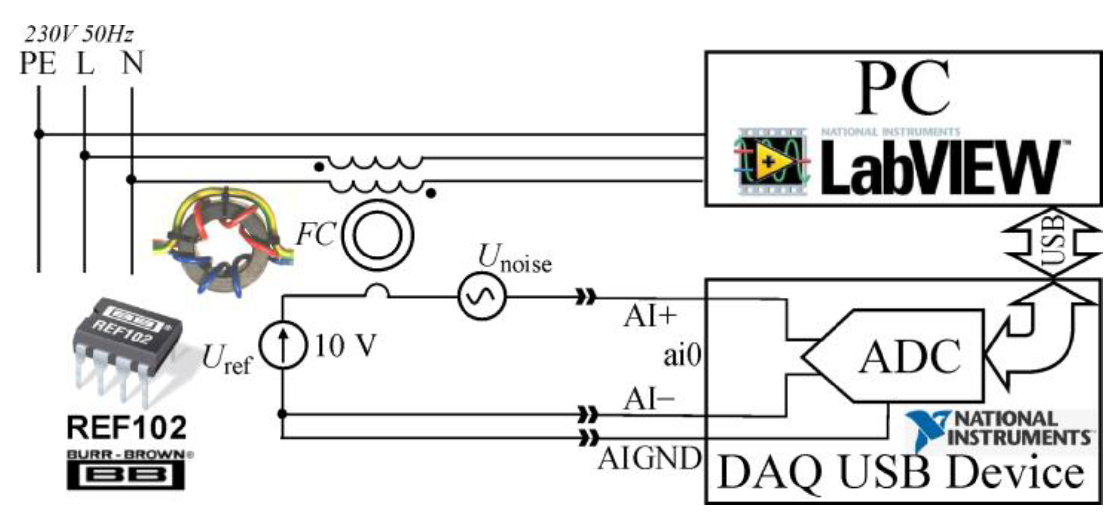
A diagram of the constructed measuring system is presented in Figure 2. This is a modified version of the system described in the previous papers by the authors of [16]. Following a preliminary analysis [16,24], a precise high-stability source of reference voltage Uref = 10 V of REF 102 type was applied [25], the most important parameters of which are presented in Table 2.
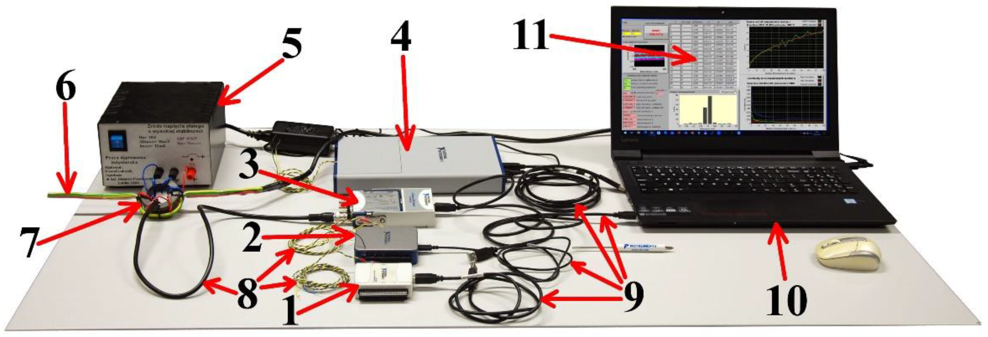
The tested measuring device is connected to a personal computer (PC) via a USB interface. The measurements were carried out in differential mode in the ai0 channel, but it is possible to choose a different channel and running mode; each one it available in a given type of module. The computer is powered from a 230 V 50 Hz grid through a circuit that ensures magnetic coupling with the measuring path [16]. The L-N conductors powering the computer are wound on the toroidal ferromagnetic core (FC) made from permalloy. The signal wire of the measuring path can be passed through the hole in the FC. Currently, powering the computer contains a range of higher harmonics being a source of strong interferences, which infiltrate the measuring path through magnetic coupling in the form of interference voltage Unoise. Measurements with a low level of interferences are possible after placing the wire that forms the measuring path at least 1 meter away from the wires that power the computer. Measurements with a high level of interferences are achieved by passing the measuring circuit conductor through the hole in the FC. This results in an increase in the interference level and an increase in type-A uncertainty between several-dozen- and several-hundred-times, depending on the parameters of the current that powers the computer. If necessary, it is possible also to apply a different grid load or a different interference source. There are various methods for reducing the level of electrical noise [26]. A view of the complete measurement stand is presented in Figure 3.
Details of the structure of the circuit that ensures the magnetic coupling of the measuring path with the power supply line are presented in Figure 4.

2.2. LabVIEW Application Controlling Measurements

The application that controls the measurements was prepared in the LabVIEW environment [27] according to the concept of a virtual measuring instrument [28]. Correct control of the running of the measuring modules is ensured by appropriate software drivers prepared by the manufacturer [29]. The application carries out series of single measurements and computes measurement uncertainties [16,30,31,32,33] in accordance with the known recommendations [12,13,14].
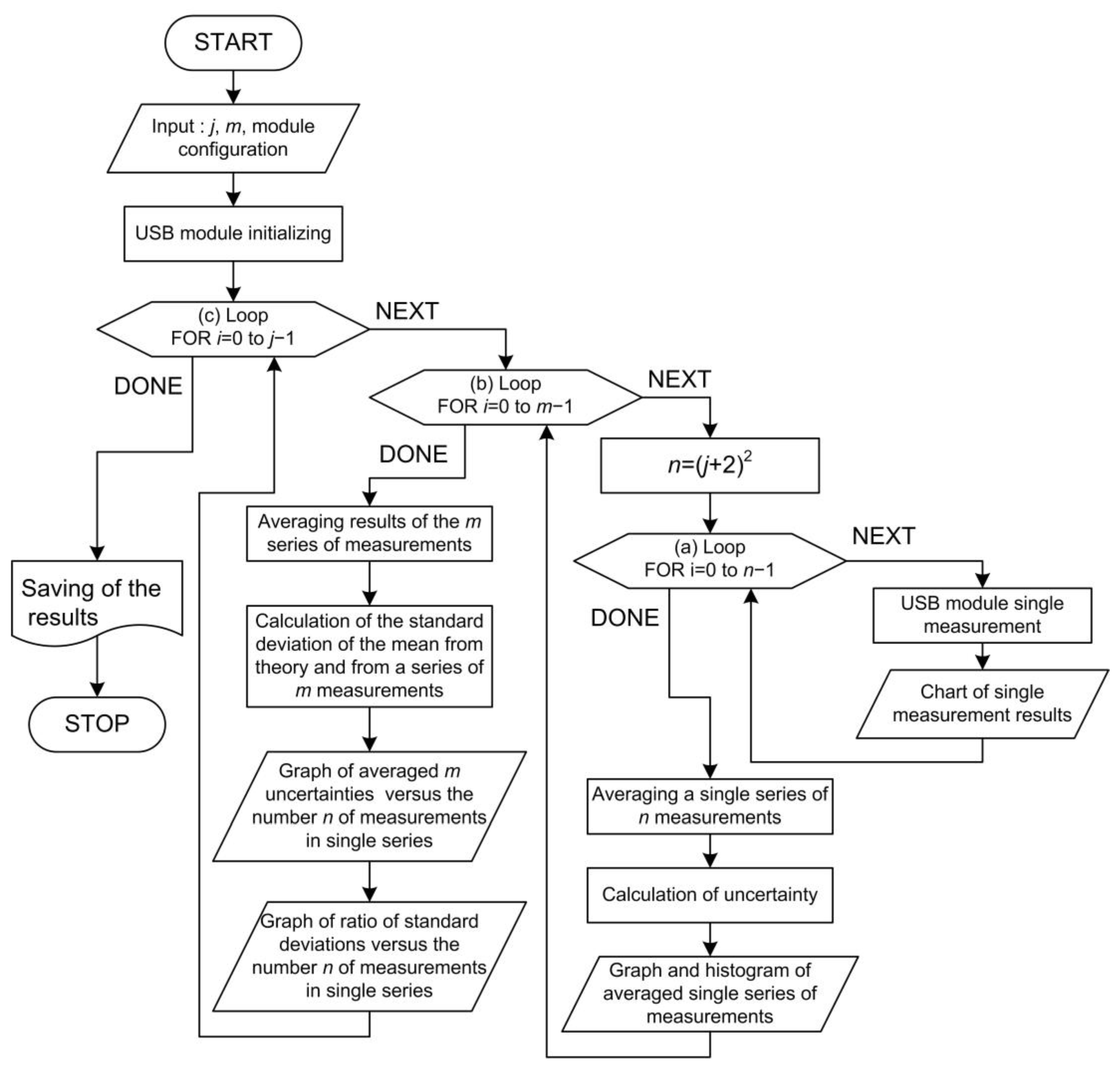
Figure 5 shows a flowchart of the algorithm that performs the measurements and calculations in the VI instrument, demonstrating the principle of the built application.
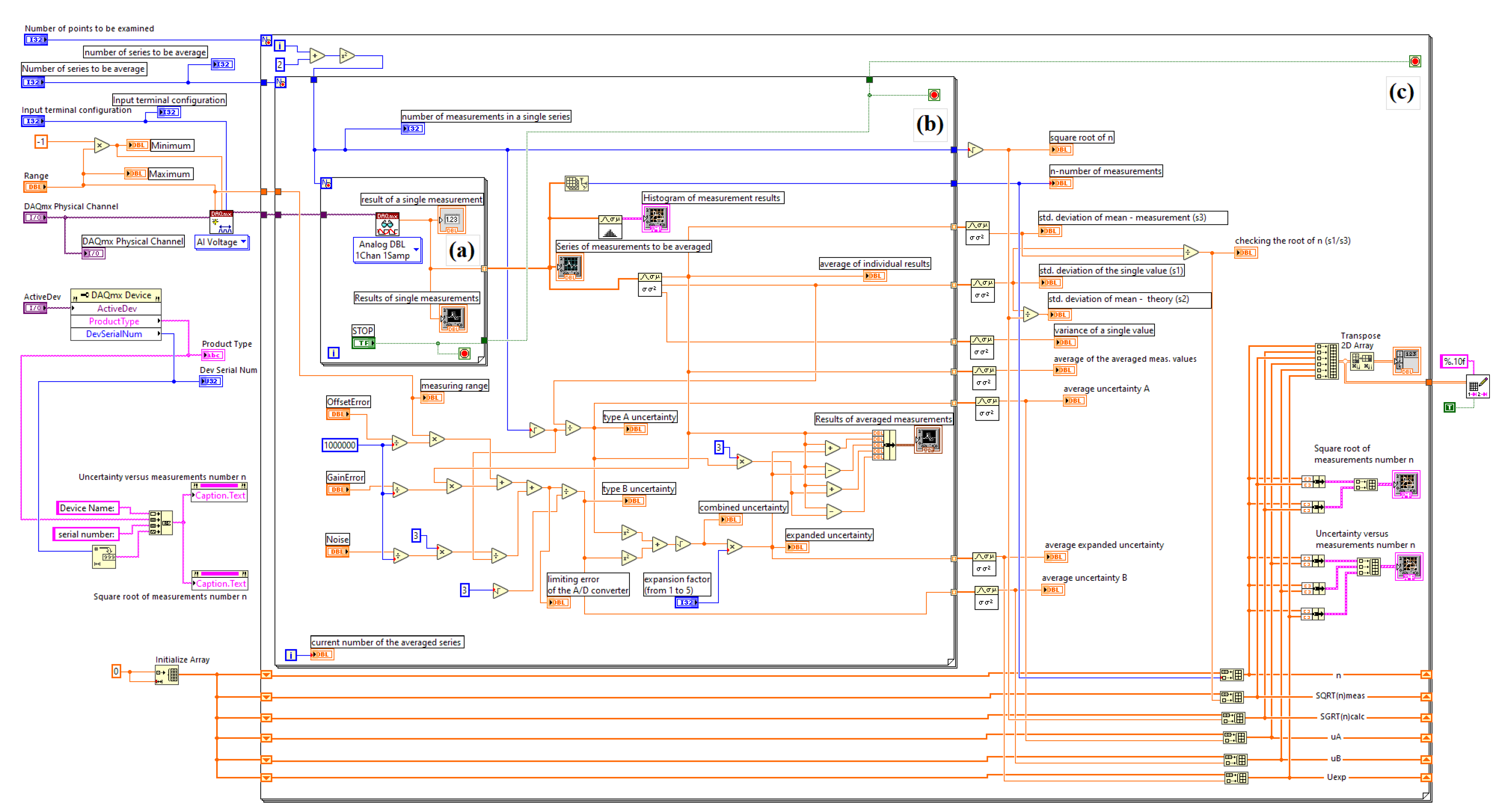
It is in the form of three FOR software loops that are mutually nested in themselves. The smaller loop (a) carries out a series of n single measurements of voltage. Figure 6 shows a LabVIEW block diagram of the developed application.
The quantity of measurements is modified automatically within a range from n = 4 to 1024, with n = (j + 2)2, where j = 0…30 is the consecutive number of the main loop flow (c). Hence, the quantity of averaged measurements assumes 31 different values but the application enables entering other values. The bigger loop (b) calls m = 100-times the lower loop (a), with the value of the arithmetic mean x ¯ from the series of n single measurements xi being computed each time [12]:
x ¯ = 1 n i = 1 n x i ,
and the experimental standard deviation s(xi) of a single result [12]:
s ( x i ) = 1 n 1 i = 1 n x i x ¯ 2 .
Type-A uncertainty is computed as an experimental standard deviation of the mean value [12]:
u A = s ( x ¯ ) = s ( x i ) n .
Type-B uncertainty is computed as a standard deviation of the rectangular distribution with a width of ±Δmpe [12]:
u B = Δ mpe 3 ,
where Δmpe is the maximum permissible error of a measuring module, computed in accordance with the documentation [20,21,22,23] based on the data contained in Table 1.
The term maximum permissible error of measurement is defined in the dictionary [14]. It should be noted that, having a reference source, a type-B experimental uncertainty could be calculated against it. However, this would limit the method to only one special case. Therefore, the maximum permissible error is calculated from the technical data of the measurement module according to the formulae and values given by the manufacturer of the measurement module. This makes the presented method more widely applicable to any type of signal source and any measuring module. The measuring modules differ in this respect. The presented system uses a standard source only as an example; any user who wishes to apply the presented method will have a different signal source and probably a different measuring module.
Finally, combined uncertainty uc [12]:
u c = u A 2 + u B 2 ,
and expanded uncertainty U are calculated [12]:
U = k u c ,
where k is the coverage factor.
Calculating the precise value of the coverage factor, for an assumed probability, is a difficult problem in the case of indirect measurements because it requires the knowledge of the function of probability density distribution of a random variable modelling the measurement result. It is a convolution of the distributions of components in the random variables that model the input quantities. Calculating convolutions is difficult and time consuming; therefore, it is a general practice to apply approximate methods.
Among the prevailing approximate methods to evaluate the coverage factor are:
(a).
Method of imposed values;
(b).
Method of effective number of degrees of freedom;
(c).
Method of geometric sum.
Ad (a) This method recommends that the coverage factor take values k(α) = 2 for the probability p  95% and k(α) = 3 for the probability p = 99.73%. It can be assumed that it is equivalent to assume the convergence of an unknown convolution of component distributions to a normal distribution. The method assumes that it is sufficient to know the confidence level approximately. Actually, the values of coverage factors should be equal for the assumed confidence levels, respectively: k(α) = 1.960 and k(α) = 2.576.
Ad (b) The method of effective number of degrees of freedom, recommended for a small number of tests (not numerous tests), is based on the Welch–Satterthwaite formula. According to the formula, if the combined standard uncertainty is a root of a sum of two or more variances estimated on the basis of results of non-numerous tests with unknown standard deviation, the unknown distribution of the required standardized variable can be approximated by means of the Student distribution for the effective number of degrees of freedom ν eff . In this method, the coverage factor k ν eff α takes values read from the tables of Student distribution for the calculated value ν eff . The value of the effective number of degrees of freedom ν eff can be determined from a general Welch–Satterthwaite equation [12]:
ν eff = u c y 4 i = 1 N y x i 4 u x i 4 ν i ,
where: u c y —standard combined uncertainty of an output quantity;
u x i —standard uncertainties of input quantities, i = 1, 2, …N;
ν i —number of degrees of freedom for a series of the measurements of input quantity.
The methods for approximating the coverage factor represented above are recommended in an inter-national document [12].
Ad (c) This is a method of algebraic sum and is frequently used in metrological practice. According to this method, we evaluate the expanded uncertainty as a geometric sum of components for the expanded uncertainties [12]:
U = i = 1 N u i 2 .
In this study, the value of the coverage factor k = 3 was adopted, according to the method of imposed values. The value of this coefficient is derived from the confidence level p = 99.73% recommended in the Guide [12].
In addition, the ratio of the averaged experimental standard deviation of a single measurement to the experimental standard deviation of the mean values in the consecutive series is computed in each flow of the main loop (c), for the consecutive values of n from n = 4 to 1024, based on the completed m = 100 of measurement series in the smaller loop (a):
s ( x i ) ¯ s ( x ¯ m ) n ,
which, theoretically, should be close to the value of n in accordance with the Equation (3) [12]. This mathematical dependence was confirmed in measurements with a low level of interferences. However, the results of measurements carried out for a high level of interferences proved a clear deviation from this theoretical dependence, which is discussed in a later part hereof.
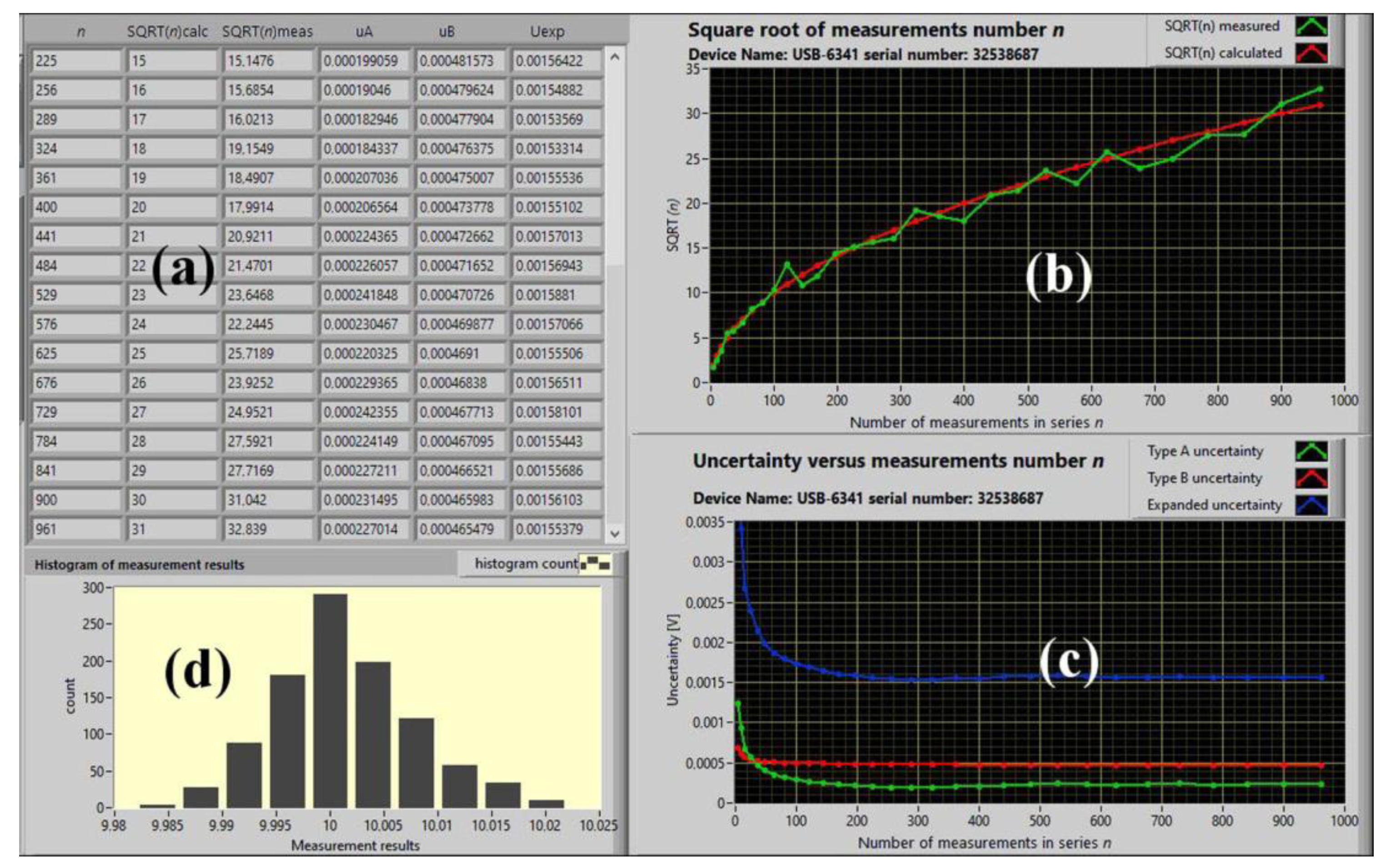
Figure 7 shows the left part of the LabVIEW application panel, which enables entering data that configure the measuring module and the manner of measurement performance (a). The middle part (b) presents the results of n measurements in the current series and the computed values of the arithmetic mean x ¯ , the maximum permissible error Δmpe, and all uncertainties. The next part (c) indicates averaged results for m = 100 completed series of n single measurements and the corresponding standard deviations of single results, standard deviations of the average value and averaged uncertainties.
Figure 8 shows the right part of the LabVIEW application panel, which presents the averaged results of computations for the consecutive series of n measurements in the form of Table (a) and in the form of Charts (b, c, d). Chart (b) presents the ratio calculated according to Equation (9), i.e., the ratio of the averaged experimental standard deviation of a single measurement to the experimental standard deviation of the mean values for consecutive series of n measurements. For the sake of comparison, Chart (b) also presents the computed values of n . Chart (c) presents type-A and -B uncertainties and expanded uncertainty U, depending on the quantity n of averaged measurements. Chart (d) presents a histogram of single results in the currently completed series of measurements. The charts are automatically complemented with the type of measuring module applied and its serial number.

3. Experimental Results

Tests of four measuring modules shown in Figure 1 were carried out on the measurement stand shown in Figure 2. Measurements were carried out with a low and a high level of interference, each time for an increased number of measurements in the series n = 4, 8, 16,…1024. For each completed series of n measurements, the software computes A-type uncertainty, B-type uncertainty and expanded uncertainty U. Each series of n measurements was repeated m = 100 times and averaged parameters were computed in order to verify the dependence (9) experimentally.

3.1. Dependence of Measurement Uncertainty on the Length of the Measurement Series

The obtained results are presented in the form of charts in Figure 9, Figure 10, Figure 11 and Figure 12. In the case of measurements with a low level of interferences (Figure 9, Figure 10, Figure 11 and Figure 12a), B-type uncertainty prevails, except for the most accurate module 6341, for which type-A uncertainty prevails in the case of a low value n < 25 (Figure 12a). In the case of less accurate modules 6008, 6001 type-B uncertainty is higher than type-A uncertainty by an order of magnitude and the averaging of a series of measurements has a relatively low effect. For n = 196, the expanded uncertainty U decreases by merely 16% for module 6008 and merely 9% for module 6001. A further extension of the series to n = 1024 no longer provides positive results. For the same conditions, the expanded uncertainty U decreases by 55% for module 6341. The lowest type-A uncertainty values were obtained for module 9215, which has BNC input slots and shielded signal wires.
In the case of measurements with a high level of interferences (Figure 9, Figure 10, Figure 11 and Figure 12b), type-A uncertainty increased uniformly for all the tested modules to a value of approx. 60 mV and was higher than type-B uncertainty by one order of magnitude. The expanded uncertainty U reached values close to 200 mV, decreasing to approx. 30 mV for the series of n = 196 measurements and to approx. 13 mV for the series of n = 1024 (for module 6341).
Furthermore, selected data are presented in Table 3 for a better comparison of the numerical values. Obviously, it must be noted that all uncertainties decrease in line with the increase in the quantity of measurements n and even with the change from n = 196 to n = 1024 expanded uncertainty U decreases by 55% more for module 6341. However, it is impossible to achieve an uncertainty that is comparable to the measurements with a low level of interferences. Note that, in the case of a high level of interference, type-A uncertainty prevails during the calculation of the expanded uncertainty U. This is due to the fact that the disturbances that occur in this measurement system are random errors, not systematic errors. At the same time, the uncertainty of type B affects the expanded uncertainty U of the measurements to a lesser extent, since it is calculated on the basis of the maximum permissible error Δmpe, which does not depend on the level of interference. The value of this error is calculated on the basis of the technical data of the measurement module provided by the manufacturer [20,21,22,23].
The method of calculating the maximum permissible error is specified by each manufacturer in the manual of the measurement module for each measurement module separately (or possibly for a series of modules). Different measuring modules, especially from different manufacturers, differ in this respect. Therefore, the documentation of a measurement module should be consulted in detail each time. Type-A uncertainty, on the other hand, depends only on the level of interference.

3.2. Effect of Length of Averaged Measurement Series on Type-A Uncertainty

When comparing the measurement results obtained for a low and a high level of interferences, it can obviously be noticed that type-A uncertainties have higher values for a high level of interferences but, simultaneously, they decrease faster, in line with the increase in the quantity of measurements n as compared to measurements with a low level of interferences. In order to examine this relationship more thoroughly, the software computes the ratio of the averaged experimental standard deviation of a single measurement to the experimental standard deviation of the arithmetic mean values in the consecutive series, according to Equation (9). Theoretically, this ratio should be close to the value of n in accordance with the dependence (3). The software presents the values of the ratio (9) obtained from the measurements in a chart, together with a chart of the calculated value of n (Figure 8b). Example charts obtained for all the tested modules, with a low and a high level of interferences, are presented in Figure 13, Figure 14, Figure 15 and Figure 16. It must be noted that the charts for the individual modules differ only slightly. Figure 13a, Figure 14a, Figure 15a and Figure 16a show charts for a low level of interferences. They indicate a very good correspondence of the ratio (9) with the value of n , which confirms the theoretical dependence (3). Figure 13b, Figure 14b, Figure 15b and Figure 16b show charts for a high level of interferences, where SQRT(n) denotes square root of n. In this case, the charts of ratio (9) lie considerably above the value of n and reach approx. twice-as-high values, hence, considerably deviating from the theoretical dependence (3). In order to examine this effect more thoroughly, the software was expanded by presentation of histograms of single results in a series of measurements.
The obtained histograms are presented in Figure 17, Figure 18, Figure 19 and Figure 20. Histograms shown in Figure 17a, Figure 18a, Figure 19a and Figure 20a for a low level of interferences are close to normal distribution, which results in a good correspondence of the results with dependence (3) in the form of charts in Figure 9a, Figure 10a, Figure 11a and Figure 12a. So-called “heavy tails” are visible in histograms shown in Figure 17b, Figure 18b, Figure 19b and Figure 20b, which means a considerable deviation from the normal distribution. The result is the absence of correspondence of the obtained measurement results with theoretical dependence (3). The standard deviation of the mean value of the measurements is lower than the theoretical value, which results in the estimation of the expanded uncertainty U that has a value that is too high [34,35,36]. This interesting issue will be the subject of further research.

4. Discussion of the Obtained Results

First, it should be noted that the aim of the presented work was not to measure the magnitude of the interference but to present the impact of the interference on the measurement process for several selected measurement modules. In this work, the expanded uncertainty was determined for several measurement modules in the presence of two levels of interference (at a low and a high interference level). It should also be noted that the design of the measurement module significantly affects the level of serial interference entering the measurement path. More expensive measurement modules, such as 6341 and 9215, which have higher resolutions and better accuracies, also have a more refined design, ensuring lower levels of serial interference. It is not only the resolution of the measurement module in terms of the number of bits that is important. Inexpensive modules, in small plastic housings, powered by a USB port, such as 6001 and 6008, are poorly resistant to interference. The 6341 module not only has a higher resolution but is important in that it has a large metal housing, where the digital and analog circuits inside are far apart. The module is powered by its own AC power supply located outside of the measurement module housing. These and other details of the module’s design result in lower interference levels. However, it was not the purpose of this manuscript to study and compare specific measurement modules. The paper presents the obtained measurement results and uncertainties. Their detailed explanation and comparison for different measurement modules would be interesting, but the conclusions obtained in this way would be limited only to the types of modules studied. Therefore, the paper presents a method and software that would allow the user to examine his own owned module in a specific application and in a specific measurement situation. The results presented by the authors are exemplary, suitable for the modules examined in the described measurement system.
Figure 9, Figure 10, Figure 11 and Figure 12 show the uncertainties obtained from the measurements for the tested modules at low levels of interference (a) and at high levels of interference (b). It can be seen that for low-interference measurements, B-type uncertainty prevails, except for the most accurate module 6341. In this case, the A-type uncertainty prevails for a small value of the average measurements n < 25. For modules 6008 and 6001, B-type uncertainty is larger than A-type uncertainty by an order of magnitude. In this case, averaging a series of measurements has a relatively small effect on type-A uncertainty. The lowest A-type uncertainty values were found for module 9215. This module has the best design, i.e., BNC-type input jacks and shielded signal cables. In the case of measurements with a high level of interference, type-A uncertainty increased uniformly for all modules tested and was one order of magnitude larger than type-B uncertainty.
Figure 13, Figure 14, Figure 15 and Figure 16 show the ratio of the experimental standard deviation of a single result in a series to the experimental deviation of the mean value of a series of n measurements related to the root of the number of measurements n for the modules tested, at low levels of interference (a) and at high levels of interference (b). The graphs for the individual modules differ only slightly. For low interference levels, they show a very good agreement between the coefficient (9) and the value of the n , confirming the theoretical relationship (3). For high interference levels, the graphs of ratio (9) lie well above the value of n , reach about twice the value, and deviate significantly from the theoretical dependence (3). Therefore, to investigate this effect in more detail, the application was extended to present histograms of individual results in a series of measurements.
Figure 17, Figure 18, Figure 19 and Figure 20 show histograms for a low level of interference (a) and a high level of interference (b). Histograms for the low level of interference are close to a normal distribution, resulting in a good correspondence of the results with the relationship (3) in the form of graphs on the left side of Figure 9, Figure 10, Figure 11 and Figure 12. For a high level of interference, there is a lack of correlation in the obtained measurement results with the theoretical relationship (3), as can be seen in the graphs on the right side of Figure 9, Figure 10, Figure 11 and Figure 12. The result is that the standard deviation of the mean value of the measurements is smaller than the theoretical value, making the estimate of the expanded uncertainty U too large, which sets a direction for further work.
When analyzing the results presented in Figure 9, Figure 10, Figure 11, Figure 12, Figure 13, Figure 14, Figure 15, Figure 16, Figure 17, Figure 18, Figure 19 and Figure 20 and in Table 3, which were obtained in this research, it can be stated that they confirmed the known theoretical relationships to a certain extent. However, the tests also indicated a significant impact of the type of interferences on the obtained results. An increase in the quantity n of averaged measurements to approx. 100–200 always results in a decrease in uncertainty for each type of module and in all conditions. A further increase in the quantity n, even up to 1000 averaged measurements, is justified only for high-accuracy modules, in particular with a high level of interferences, when type-A and -B uncertainties reach comparable values. An excessive increase in the quantity n of averaged measurements brings a particularly low effect for modules characterized by a low resolution and with a low level of interferences. The low resolution of such modules “masks” low interferences to a certain extent, which become insignificant in the measurement results and, in this case, the averaging of too many results is completely ineffective. The measurement results also proved that when estimating uncertainties, the interference probability distribution is significant, especially if it deviates from the normal distribution.

5. Conclusions

The purpose of this paper was to present a method for estimating the uncertainty of the measurement paths of A/D converters, regardless of the source and type of interference, with the paper focusing on interference from the computer power line. The range of measurement modules on the market is very wide. Users of measurement systems probably use many hundreds of types of such modules. Therefore, the authors set themselves the goal of developing a method and software that would allow the user to test the module he owns in a specific application, in a specific measurement situation. The paper presents topics concerning research on the impact of interferences on the value of uncertainties, in the case of application of measuring modules containing ADCs. It describes a developed measurement stand together with an original application created in the LabVIEW environment. The impact of the level of interferences on the value of uncertainties was determined for several selected popular measuring modules.
The test results presented in the paper should be treated as examples that are limited to the tested models of modules and to the type of interferences occurring in the measuring instrument. The essential outcome of the research is the development of a method and a system for experimental assessment of uncertainties of the measuring path with a data acquisition module, which contains an analog-to-digital converter operating in real conditions. The developed software can be applied to test any modules having appropriate drivers running in the LabVIEW environment.
It should be noted that in real measurement systems, the level of interference is not known to the user. In such a situation, the presented method allows the user of a specific measurement system to compare various possible solutions among themselves: the use of shielding, galvanic isolation, appropriate grounding, elimination of ground loops, use of different types of measurement modules. In particular, the method ensures the selection of an appropriate and optimal number of averaged measurements.
In this sense, the levels of interference occurring in the system used and the uncertainty values are only an illustration of the capabilities of the presented method and the developed application.

Author Contributions

Conceptualization, E.P., A.S. and P.O.; methodology, E.P., A.S. and P.O.; software, E.P. and A.S.; formal analysis, A.S. and P.O.; investigation, E.P., A.S. and P.O.; resources, A.S. and P.O.; writing—original draft preparation, E.P., A.S. and P.O.; writing—review and editing, E.P., A.S. and P.O.; visualization, E.P.; supervision, A.S. and P.O.; funding acquisition, A.S. All authors have read and agreed to the published version of the manuscript.

Funding

This project is financed by the Polish Ministry of Education and Science under the program “Regional Initiative of Excellence” in 2019–2023 Project number 027/RID/2018/19, amount granted PLN 11 999 900.

Data Availability Statement

All calculated, measured data and the program of LabVIEW will be provided upon request to the correspondent authors by email with appropriate justification.

Conflicts of Interest

The authors declare no conflict of interest. The funders had no role in the design of the study; in the collection, analyses, or interpretation of data; in the writing of the manuscript, or in the decision to publish the results.

References

  1. Wiczynski, G.; Kuwalek, P. Voltage Distortion Influence on Flicker Severity Measurement by AMI Energy Meters. IEEE Trans. Ind. Electron. 2021, 69, 10684–10693. [Google Scholar] [CrossRef]
  2. Wiczynski, G.; Kuwalek, P. Influence of Sampling Rate on Flicker Assessment by IEC Flickermeter Built-In AMI Energy Meters. IEEE Trans. Ind. Electron. 2021, 69, 9566–9574. [Google Scholar] [CrossRef]
  3. Kuwałek, P.; Wiczyński, G. Problem of Total Harmonic Distortion Measurement Performed by Smart Energy Meters. Meas. Sci. Rev. 2022, 22, 1–10. [Google Scholar] [CrossRef]
  4. Cipriani, G.; Miceli, R.; Spataro, C. Uncertainty evaluation in the measurements for the electric power quality analysis. In Proceedings of the 2013 International Conference on Renewable Energy Research and Applications, Madrid, Spain, 20–23 October 2013; pp. 1151–1156. [Google Scholar] [CrossRef]
  5. Lampasi, D.A.; Podesta, L. A Practical Approach to Evaluate the Measurement Uncertainty of Virtual Instruments. In Proceedings of the 21st IEEE Instrumentation and Measurement Technology Conference (IEEE Cat. No.04CH37510), Como, Italy, 18–20 May 2004; Volume 1, pp. 146–151. [Google Scholar]
  6. Bath, S.K.; Kumra, S. Simulation and Measurement of Power Waveform Distortions using LabVIEW. In Proceedings of the 2008 IEEE International Power Modulators and High-Voltage Conference, Las Vegas, NV, USA, 27–31 May 2008. [Google Scholar]
  7. Nuccio, S.; Spataro, C.; Tine, G. Virtual Instruments: Uncertainty Evaluation in the Presence of Electromagnetic Interferences. In Proceedings of the IEEE International Workshop on Advanced Methods for Uncertainty Estimation in Measurement, Sardagna, Italy, 16–18 July 2007; pp. 115–120. [Google Scholar]
  8. Arunshankar, V.K.; Kumar, N.S. Power Quality Monitoring and Control Using Virtual Instrumentation System. Power Res. J. CPRI 2014, 10, 119–124. [Google Scholar]
  9. Ghiani, E.; Locci, N.; Muscas, C. Auto-Evaluation of the Uncertainty in Virtual Instruments. IEEE Trans. Instrum. Meas. 2004, 53, 672–677. [Google Scholar] [CrossRef]
  10. Zang, C.; Wen, Y.; Wu, H. The application of the virtual instrument technology in high voltage measuring system. IEEE/PES Transm. Distrib. Conf. Exhib. 2002, 3, 2300–2304. [Google Scholar] [CrossRef]
  11. Dwivedi, V.; Singh, D. Electric Power Quality Monitoring (PQM) using Virtual Instrumentation. In Proceedings of the SPEEDAM 2010, Pisa, Italy, 14–16 June 2010; pp. 431–436. [Google Scholar] [CrossRef]
  12. JCGM 100:2008; Joint Committee for Guides in Metrology: Evaluation of Measurement Data—Guide to the Expression of Uncertainty in Measurement. BIPM Joint Committee for Guides in Metrology: Paris, France, 2008.
  13. JCGM 104:2009; Joint Committee for Guides in Metrology: Evaluation of Measurement Data—An introduction to the “Guide to the Expression of Uncertainty in Measurement” and Related Documents. BIPM Joint Committee for Guides in Metrology: Paris, France, 2009.
  14. JCGM 200:2012; Joint Committee for Guides in Metrology: International Vocabulary of Metrology—Basic and General Concepts and Associated Terms (VIM). BIPM Joint Committee for Guides in Metrology: Paris, France, 2012.
  15. EN 61000-4-8; Electromagnetic compatibility (EMC) Testing and measurement techniques. Power frequency magnetic field immunity test. International Electrotechnical Commission: Geneva, Switzerland, 2010.
  16. Otomański, P.; Pawłowski, E.; Szlachta, A. The Evaluation of Expanded Uncertainty of DC Voltages in the Presence of Electromagnetic Interferences using the LabVIEW Environment. Meas. Sci. Rev. 2021, 21, 136–141. [Google Scholar] [CrossRef]
  17. Sabat, W.; Klepacki, D.; Kamuda, K.; Kuryło, K. Analysis of LED Lamps’ Sensitivity to Surge Impulse. Electronics 2022, 11, 1140. [Google Scholar] [CrossRef]
  18. Pleština, V.; Boras, V.; Turić, H. The Measurement Uncertainty in Determining of Electrical Resistance Value by Applying Direct-Comparison Method. Energies 2022, 15, 2115. [Google Scholar] [CrossRef]
  19. Rath, M.F.; Schweighofer, B.; Wegleiter, H. Uncertainty Analysis of an Optoelectronic Strain Measurement System for Flywheel Rotors. Sensors 2021, 21, 8393. [Google Scholar] [CrossRef] [PubMed]
  20. National Instruments. USB-6001, Low-Cost DAQ USB Device, Specifications 374369A-01; National Instruments: Austin, TX, USA, 2014. [Google Scholar]
  21. National Instruments. USB-6008, 8 AI (12-Bit, 10 kS/s), 2 AO (150 Hz), 12 DIO USB Multifunction I/O Device, Specifications 375295C-01; National Instruments: Austin, TX, USA, 2017. [Google Scholar]
  22. National Instruments. USB-9215 Series, 4-Channel, ±10 VDC, 16-Bit Simultaneous Sampling Analog Input Devices, User Guide and specifications 371568E-01; National Instruments: Austin, TX, USA, 2007. [Google Scholar]
  23. National Instruments. USB-6341, 16 AI (16-Bit, 500 kS/s), 2 AO (900 kS/s), 24 DIO USB Multifunction I/O Device, Specifications 377879A-01; National Instruments: Austin, TX, USA, 2019. [Google Scholar]
  24. Zhang, J.; Xie, Y.; Huang, J.; Mo, C.; Mu, D.; Li, M. Design and simulation of reference voltage sources circuit in lasers. Microw. Opt. Technol. Lett. 2022, 1–6. [Google Scholar] [CrossRef]
  25. Texas Instruments. REF102, 10V Precision Voltage Reference, Data Sheet SBVS022B, Rev. 2009. Available online: https://www.ti.com/lit/ds/symlink/ref102.pdf?ts=1673877300040&ref_url=https%253A%252F%252Fwww.ti.com%252Fproduct%252FREF102 (accessed on 20 September 2022).
  26. Pawłowski, S.; Plewako, J. Applicability assessment for simplified formulas to compute surface impedance at screened surfaces. Przeglad Elektrotechniczny 2015, 12, 182–184. [Google Scholar] [CrossRef]
  27. National Instruments. LabVIEW User Manual, Number 320999E-01; National Instruments: Austin, TX, USA, 2003. [Google Scholar]
  28. Sokoloff, L. Applications in LabVIEW; Pearson Prentice Hall: Upper Sadle River, NJ, USA, 2004. [Google Scholar]
  29. National Instruments. LabVIEW Measurement Manual, Number 322661B-01; National Instruments: Austin, TX, USA, 2003. [Google Scholar]
  30. Otomański, P.; Szlachta, A. The Evaluation of Expanded Uncertainty of Measurement Results in Direct Measurements Using the LabVIEW Environment. Meas. Sci. Rev. 2008, 8, 147–150. [Google Scholar] [CrossRef] [Green Version]
  31. Otomański, P.; Krawiecki, Z.; Odon, A. The application of the LabVIEW environment to evaluate the accuracy of alternating voltage measurements. J. Physics: Conf. Ser. 2010, 238, 319–332. [Google Scholar] [CrossRef]
  32. Świsulski, D.; Pawłowski, E.; Dorozhovets, M. Digital Processing of Frequency–Pulse Signal in Measurement System. In Analysis and Simulation of Electrical and Computer Systems; Springer: Cham, Switzerland, 2018; pp. 319–332. [Google Scholar] [CrossRef]
  33. Pawlowski, E. Design and evaluation of a flow-to-frequency converter circuit with thermal feedback. Meas. Sci. Technol. 2017, 28, 054004–054013. [Google Scholar] [CrossRef]
  34. Dorozhovets, M. Effectiveness of Automatic Correction of Systematic Effects in Measuring Chains. Meas. Sci. Rev. 2019, 19, 132–143. [Google Scholar] [CrossRef] [Green Version]
  35. Warda, P. Simulation of an Adaptive Method of Improving the Accuracy and Extending the Range of Frequency Signal Processing in a Frequency-to-Code Converter. Appl. Sci. 2021, 11, 10341. [Google Scholar] [CrossRef]
  36. Turzeniecka, D. Errors in the evaluation of the coverage factor as a criterion of applications of approximate methods of evaluation of expanded uncertainty. Measurement 2000, 27, 223–229. [Google Scholar] [CrossRef]
Figure 1. Measurement modules tested: (a) USB-6008; (b) USB-6001; (c) USB-9215; (d) USB-6341.
Energies 16 01060 g001
Figure 2. Schematic diagram of the measurement system.
Energies 16 01060 g002
Figure 3. View of the measurement stand: 1—NI USB-6008 module; 2—NI USB-6001 module; 3—NI USB-9215 module; 4—NI-USB-6341 module; 5—REF102 reference voltage source; 6—power supply line 230 V; 7—ferromagnetic core FC; 8—signal wires; 9—USB cables; 10—computer controlling measurements; 11—application in LabVIEW environment.
Energies 16 01060 g003
Figure 4. Magnetic coupling circuit: 1—signal wire AI+; 2—signal wire AI−; 3—phase wire L; 4—neutral wire N; 5—protective wire PE; 6—ferromagnetic core, permalloy, diameter 35/55 mm, height 20 mm.
Energies 16 01060 g004
Figure 5. Flowchart of the program performing the measurements: (a) internal loop performing a series of single measurements; (b) loop repeating successive series of measurements; (c) main loop modifying the number of measurements in the series.
Energies 16 01060 g005
Figure 6. Diagram of the program performing the measurements: (a) internal loop performing a series of single measurements; (b) loop repeating successive series of measurements; (c) main loop modifying the number of measurements in the series.
Energies 16 01060 g006
Figure 7. Left panel part of the LabVIEW application: (a) data configuring measurements and uncertainty calculations; (b) results of measurements and calculations in a single series of measurements; (c) results of calculations of statistical parameters for repeatedly repeated series of measurements.
Energies 16 01060 g007
Figure 8. Right panel part of the LabVIEW application: (a) results of statistical parameter calculations for repeated multiple measurement series; (b) results of the root of the number of measurements and its verification from measurements; (c) results of measurement uncertainties type A, type B and expanded uncertainty U; (d) histogram of measurement results from a single series.
Energies 16 01060 g008
Figure 9. Uncertainties obtained from the measurements for the tested module NI USB-6008: (a) at low interference level, (b) at high interference level.
Energies 16 01060 g009
Figure 10. Uncertainties obtained from the measurements for the tested module NI USB-6001: (a) at low interference level, (b) at high interference level.
Energies 16 01060 g010
Figure 11. Uncertainties obtained from the measurements for the tested module NI USB-9215: (a) at low interference level, (b) at high interference level.
Energies 16 01060 g011
Figure 12. Uncertainties obtained from the measurements for the tested module NI USB-6341: (a) at low interference level, (b) at high interference level.
Energies 16 01060 g012
Figure 13. The ratio of the experimental standard deviation in a single result in a series to the experimental deviation of the mean value of a series of n measurements compared to the root of the number of measurements for the tested module NI USB-6008: (a) at low interference level, (b) at high interference level.
Energies 16 01060 g013
Figure 14. The ratio of the experimental standard deviation in a single result in a series to the experimental deviation of the mean value of a series of n measurements compared to the root of the number of measurements for the tested module NI USB-6001: (a) at low interference level, (b) at high interference level.
Energies 16 01060 g014
Figure 15. The ratio of the experimental standard deviation in a single result in a series to the experimental deviation of the mean value of a series of n measurements compared to the root of the number of measurements for the tested module NI USB-9215: (a) at low interference level, (b) at high interference level.
Energies 16 01060 g015
Figure 16. The ratio of the experimental standard deviation in a single result in a series to the experimental deviation of the mean value of a series of n measurements compared to the root of the number of measurements for the tested module NI USB-6341: (a) at low interference level, (b) at high interference level.
Energies 16 01060 g016
Figure 17. Histograms of individual results from a series of n = 1024 measurements made for the tested module NI USB-6008: (a) at low interference level, (b) at high interference level.
Energies 16 01060 g017
Figure 18. Histograms of individual results from a series of n = 1024 measurements made for the tested module NI USB-6001: (a) at low interference level, (b) at high interference level.
Energies 16 01060 g018
Figure 19. Histograms of individual results from a series of n = 1024 measurements made for the tested module NI USB-9215: (a) at low interference level, (b) at high interference level.
Energies 16 01060 g019
Figure 20. Histograms of individual results from a series of n = 1024 measurements made for the tested module NI USB-6341: (a) at low interference level, (b) at high interference level.
Energies 16 01060 g020
Table 1. Parameters of tested measurement modules for ±10 V differential range.
ModelResolutionGain ErrorOffset ErrorRandom ErrorLimit Error
Bitsppm of Readingppm of RangeμVrmsmV
USB 60081277350007.73
USB 6001146007006
USB 9215162001401844.535
USB 63411665132702.190
Table 2. Parameters of the REF102 BURR-BROWN reference voltage source.
Nominal VoltageMaximum ErrorTemperature DriftTime DriftNoise
10 V±2.5 mV±2.5 ppm/°C±5 ppm/1000 h5 μVpp
Table 3. Comparison of uncertainties for tested measurement modules for n = 4, 196, 1024.
ModelnLow Level of InterferenceHigh Level of Interference
uAuBUuAuBU
VVVVVV
40.002820.004460.01620.06100.00450.184
USB 60081960.000480.004460.01350.00980.00450.032
10240.000130.004460.01340.00410.00450.018
40.001460.003460.01140.05300.00350.159
USB 60011960.000220.003460.01040.00980.00350.031
10240.000100.003460.01040.00410.00350.016
40.000370.002120.00650.06600.00210.198
USB 92151960.000060.001980.00600.00970.00200.030
10240.000030.001970.00590.00420.00200.014
40.000910.000680.00350.06200.00070.186
USB 63411960.000180.000480.00160.00960.00050.029
10240.000130.000470.00150.00430.00050.013
Disclaimer/Publisher’s Note: The statements, opinions and data contained in all publications are solely those of the individual author(s) and contributor(s) and not of MDPI and/or the editor(s). MDPI and/or the editor(s) disclaim responsibility for any injury to people or property resulting from any ideas, methods, instructions or products referred to in the content.