Article

Porosity Assessment in Geological Cores Using 3D Data

1
Faculty of Geoengineering, Mining and Geology, Wroclaw University of Science and Technology, Na Grobli 15, 50-421 Wroclaw, Poland
2
Faculty of Mechanical Engineering, Wroclaw University of Science and Technology, Ignacego Łukasiewicza 5, 50-371 Wroclaw, Poland
3
3D Optical Metrology (3DOM) Unit, Bruno Kessler Foundation (FBK), Via Sommarive 18, 38121 Trento, Italy
*
Author to whom correspondence should be addressed.
Energies 2023, 16(3), 1038; https://doi.org/10.3390/en16031038
Submission received: 17 November 2022 / Revised: 26 December 2022 / Accepted: 14 January 2023 / Published: 17 January 2023
(This article belongs to the Section H3: Fossil)

Abstract

:
The porosity of rocks is an important parameter used in rock mechanics and underground mining. It affects the movement of fluids in the rock mass and the internal processes taking place (the ability to store water or gases), allowing us to characterize the type of rock and determine possible future applications. Conventional porosity testing methods (e.g., test drill cores in the laboratory) are complex and time-consuming. On the other hand, more modern technologies, such as computed tomography, are high-cost. In the presented study, a core sample with karst and porous structures inside was used. This core sample was poured with resin to reinforce the outer surfaces of the core and make it easier to cut with a rock saw. It was then cut into 3 mm thickness slices in preparation for the next step—the 3D optical scanning. Measurements were made with the ATOS CORE 500 optical scanner. Data processing was then performed in open-source software using popular and commonly used modeling methods. The 3D model of the core reconstructing the actual shape (with internal voids) and the standard model (without internal voids) were created. Based on these, the total porosity of the core was assessed. The presented solution ensures obtaining results with high accuracy at an adequate computational cost using cheap and easily available tools.

1. Introduction

The aim of the presented work is to assess the suitability of optical 3D scanning methods for digitizing geological core fragments for mechanical and morphological analyses. The presented approach focuses on the development of a rapid and relatively inexpensive method of assessing total porosity, which can be carried out in research laboratories.
Accurate geological information is very important for assessing the metal content of the ore, but also for safety reasons. Good recognition of the rock mass in terms of compressive strength allows us to select the appropriate exploiting method. In addition, precise geological information regarding, among other things, the quantity and quality of pores allows us to avoid dangerous situations such as uncontrolled leakage of gas or water into mine workings [1]. Currently, the operation of underground mines is hampered by the possibility of natural hazards in them. The constant increase in the depth of underground mines increases the possibility of gas or water hazards in them. Therefore, the exploitation of deep underground mines nowadays is associated with high risks [2,3,4,5,6].
Inflows to mines/boreholes can pose serious threats to the continuity of the exploitation of a deposit. Difficult geological and mining conditions bring increasing challenges to designers and builders, which require the use of innovative solutions to better understand the rock mass. Recognizing the material from geological boreholes allows for the proper conduct of mining operations, which is important in the context of preventing unfavorable and uncontrolled phenomena, such as flooding of pits with water, or rock and gas ejections. One of the challenges is to correctly recognize hydrogeological conditions and forecast inflows to mine workings from various parts of the rock mass. This task is simpler and yields results close to reality in systems made of porous rock (e.g., sandstone). The process becomes more difficult in carbonate rocks (e.g., limestones), in which water flow occurs in fracture or fracture-pore systems [7,8,9]. In water-bearing systems, the values of open porosity, hydraulic conductivity, and specific yield are determined and used in calculation formulas. The presence of karst voids, permeable tectonic zones, or other discontinuities that may cause sudden and unpredictable water inflows are looked for [10]. This is also a significant problem in geotechnics. In this case, the presence of water in the rocks leads to the weakening of their properties and would be related to a series of geological disasters. As numerous studies have shown, the presence of water in rock changes its mechanical properties [11,12,13,14,15]. This is an important issue in applications related to the construction of tunnels, mine workings, the construction of mine shafts, or in construction of radioactive waste disposal sites.
Misdiagnosis of geological and hydrogeological conditions leads to failures that can stop access or exploitation for months [16,17,18]. One of the methods for determining the hydrogeological parameters of rocks is to test drill cores in the laboratory. In rocks with fracture or karst flow systems, it is important to recognize the internal structure of the voids present in the examined core. From this, it is possible to draw conclusions about the nature of the connections between them, i.e. whether they are interconnected (capable of conducting water or gas) or isolated (not interconnected). Non-invasive methods such as X-ray tomography can be used [19,20,21], but despite the high spatial resolution of such devices [22,23,24], they are also high-cost [25,26]. Another method of obtaining 3D volumetric data is serial sectioning. This is a destructive technique that enables easy mechanical separation of sample sections by grinding or slicing. It then allows direct observation of the color and texture of the sample [27,28,29]. There are also methods of constructing rock models based on computer simulation, which make it possible, among other things, to simulate sedimentation processes [30]. Scanners are now widely used in various industries and in science. Commercially available scanners allow the scanning and surveying of large objects such as the geometry of underground workings. Constantly evolving technology allows us to measure smaller and smaller objects with increasing accuracy [31,32]. The authors decided to use an optical scanner to study the internal structure, which allows the examination of larger rock samples (cores). On this basis, the porosity of the analyzed rock fragment was determined and the results were compared with laboratory determinations made by traditional methods.
Optical scanners are non-contact, high-precision instruments that enable 3D reconstruction of digital data and volume assessment. They are usually equipped with sensors and one or two cameras [33]. The scanner emits light, which is then captured by the camera in the form of data reflected from the surface of the scanned object [34]. Optical scanners are widely used in almost every field: reverse engineering [35,36], healthcare [37,38], architecture [39,40], inspection [41,42], etc. The main advantages of optical scanners are high accuracy at relatively high measurement speed, as well as cost and time efficiency. Commercially available optical scanners offer accuracy on the order of hundredths of a mm (e.g., 0.037 mm for the Zeiss GOM Scan 1, 0.05 mm for the Artec Space Spider). Typically, each optical scanner manufacturer offers dedicated, specialized software for rapid measurement and post-processing of data.
In the following sections, we propose an approach based on 3D optical scanning and modeling technique to achieve digital twins of geological artifacts for virtual inspections, e.g., distribution analyses of the internal structure of voids, calculation of total porosity, etc. The method is fast and cost-effective. In the laboratory, the geological core can be quickly prepared for cutting by using resins and obtaining core fragments with homogeneous dimensions. Optical scanning and 3D modeling of such samples give knowledge of the distribution and internal structure of voids, which enables the calculation of total porosity. In future research, it will be possible to model internal structures in rocks (mainly related to karst processes), which are dangerous from the point of view of mine operations (increased water and gas inflows) and knowledge of their geometry is essential for safety.

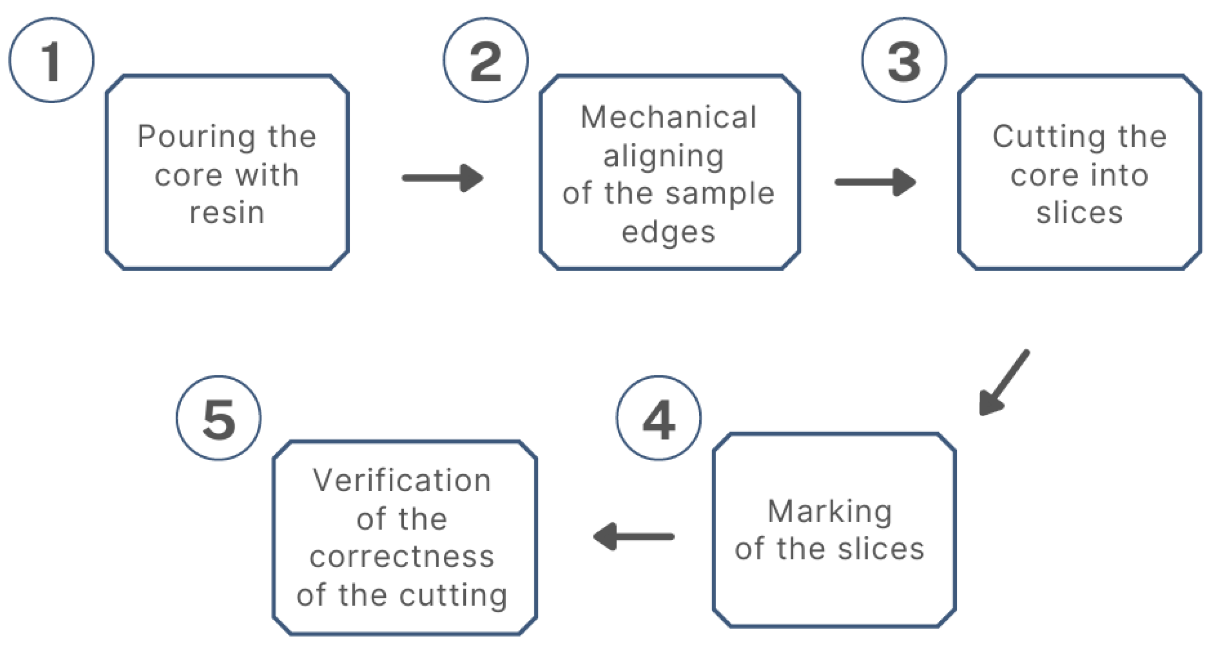
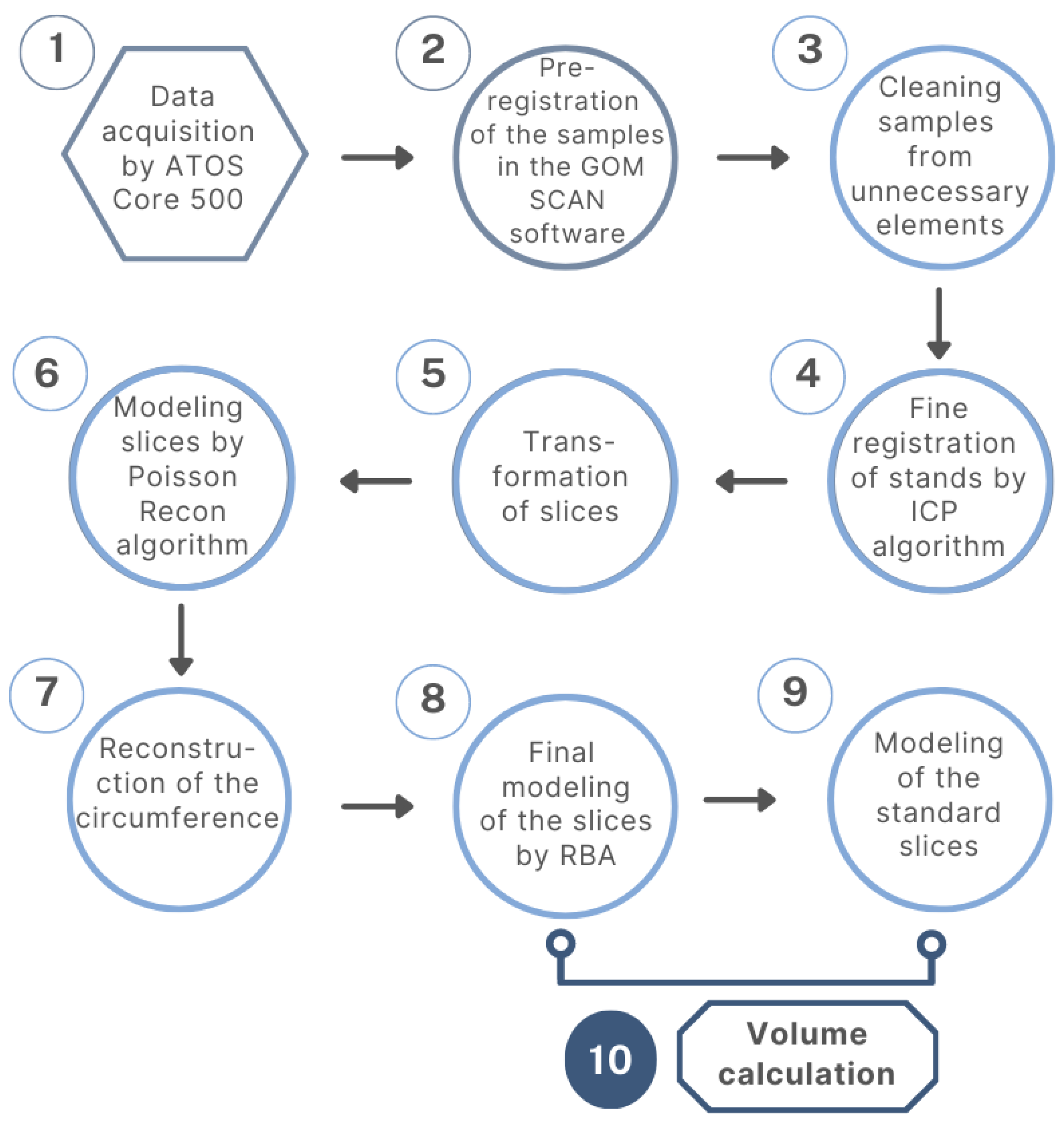
2. Materials and Methods

The research was conducted in two stages. In the first stage, the cores were prepared (cut) for testing. The second stage involved measurements using an optical scanner and 3D modeling, as described in the article.
Measurements of selected physical parameters of the core samples were carried out in the laboratory. After the boreholes were drilled, rock samples were taken from the drill cores for testing hydrogeological parameters in terms of open porosity (po) [43,44,45,46,47,48], specific yield (Sy) [44,45,47,49], and hydraulic conductivity (k) [45,47]. The samples were cylindrical in shape (diameter 50 mm; length 55 mm) (Figure 1).
First, the open porosity was determined. It determines the proportion of interconnected pores regardless of their size in the volume of the rock sample. The value of the open porosity was calculated from the formula [44,45]:
p o = ( G a G d ) G a G w · 100 %
where:
G a —the weight of the sample saturated with water (24 h) and weighed in air,
G d —the weight of the sample dried at 110 C for 24 h,
G w —the weight of the sample saturated with water (24 h) and weighed in water.
The next step in laboratory tests was the determination of specific yield ( S y ) using a high-speed centrifuge. Specific yield defines the volume of water that can drain away from a unit volume of rock [50].
The centrifuge’s speed is adjusted to the height of the sample to simulate a negative pressure of 10 m of the water column, which is assumed to be the maximum value occurring in nature and simulates natural drainage lasting 5–20 years. The S y was calculated from the formula:
S y = V w V r
where:
V w —the volume of drained water released by a suction pressure equivalent to a water column 10 m high (cm 3 ),
V r —the volume of the sample/rock (cm 3 ).
Hydraulic conductivity (k) expresses the filtration velocity at the unit hydraulic gradient if filtration follows Darcy’s linear law [51]. It depends on the rock properties (permeability) and the physical properties of water (mainly viscosity and specific gravity). Intrinsic permeability was determined in Dulinski’s [52] apparatus–gas permeameter. It works on forcing the flow of compressed gas (liquid) through the dried sample. The absolute pressure “before” and “after” the sample and the amount of gas flowing is measured. The formula is used for calculations:
k p = 2 Q p l η F ( p 1 2 p 2 2 )
where:
k p —intrinsic permeability [Darcy],
Q—the volume of flowing gas [cm 3 /s],
p—atmospheric pressure [at],
l—sample length [cm],
η —dynamic gas viscosity coefficient [cP],
F—sample cross-sectional area [cm 2 ],
p 1 —the pressure of gas before sample [at],
p 2 —the pressure of gas behind sample [at].
After the core was tested (non-destructive testing), it was further passed through manual processing in steps as shown in Figure 2. In the first step, the core was dried for 24 h at 105–110 C. Then the core was poured with resin-colored blue. The blue color was used to separate the actual rock core from the resin during the optical scanner phase of testing. After 24 h, the sunken core was given a pre-processing treatment, which consisted of aligning the bottom and top edges. The next step was to cut the core into 3 mm thick slices. The distance between consecutive slices was 3 mm and was related to the thickness of the cutting disc of the rock saw. The cut slices of rock were marked to uniquely identify their position and obverse and reverse. A measurement of the thickness of the cut core slice was made using a caliper. The procedure was repeated until the cutting of the test core was completed. After the cutting was completed, the thickness of each rock slice was summed and compared with the original core length to verify the correctness of the cutting. The sum of the slice thickness and the thickness of the cut should be equal to the length of the sample. If the difference was ± 5 % , the cutting process was considered to be correct.
The scanner used in this article, the ATOS CORE 500 (Figure 3), is based on structured blue light technology. The ATOS Core system consists of three main components: the left camera, the projector in the middle, and the right camera (Figure 3a). The technical specifications of the instrument are shown in Table 1. The cameras are based on a stereo camera configuration, which means they are calibrated to each other and the angle between them is known. The known value of the angle between the cameras enables us to determine the measuring distance from the sensor to the point of ray convergence. The measurement distance creates a three-dimensional measurement area, called the measurement volume, in which the position of 3D points can be determined. During the measurement, the sensor projects fringes onto the measured object, which are recorded by both cameras. The result is the pixel coordinates of the 3D image from the camera. In order to fully capture the object being measured, more scans are required from different positions of the object.
Reference points are used for the correct orientation of several scans in one common coordinate system. In ATOS Core, they are in the form of overlapping black and white circles of 7 mm and 3 mm in diameter. During scanning, the system determines the positions of the reference points and the distance between them as a reference point pattern. Each reference point has a coordinate and is numbered. In subsequent scans, the system recognizes the pattern and triangulates its position relative to the object’s position. To determine the sensor position, at least three reference points must always be visible for both cameras.
The process of data acquisition and processing to make 3D models and calculate the porosity of the geological core is described and presented (Figure 4) in several stages.
Step 1. The measurement with the ATOS Core 500 optical scanner was carried out for 11 samples (slices with the stand) of the core with the working number DK 402. The scanning spatial resolution was 0.19 mm. Each sample was placed in a specially constructed stand (an example of a sample is shown in Figure 5), which was permanently attached to the rotary table (Figure 3a). The stand allowed for the same position of each sample, which was important for the subsequent modeling of the entire geological core. The rotating table allowed quick scanning of the slices without the need to rotate the entire scanner system. The data of each sample was collected serially from a dozen different scanner positions, changing only the angle and height and rotating the observation object table. At this point, it should be emphasized that the resin surrounding the geological cores was not captured by the scanner, or only in painted areas.
Step 2. The capture of the scanning data and the first processing was carried out in the GOM Scan Software 2018 dedicated to the scanner used. In the program, all scans in the form of a point cloud were pre-registered, i.e., connected to one common coordinate system, using several reference points placed on the rotary table. As a result, each slice point cloud had its own local coordinate system. Due to the program’s limitations of exporting the collected data only to the triangle mesh format, the data was exported in the .stl format.
Step 3. The next step of model processing was performed in the open-source software Cloud Compare (V2.13). The 3D model of each slice was cleaned by removing unnecessary elements, such as table fragments, and residues on the resin housing, which were also scanned. The example is presented in Figure 6.
Step 4. The GOM Scan program did not allow the imposition of coordinates for reference points, so each slice model has a randomly assigned coordinate system. First, the orientation of the coordinate system was determined so that the XY plane coincides with the section plane. Then only the scanned stands (Figure 5) were used to align each model in the same reference system. Not including a slice model fragment during model registration affects better alignment and correct parameters of the final transformation. The obtained transformation parameters will give correct references to the slices. Model no. 4 was chosen as the initial model due to the best-covered scan of the stand. The “Fine Registration (ICP)” tool based on the Iterative Closest Point (ICP) algorithm was used for the aligning.
The ICP algorithm and its variants are widely used [54,55,56,57]. The first implementations of the ICP were carried out by Besl and McKay [58] and by Chen and Medioni [59]. The principle of operation is based on minimizing the root mean square distance between two point clouds or models: a reference object that is kept fixed and an object to be aligned [60]. The algorithm performs iterative rigid-body transformations as a composition of translation and rotation. The minimization error function can be written as [55]:
( R * , t * ) = a r g m i n ( i , j ) ϵ C b j R a i t 2
where:
a i —the input data points A,
b j —the input model points B,
R * —the rotation 3 × 3 matrix,
t * — the translation 3D vector.
The parameter defining the accuracy of the ICP registration performed is the RMS (root mean square) error. It is calculated based on the distance between each point in the aligned point cloud and its nearest neighbor in the cloud or reference model selected during the last iteration. The mean RMS error for the registration of the stands was 0.250 mm. The worst fit was the model of stand no. 1 with the RMS error of 0.413 mm. The error values for the registration of the rest stands are shown in Table 2.
Step 5. As mentioned in step 4, the slice models were not taken into account during the registration. A separate transformation based on the final transformation of the 4 × 4 matrix with the values obtained during the registration of the stands with the ICP algorithm was applied. This resulted in 11 overlapping models in a common coordinate system. Multiple overlapping stands were removed.
Step 6. The next step was to accurately remodel the slices, especially the pits or shadow areas that the scanner failed to capture. For each slice model, point sampling was performed on the mesh. To preserve the geometry of the scanned slices, an increased spatial resolution (0.10 mm) was used for the point clouds. At this point, the median X and Y coordinates for each slice were calculated and all values were averaged to obtain the XY center of the geological core. Therefore, all points outside the 17 mm radius that could be captured by the scanner as a resin coating were removed, resulting in point clouds in a near-cylinder shape. An example is shown in Figure 7a. Surface reconstruction was then performed using the “PoissonRecon” plug-in. It is an interface developed by Misha Kazhdan of Johns Hopkins University to generate watertight surfaces from oriented sets of points in the form of a triangle mesh, based on the Poisson formulation [61,62,63,64]. This method is commonly used for meshing [63,65], allowing not only the remeshing of existing points but also filling holes in the surface. For the analyzed sample, this function enabled modeling inaccessible pore walls or closing them. Unfortunately, the Poisson surface reconstruction technique does not perform well in modeling the circumference of the slices (Figure 7b). The algorithm bulges and rounds the circumferences, while the real model should be cylindrical.
Step 7. In order to faithfully reproduce the actual geometry of the core, the next step reconstructed the circumference of each slice based on the point clouds from step 6 with a spatial resolution of 0.10 mm. The increased spatial resolution will enable smooth modeling of the slice circumference in the next step. The perimeter lines were created as polygons object using the “2D polygon (facet)” tool for the top and bottom of the slice. This solution allows for taking into account any unevenness and pores on the edges. Then, the point cloud was created by converting polygons into points. To accurately reconstruct the circumference surface, the top and bottom perimeter lines were duplicated multiple times and shifted in the Z axis until they met at the mid-height of the slice. In this way, the point cloud representing the circumference of the slice was reconstructed. The final spatial resolution of the point cloud was 0.19 mm. Examples of the perimeter lines and the reconstructed circumference are shown in Figure 8.
Step 8. For the final slice reconstruction, the mesh model created in step 6 was converted into a point cloud with a spatial resolution of 0.19 mm. The top and bottom surfaces of the slice were cut using the perimeter lines created in the previous step. By merging the resulting point clouds of the two surfaces and the circumference, the final point cloud was prepared. The mesh model was made in the MeshLab software (V2022.02) using the “Surface reconstruction: Ball Pivoting” tool. The Ball-Pivoting Algorithm (BPA) builds a triangle mesh by rotating a circle with constant normalization on an interpolating point cloud. The process begins with a seed triangle and continues with triangulation [66,67,68]. The algorithm includes all points from the point cloud, which allows for accurate modeling of the section with the envelope. The 3D models are shown in Figure 9. The next step was to create a model that would present the true character of the geological core. Assuming a saw cut thickness of 3 mm, each successive sample was moved in the Z axis. The final model of the geological core is shown in Figure 10a.
Step 9. In order to properly calculate porosity, it is necessary to know the volume of the sample. Due to the irregularity of slice thickness, simplifying the volume using a cylindrical shape could give erroneous results. Therefore, it was decided to make standard models without voids using real models. As in step 7, a plane fit was made to the top and bottom of the slice using the “2D polygon (facet)” tools, with correction for concavity caused by the presence of pores. Finally, a point cloud was created with a minimum spatial resolution of 0.19 mm. The next step was to map the perimeter in a cylindrical shape. Here, the procedural steps were analogous to step 8. The resulting standard models without voids are shown in Figure 10b.
Step 10. The final processing process consisted of calculating the volume of the 3D models and porosity as a percentage ratio of the sum of the volume of the void to the sum of the standard model volumes. The volume of the models was calculated in MeshLab software and as a control in CloudCompare, which also has a tool for calculating geometric measures. The results from both programs were identical and are shown in Table 3.

3. Results

A core sample with karst manifestations visible on the outer walls was selected for analysis. First, non-invasive laboratory tests were performed. Then the core was coated with resin, rubbed, and examined with an optical scanner. As a result of laboratory testing of the physical parameters of the rocks, the following results were determined: open porosity (po) = 7.65%, specific yield (Sy) = 3.6, hydraulic conductivity (k) = 1.09 8 [m/s].
The data obtained from the optical scanner and processed in the software allowed for determining the volume of voids (=pores). The value obtained was 2.93% (Table 3).

4. Discussion

In this article, the authors proposed an approach to model the geometry of geological cores and assess the porosity value of the sample. The comparison of the porosity value obtained with a 3D optical scanner with that of the classic porosity measurement showed that the value was significantly lower—2 to 6 times. This comparison is not entirely correct. In the laboratory, the open porosity (po) was measured taking into account those cracks and pores that had a connection between each other and were able to conduct the medium (water, gas). The optical scanner was used to analyze the total volume of voids, which is more likely to be equated with total porosity. At this stage, the authors have not modeled the internal structure of the voids (Figure 11). Such a model would help determine which voids have connectivity with the external surfaces of the sample (open porosity) and which do not (closed porosity). Modeling of the internal structure of the voids in the core is planned in the next stages of the work.
The reasons for this difference can be found in several aspects:
(1)
The optical scanner used enables the detection of pores with the spatial resolution of the scanner, which is theoretically 0.19 mm. Observations during and after the measurement (scanning) indicate that not all holes with this minimum diameter were detected.
(2)
The slice placed in the stand during the entire scanning process is fixed on a rotating table, which provides an equal pattern of reference points and allows pre-registration. The object cannot be turned upside down to scan the innermost parts of the pores. In addition, optical scanner measurement is possible when at least three reference points are visible. Therefore, the position of the scanner position relative to the table cannot be set below its height. This makes it impossible to capture the full geometry of the holes, especially those with complex structures.
(3)
Underexposed areas are also undetectable by the scanner, which was the case for narrow and deep holes.
(4)
Incomplete capture of the holes with the scanner, especially the deeper parts, can result in erroneous surface reconstruction with the Poisson algorithm. Moreover, a void, which should be open because it occurs on several slices, may have been closed in the wrong place.
(5)
The circumferences of the slices were created using the perimeter line of the two edges of the slice: the top and bottom. They met at the mid-height of the slice. In fact, the shape of this cylinder plane should run smoothly.
(6)
Calculation of the volume of standard slices with filled voids was based on a model created by fitting planes to real surfaces. The real surfaces of the slices are not perfectly flat, and as the result, the volume was larger or absent in some places.
However, the research carried out allows us to draw some conclusions. The measurement of open porosity enables us to know the total volume of pores responsible for the conduction of water or gas in the rock environment. Due to the long time required to fill the pores with water, it is necessary to saturate the samples for a long period of time. Typically, the wet mass of a specimen increases with immersion time. The value of water absorption can be determined when a stable wet mass is achieved, which no longer increases with the immersion time [69]. In the case of sandstone, it takes about 40 h for the sample to be fully saturated with water, so the laboratory adopted a soaking time of 48 h for samples of various rocks (sedimentary, magmatic, metamorphic), allowing even the smallest spaces to be filled with water. This method of measurement is widely used to determine the water absorption capacity of rocks. It only gives quantitative information but says nothing about the internal structure of the rock voids. Observations made during other studies by the authors indicate that, depending on the shape of the voids, samples with similar open porosity show different geomechanical and conductive properties. The optical scanner method is not as accurate and has its limitations. Its advantage is that it can reproduce the size and distribution of pore spaces in the sample despite the fertility limitations. The development of optical analysis methods combined with modeling of the internal structure of voids will enable the separation of open porosity from total porosity for a given sample in subsequent steps. These issues are important for assessing gas hazards in the rock mass in a mine. They will also allow the modeling of the amount of gas that can be released from the rock mass after blasting.
Future research should focus on modeling the voids created after cutting. Accurate modeling of voids inside cores and more accurate determination of porosity are also areas of great research potential.

5. Conclusions

The laboratory methods currently used to determine porosity are used to measure open porosity. These measurements give information about the number of permeable pores in relation to the volume of the test sample. The results of these analyses are widely used in various calculation methods for estimating inflow to pits, shafts, or mine workings. Assessment of karst and fracture structures in rock samples has rarely been undertaken to date. This was due to the lack of appropriate testing tools. The development of optical scanning methods and computer scan processing opens up new possibilities for the analysis karst fracture structures in rock samples. In addition, it is a fast and effective method based on low-cost equipment and software. Other modern techniques, such as X-ray computed tomography imaging, despite their high accuracy and time efficiency, are significantly costly, making them difficult to access and limited in availability. The method proposed by the authors is based on relatively cheap and available measurement equipment and open-source software that can be used by non-experts.
The research presented here has a preliminary character, for validating the method for assessing the shape and size of voids that occur inside a rock sample.The team’s further work will focus on developing algorithms to reconstruct the rock surface and build an internal model of voids in the sample. This data can then be used to model the flow of water or gases in the rock environment to better predict dangerous phenomena in mines or tunnels. This will open up new possibilities for assessing rock mass formation and selecting rational dewatering methods.

Author Contributions

Conceptualization, P.K. and K.C.; methodology, P.K. and K.C.; software, P.K., K.L. and A.B.; formal analysis, P.K. and K.C.; investigation, P.K. and K.C.; resources, K.C.; writing—original draft preparation, P.K. and K.C.; writing—review and editing, P.K., K.C. and A.B.; visualization, P.K. and K.L.; supervision, R.Z. and F.R. All authors have read and agreed to the published version of the manuscript.

Funding

This research received no external funding.

Data Availability Statement

The data presented in this study are available on request from the corresponding author.

Conflicts of Interest

The authors declare no conflict of interest.

Abbreviations

The following abbreviations are used in this manuscript:
BPABall-Pivoting Algorithm
ICPIterative Closest Point
RMSRoot Mean Square

References

  1. Lu, J.; Meng, X.; Wang, Y.; Yang, Z. Prediction of coal seam details and mining safety using multicomponent seismic data: A case history from China. Geophysics 2016, 81, B149–B165. [Google Scholar] [CrossRef]
  2. Kozieł, K.; Skoczylas, N.; Soroko, K.; Gola, S. Gas and Dolomite Outbursts in Ore Mines—Analysis of the Phenomenon and the Energy Balance. Energies 2020, 13, 2999. [Google Scholar] [CrossRef]
  3. Dong, L.; Tong, X.; Li, X.; Zhou, J.; Wang, S.; Liu, B. Some developments and new insights of environmental problems and deep mining strategy for cleaner production in mines. J. Clean. Prod. 2019, 210, 1562–1578. [Google Scholar] [CrossRef]
  4. Ziętek, B.; Banasiewicz, A.; Zimroz, R.; Szrek, J.; Gola, S. A Portable Environmental Data-Monitoring System for Air Hazard Evaluation in Deep Underground Mines. Energies 2020, 13, 6331. [Google Scholar] [CrossRef]
  5. Hebda-Sobkowicz, J.; Gola, S.; Zimroz, R.; Wyłomańska, A. Pattern ofH2Sconcentration in a deep copper mine and its correlation with ventilation schedule. Measurement 2019, 140, 373–381. [Google Scholar] [CrossRef]
  6. Liu, Z.; Zhao, R.; Dong, S.; Wang, W.; Sun, H.; Mao, D. Scanning for water hazard threats with sequential water releasing tests in underground coal mines. J. Hydrol. 2020, 590, 125350. [Google Scholar] [CrossRef]
  7. Bocheńska, T.; Fiszer, J.; Kalisz, M. Prediction of groundwater inflow into copper mines of the Lubin Glogow Copper District. Environ. Geol. 2000, 39, 587–594. [Google Scholar] [CrossRef]
  8. Motyka, J.; Czop, M. Influence of Karst Phenomena on Water Inflow to Zn-Pb Mines in the Olkusz District (S Poland). Environ. Earth Sci. 2010, 449–454. [Google Scholar] [CrossRef]
  9. Liu, J.; Zhao, Y.; Tan, T.; Zhang, L.; Zhu, S.; Xu, F. Evolution and modeling of mine water inflow and hazard characteristics in southern coalfields of China: A case of Meitanba mine. Int. J. Min. Sci. Technol. 2022, 32, 513–524. [Google Scholar] [CrossRef]
  10. Bonacci, O.; Ljubenkov, I.; Roje-Bonacci, T. Karst flash floods: An example from the Dinaric karst (Croatia). Nat. Hazards Earth Syst. Sci. 2006, 6, 195–203. [Google Scholar] [CrossRef]
  11. Krokosky, E.M.; Husak, A. Strength characteristics of basalt rock in ultra-high vacuum. J. Geophys. Res. 1968, 73, 2237–2247. [Google Scholar] [CrossRef]
  12. Szlavin, J. Relationships between some physical properties of rock determined by laboratory tests. Int. J. Rock Mech. Min. Sci. Geomech. Abstr. 1974, 11, 57–66. [Google Scholar] [CrossRef]
  13. Van Eeckhout, E.M.; Peng, S.S. The effect of humidity on the compliances of coal mine shales. Int. J. Rock Mech. Min. Sci. Geomech. Abstr. 1975, 12, 335–340. [Google Scholar] [CrossRef]
  14. Li, G.C.; Qi, C.C.; Sun, Y.T.; Tang, X.L.; Hou, B.Q. Experimental Study on the Softening Characteristics of Sandstone and Mudstone in Relation to Moisture Content. Shock Vib. 2017, 2017, 4010376. [Google Scholar] [CrossRef] [Green Version]
  15. Shen, Y.J.; Wang, Y.Z.; Zhao, X.D.; Yang, G.S.; Jia, H.L.; Rong, T.L. The influence of temperature and moisture content on sandstone thermal conductivity from a case using the artificial ground freezing(AGF) method. Cold Reg. Sci. Technol. 2018, 155, 149–160. [Google Scholar] [CrossRef]
  16. Kalisz, M.; Niedbał, M. Wpływ odwadniania utworów triasowych w trakcie głȩbienia szybu R–XI na warunki hydrodynamiczne i powierzchniowe w północnej czȩści OG “Rudna”. In Materiały Sympozjum Naukowo–Technicznego “Problemy Hydrogeologiczne Górnictwa Rud Miedzi”; KGHM Polska Miedź S.A.: Lubin, Poland, 2004; pp. 148–160. [Google Scholar]
  17. Butra, J. Rozwój górnictwa rud miedzi [Development in copper ore mining]. Rudy i Metale Nieżelazne 2005, 50, 481–484. [Google Scholar]
  18. Chudy, K.; Worsa-Kozak, M.; Pikuła, M. Rozwój metod rozpoznania warunków hydrogeologicznych na potrzeby wykonywania pionowych wyrobisk udostȩpniaja̧cych złoże–przykład LGOM. Przegla̧d Geologiczny 2017, 65, 1035–1043. [Google Scholar]
  19. Taud, H.; Martinez-Angeles, R.; Parrot, J.; Hernandez-Escobedo, L. Porosity estimation method by X-ray computed tomography. J. Pet. Sci. Eng. 2005, 47, 209–217. [Google Scholar] [CrossRef]
  20. Galkin, S.; Efimov, A.; Krivoshchekov, S.; Savitskiy, Y.; Cherepanov, S. X-ray tomography in petrophysical studies of core samples from oil and gas fields. Russ. Geol. Geophys. 2015, 56, 782–792. [Google Scholar] [CrossRef]
  21. Romano, C.; Minto, J.M.; Shipton, Z.K.; Lunn, R.J. Automated high accuracy, rapid beam hardening correction in X-Ray Computed Tomography of multi-mineral, heterogeneous core samples. Comput. Geosci. 2019, 131, 144–157. [Google Scholar] [CrossRef]
  22. Geiger, J.; Hunyadfalvi, Z.; Bogner, P. Analysis of small-scale heterogeneity in clastic rocks by using computerized X-ray tomography (CT). Eng. Geol. 2009, 103, 112–118. [Google Scholar] [CrossRef]
  23. Sergeevich, O.M.; Valeriyevich, R.P.; Aleksandrovich, S.I.; Tarasovich, L.V. The application of X-ray Micro Computed Tomography (Micro-CT) of core sample for estimation of physicochemical treatment efficiency. In Proceedings of the SPE Russian Petroleum Technology Conference, Moscow, Russia, 26–28 October 2015. [Google Scholar]
  24. Zhang, P.; Lee, Y.I.; Zhang, J. A review of high-resolution X-ray computed tomography applied to petroleum geology and a case study. Micron 2019, 124, 102702. [Google Scholar] [CrossRef] [PubMed]
  25. Bai, Y.; Berezovsky, V.; Popov, V. Digital core 3d reconstruction based on micro-ct images via a deep learning method. In Proceedings of the 2020 International Conference on High Performance Big Data and Intelligent Systems (HPBD&IS), Shenzhen, China, 23 May 2020; pp. 1–6. [Google Scholar]
  26. Liu, D.; Zhao, Z.; Cai, Y.; Sun, F.; Zhou, Y. Review on Applications of X-ray Computed Tomography for Coal Characterization: Recent Progress and Perspectives. Energy Fuels 2022, 36, 6659–6674. [Google Scholar] [CrossRef]
  27. Wiltsche, M.; Donoser, M.; Kritzinger, J.; Bauer, W. Automated serial sectioning applied to 3D paper structure analysis. J. Microsc. 2011, 242, 197–205. [Google Scholar] [CrossRef]
  28. Echlin, M.P.; Burnett, T.L.; Polonsky, A.T.; Pollock, T.M.; Withers, P.J. Serial sectioning in the SEM for three dimensional materials science. Curr. Opin. Solid State Mater. Sci. 2020, 24, 100817. [Google Scholar] [CrossRef]
  29. Mehra, A.; Howes, B.; Manzuk, R.; Spatzier, A.; Samuels, B.M.; Maloof, A.C. A Novel Technique for Producing Three-Dimensional Data Using Serial Sectioning and Semi-Automatic Image Classification. Microsc. Microanal. 2022, 28, 2020–2035. [Google Scholar] [CrossRef] [PubMed]
  30. Luo, M.; Glover, P.W.; Zhao, P.; Li, D. 3D digital rock modeling of the fractal properties of pore structures. Mar. Pet. Geol. 2020, 122, 104706. [Google Scholar] [CrossRef]
  31. Szrek, J.; Zimroz, R.; Wodecki, J.; Michalak, A.; Góralczyk, M.; Worsa-Kozak, M. Application of the Infrared Thermography and Unmanned Ground Vehicle for Rescue Action Support in Underground Mine—The AMICOS Project. Remote Sens. 2020, 13, 69. [Google Scholar] [CrossRef]
  32. Wróblewski, A.; Wodecki, J.; Trybała, P.; Zimroz, R. A Method for Large Underground Structures Geometry Evaluation Based on Multivariate Parameterization and Multidimensional Analysis of Point Cloud Data. Energies 2022, 15, 6302. [Google Scholar] [CrossRef]
  33. Haleem, A.; Gupta, P.; Bahl, S.; Javaid, M.; Kumar, L. 3D scanning of a carburetor body using COMET 3D scanner supported by COLIN 3D software: Issues and solutions. Mater. Today Proc. 2021, 39, 331–337. [Google Scholar] [CrossRef]
  34. Javaid, M.; Haleem, A.; Pratap Singh, R.; Suman, R. Industrial perspectives of 3D scanning: Features, roles and it’s analytical applications. Sensors Int. 2021, 2, 100114. [Google Scholar] [CrossRef]
  35. Sedlak, J.; Polzer, A.; Chladil, J.; Slany, M.; Jaros, A. Reverse engineering method used for inspection of stirrer´s gearbox cabinet prototype. MM Sci. J. 2017, 2017, 1877–1882. [Google Scholar] [CrossRef]
  36. Bernal, C.; De Agustina, B.; Marín, M.M.; Camacho, A.M. Performance evaluation of optical scanner based on blue LED structured light. Procedia Eng. 2013, 63, 591–598. [Google Scholar] [CrossRef] [Green Version]
  37. Petrides, G.; Clark, J.R.; Low, H.; Lovell, N.; Eviston, T.J. Three-dimensional scanners for soft-tissue facial assessment in clinical practice. J. Plast. Reconstr. Aesthetic Surg. 2021, 74, 605–614. [Google Scholar] [CrossRef] [PubMed]
  38. Ye, H.; Lv, L.; Liu, Y.; Liu, Y.; Zhou, Y. Evaluation of the Accuracy, Reliability, and Reproducibility of Two Different 3D Face-Scanning Systems. Int. J. Prosthodont. 2016, 29, 213–218. [Google Scholar] [CrossRef] [PubMed]
  39. Iuliano, L.; Minetola, P. Rapid manufacturing of sculptures replicas: A comparison between 3D optical scanners. In Proceedings of the CIPA 2005 XX International Symposium, Torino, Italy, 26 September–1 October 2005; Volume 26. [Google Scholar]
  40. Rocchini, C.; Cignoni, P.; Montani, C.; Pingi, P.; Scopigno, R. A low cost 3D scanner based on structured light. Comput. Graph. Forum 2001, 20, 299–308. [Google Scholar] [CrossRef]
  41. Lazarević, D.; Nedić, B.; Jović, S.; Šarkoćević, Ž.; Blagojević, M. Optical inspection of cutting parts by 3D scanning. Phys. A Stat. Mech. Appl. 2019, 531, 121583. [Google Scholar] [CrossRef]
  42. Brajlih, T.; Tasic, T.; Igor, D.; Valentan, B.; Hadžistević, M.; Pogačar, V.; Balic, J.; Acko, B. Possibilities of Using Three-Dimensional Optical Scanning in Complex Geometrical Inspection. Strojniški Vestnik 2011, 57, 826–833. [Google Scholar] [CrossRef] [Green Version]
  43. Duguid, J.O.; Lee, P.C.Y. Flow in Fractured Porous Media. Water Resour. Res. 1977, 13, 558–566. [Google Scholar] [CrossRef]
  44. Motyka, J.; Pulido-Bosch, A. Karstic phenomena in calcareous-dolomitic rocks and their influence over the inrushes of water in lead-zinc mines in Olkusz region (South of Poland). Int. J. Mine Water 1985, 4, 1–11. [Google Scholar] [CrossRef]
  45. Motyka, J.; Pulido-Bosch, A.; Borczak, S.; Gisbert, J. Matrix hydrogeological properties of Devonian carbonate rocks of Olkusz (Southern Poland). J. Hydrol. 1998, 211, 140–150. [Google Scholar] [CrossRef]
  46. Borczak, S.; Motyka, J.; Pulido-Bosch, A. The hydrogeological properties of the matrix of the chalk in the Lublin coal basin (southeast Poland). Hydrol. Sci. J. 1990, 35, 523–534. [Google Scholar] [CrossRef]
  47. Motyka, J. A conceptual model of hydraulic networks in carbonate rocks, illustrated by examples from Poland. Hydrogeol. J. 1998, 6, 469–482. [Google Scholar] [CrossRef]
  48. Zuber, A.; Motyka, J. Matrix porosity as the most important parameter of fissured rocks for solute transport at large scales. J. Hydrol. 1994, 158, 19–46. [Google Scholar] [CrossRef]
  49. Motyka, J.; Postawa, A. Influence of contaminated Vistula River water on the groundwater entering the Zakrzowek limestone quarry, Cracow region, Poland. Environ. Geol. 2000, 39, 398–404. [Google Scholar] [CrossRef]
  50. Todd, D.K.; Mays, L.W. Groundwater Hydrology, 3rd ed.; John Wiley & Sons Inc.: Hoboken, NJ, USA, 2004; pp. 1–656. [Google Scholar]
  51. Dowgiałło, J.; Kleczkowski, A.; Macioszczyk, T.; Różkowski, A. Słownik Hydrogeologiczny [Hydrogeological Dictionary]; Państwowego Instytutu Geologicznego: Warszawa, Poland, 2002; p. 461. [Google Scholar]
  52. Duliński, W. Aparat do Badania Przepuszczalności z Uszczelnieniem Pneumatycznym; Wiadomości Naftowe: Kraków, Poland, 1965; Volume 7, pp. 117–118. [Google Scholar]
  53. ATOS Core Optical 3D Scanner for Quality Control. Brochure. 2020. Available online: https://scanare3d.com/wp-content/uploads/2020/07/GOM_Brochure_ATOS_Core_EN.pdf, (accessed on 16 January 2023).
  54. Zhang, Z. Iterative point matching for registration of free-form curves and surfaces. Int. J. Comput. Vis. 1994, 13, 119–152. [Google Scholar] [CrossRef]
  55. Zinßer, T.; Schmidt, J.; Niemann, H. Point set registration with integrated scale estimation. In Proceedings of the International Conference on Pattern Recognition and Image Processing, Bath, UK, 22–25 August 2005; pp. 116–119. [Google Scholar]
  56. Pomerleau, F.; Colas, F.; Siegwart, R. A review of point cloud registration algorithms for mobile robotics. Found. Trends® Robot. 2015, 4, 1–104. [Google Scholar] [CrossRef] [Green Version]
  57. Tombari, F.; Remondino, F. Feature-based automatic 3D registration for cultural heritage applications. In Proceedings of the 2013 Digital Heritage International Congress (DigitalHeritage), Marseille, France, 28 October–1 November 2013; Volume 1, pp. 55–62. [Google Scholar] [CrossRef]
  58. Besl, P.; McKay, N.D. A method for registration of 3-D shapes. IEEE Trans. Pattern Anal. Mach. Intell. 1992, 14, 239–256. [Google Scholar] [CrossRef] [Green Version]
  59. Chen, Y.; Medioni, G. Object modelling by registration of multiple range images. Image Vis. Comput. 1992, 10, 145–155. [Google Scholar] [CrossRef]
  60. Rusinkiewicz, S.; Levoy, M. Efficient variants of the ICP algorithm. In Proceedings of the Third International Conference on 3-D Digital Imaging and Modeling, Quebec City, QC, Canada, 28 May–1 June 2001; pp. 145–152. [Google Scholar]
  61. Kazhdan, M.; Bolitho, M.; Hoppe, H. Poisson Surface Reconstruction. In Proceedings of the Symposium on Geometry Processing; Sheffer, A., Polthier, K., Eds.; The Eurographics Association: Eindhoven, The Netherlands, 2006. [Google Scholar] [CrossRef]
  62. Kazhdan, M.; Hoppe, H. Screened poisson surface reconstruction. ACM Trans. Graph. 2013, 32, 1–13. [Google Scholar] [CrossRef]
  63. Alexiou, E.; Bernardo, M.V.; Da Silva Cruz, L.A.; Dmitrovic, L.G.; Duarte, C.; Dumic, E.; Ebrahimi, T.; Matkovic, D.; Pereira, M.; Pinheiro, A.; et al. Point Cloud Subjective Evaluation Methodology based on 2D Rendering. In Proceedings of the 2018 10th International Conference on Quality of Multimedia Experience, QoMEX 2018, Sardinia, Italy, 29–31 May 2018. [Google Scholar] [CrossRef] [Green Version]
  64. Kazhdan, M.; Chuang, M.; Rusinkiewicz, S.; Hoppe, H. Poisson Surface Reconstruction with Envelope Constraints. Eurographics Symp. Geom. Process. 2020, 39, 173–182. [Google Scholar] [CrossRef]
  65. Nocerino, E.; Stathopoulou, E.K.; Rigon, S.; Remondino, F. Surface Reconstruction Assessment in Photogrammetric Applications. Sensors 2020, 20, 5863. [Google Scholar] [CrossRef] [PubMed]
  66. Bernardini, F.; Mittleman, J.; Rushmeier, H.; Silva, C.; Taubin, G. The ball-pivoting algorithm for surface reconstruction. IEEE Trans. Vis. Comput. Graph. 1999, 5, 349–359. [Google Scholar] [CrossRef]
  67. Cignoni, P.; Callieri, M.; Corsini, M.; Dellepiane, M.; Ganovelli, F.; Ranzuglia, G. MeshLab: An Open-Source Mesh Processing Tool. In Proceedings of the Eurographics Italian Chapter Conference, Salerno, Italy, 2–4 July 2008; Volume 2008, pp. 129–136. [Google Scholar]
  68. Mariosa, G.; Fioraio, N.; Franchi, A.; Stefano, L.D. Surface Reconstruction from Range Images. In Proceedings of the Smart Tools and Apps for Graphics–Eurographics Italian Chapter Conference; Pintore, G., Stanco, F., Eds.; The Eurographics Association: Eindhoven, The Netherlands, 2016. [Google Scholar] [CrossRef]
  69. Wong, L.N.Y.; Maruvanchery, V.; Liu, G. Water effects on rock strength and stiffness degradation. Acta Geotech. 2016, 11, 713–737. [Google Scholar] [CrossRef]
Figure 1. Rock cutting saw (left), core before cutting (center) and some examples of sliced core (right).
Energies 16 01038 g001
Figure 2. Scheme of manual preparing the sample.
Energies 16 01038 g002
Figure 3. The measurement system with the rotating table (a) and the optical scanner (b).
Energies 16 01038 g003
Figure 4. Scheme of data processing for modeling and calculation of volume and porosity of the geological core.
Energies 16 01038 g004
Figure 5. Slice no. 7 placed in the stand on the rotating table at the front (a) and rear (b) view.
Energies 16 01038 g005
Figure 6. Model of slice no. 7 before (a) and after (b) removing unnecessary elements.
Energies 16 01038 g006
Figure 7. The point cloud (a) and the 3D mesh model created by Poisson surface reconstruction (b) of slice no. 7.
Energies 16 01038 g007
Figure 8. The perimeter lines fitted in the top and bottom of slice (a) and the reconstructed circumference (b) of slice no. 7.
Energies 16 01038 g008
Figure 9. The 3D models of the individual slices of DK 402 sample.
Energies 16 01038 g009aEnergies 16 01038 g009b
Figure 10. The real 3D model of the sample with voids (a) and the standard 3D model without voids (b).
Energies 16 01038 g010
Figure 11. Visualization of the problem of the lack of modeled internal structure of voids.
Energies 16 01038 g011
Table 1. Technical data of ATOS Core 500 (based on [53]).
Measuring area [mm]500 × 380
Working distance [mm]440
Sensor dimensions [mm]361 × 205 × 64
Spatial resolution [mm]0.19 (0.31) *
Weight [kg]2.9
Temperature range [°C]+5 to +40, non-condensing
Power supply [V]90–230
* GOM Scan with Sensor Driver 2M.
Table 2. The RMS value of registration for the stands.
No. of Slice and StandRMS Value [mm]
no. 10.413
no. 20.294
no. 30.263
no. 4-
no. 50.205
no. 60.203
no. 70.206
no. 80.211
no. 90.223
no. 100.210
no. 110.269
MEAN:0.250
Table 3. The values of volume of each slice and internal voids for standard (without voids) and real models (with voids).
Standard (without Voids) [mm 3 ]Real (with Voids) [mm 3 ]Voids [mm 3 ]
no. 12722.922722.360.57
no. 22021.991985.4136.58
no. 32291.522214.0977.43
no. 42287.052228.7958.26
no. 52402.192296.07106.12
no. 62131.822117.9513.87
no. 72291.452267.8923.57
no. 82753.072542.97210.10
no. 92343.452259.6583.80
no. 102753.882674.0879.80
no. 112044.861971.8273.04
26,044.2125,281.08763.13
100%97.07%2.93%
Disclaimer/Publisher’s Note: The statements, opinions and data contained in all publications are solely those of the individual author(s) and contributor(s) and not of MDPI and/or the editor(s). MDPI and/or the editor(s) disclaim responsibility for any injury to people or property resulting from any ideas, methods, instructions or products referred to in the content.

