
Collaborative Optimal Configuration of a Mobile Energy Storage System and a Stationary Energy Storage System to Cope with Regional Grid Blackouts in Extreme Scenarios


Abstract
:1. Introduction
- A model for the joint configuration of MESS and SESS has been established, which has fully utilized the respective advantages of the two types of energy storage systems, resulting in improved economic benefits for the optimization results.
- Considering the load recovery, the reliability constraint is established in this paper, which can ensure that the energy storage configuration results can meet the load recovery requirements.
- Given the randomness of extreme scenarios, the randomness has been addressed through the method of scenario analysis, allowing the configuration results to adapt to multiple scenarios for operational efficiency.
2. Mobile Energy Storage System
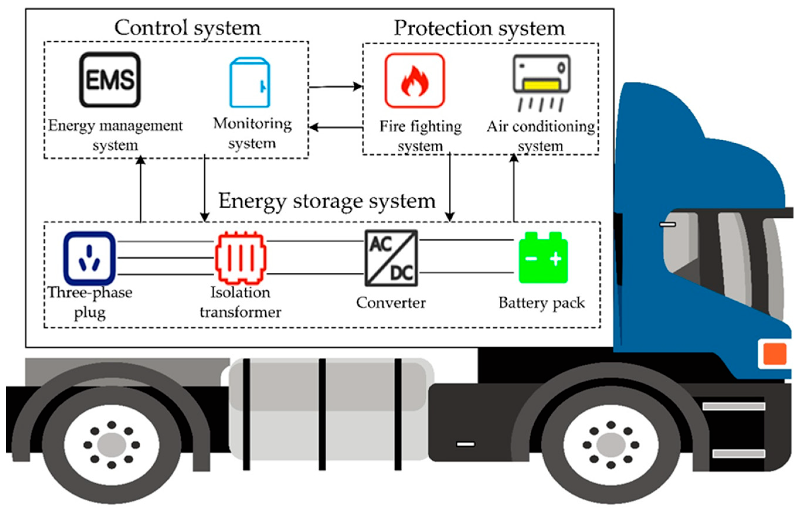
2.1. Structure of MESS
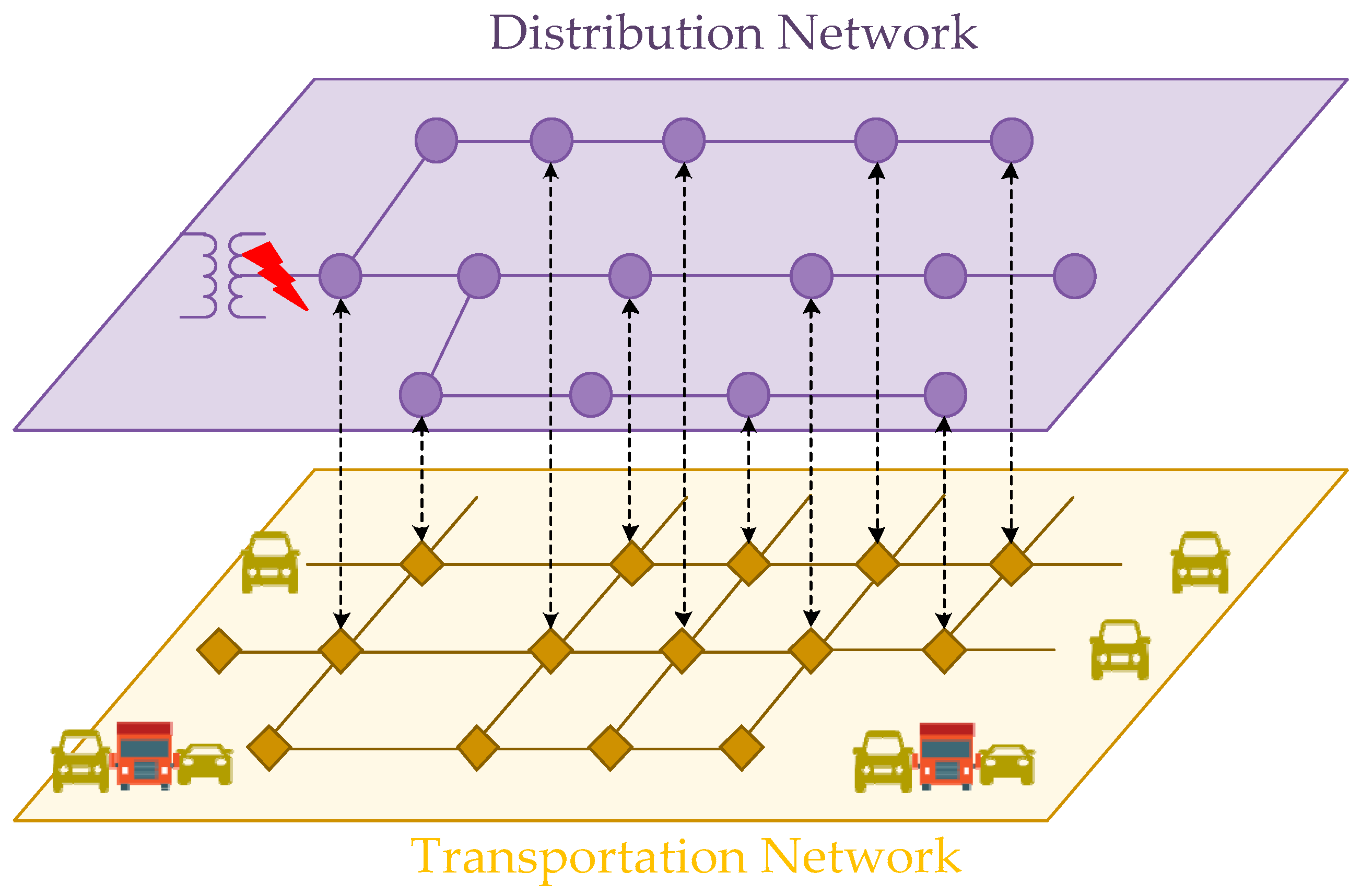
2.2. MESS Space–Time Scheduling Model
2.3. MESS Operational Constraint Model
3. Configuration Model
3.1. Objective Function
3.1.1. Investment Cost
3.1.2. Operation and Maintenance Cost
3.1.3. Load Shedding Penalty Cost
3.2. SESS Operation Constraint Model
3.3. Reliability Constraint
3.4. Other Constraints
3.4.1. Distributed Generation
3.4.2. Power Balance
3.4.3. Power Flow Constraints
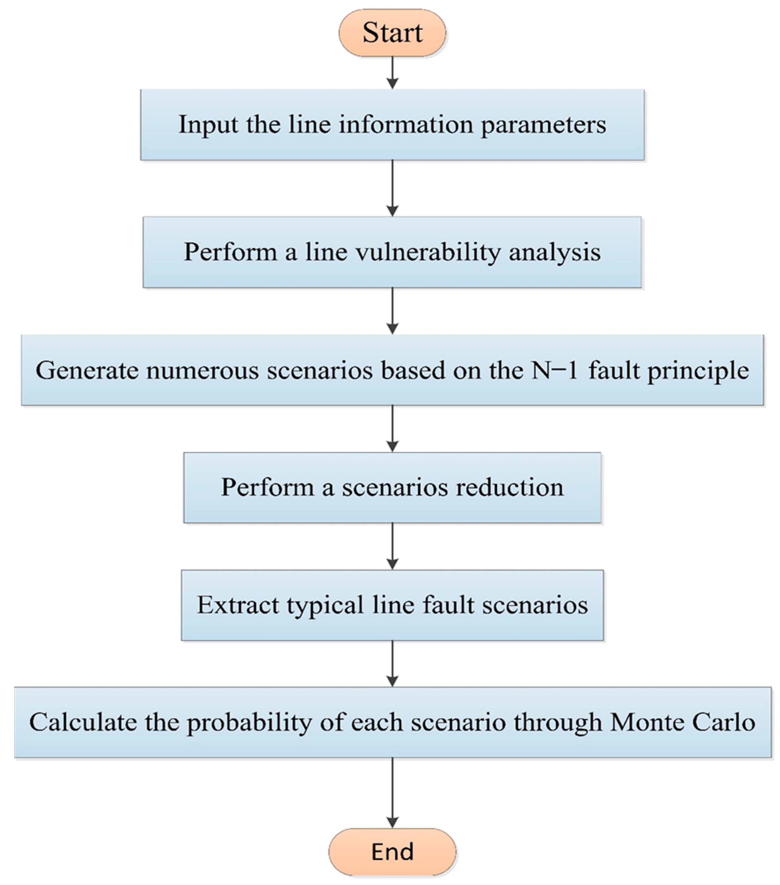
4. Extreme Scenarios
5. Case Studies
5.1. Case Explanation
5.2. Results and Analysis
5.2.1. Power Supply Recovery in Extreme Scenarios
5.2.2. Optimization Results and Economic Analysis
5.2.3. Analysis of the MESS Dispatching Results
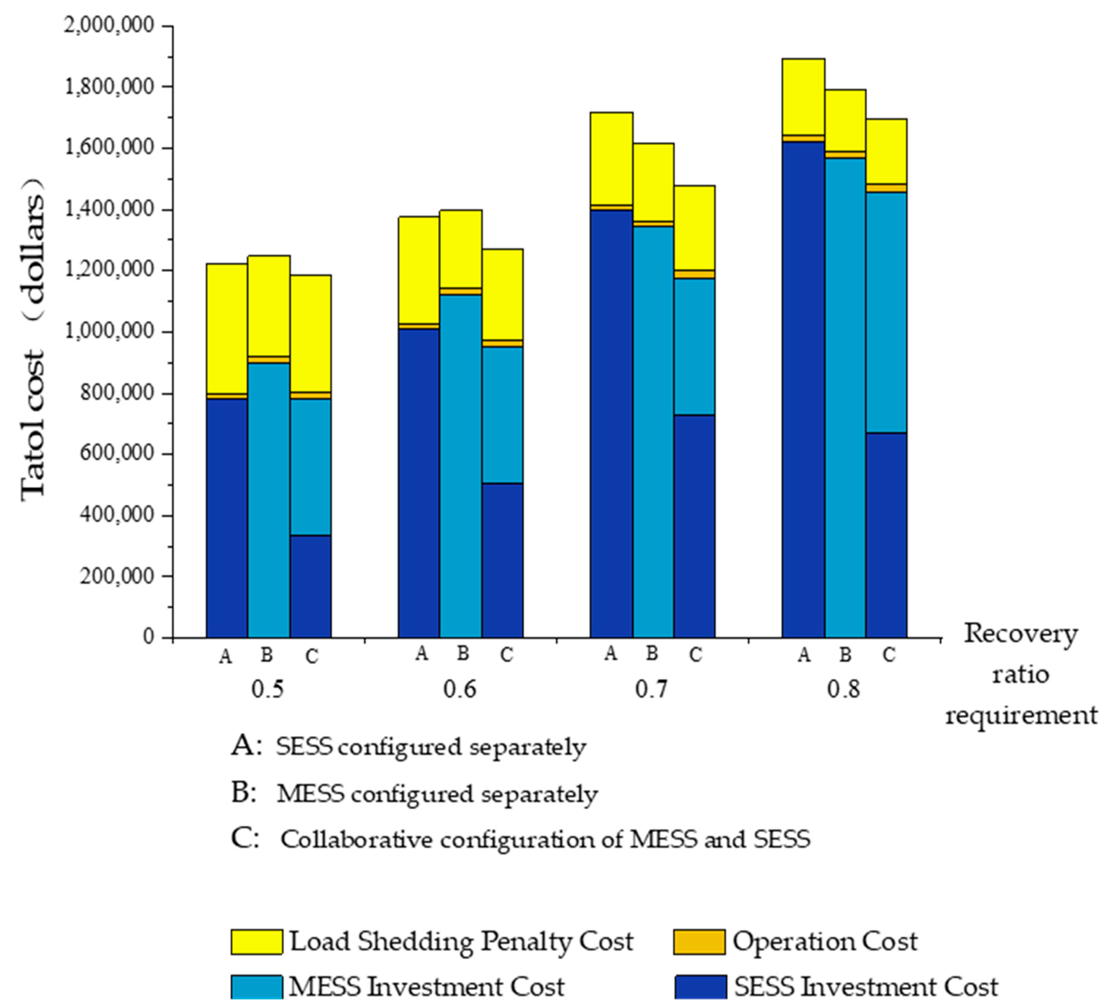
5.2.4. Sensitivity Analysis
6. Conclusions
6.1. Summary
- The collaborative configuration method of two kinds of energy storage system coexistence proposed in this paper combines the time–space characteristics of MESS units and the economic advantage of SESS units. While ensuring reliability and considering economic factors, this system minimizes the total cost.
- The resilience recovery constraint proposed in this paper ensures that the optimization results of the configured energy storage system prioritize power supply reliability in the power system.
- The scenario analysis method is used to address the randomness in the generation of fault scenarios, ensuring that the results of the energy storage system configuration can be applied in various scenarios and that the power support capabilities of the energy storage system are optimal.
6.2. Future Work
Author Contributions
Funding
Data Availability Statement
Conflicts of Interest
Appendix A
References
- Zhang, G.; Zhong, H.; Tan, Z.; Cheng, T.; Xia, Q.; Kang, C. Texas electric power crisis of 2021 warns of a new blackout mechanism. CSEE J. Power Energy Syst. 2022, 8, 1–9. [Google Scholar]
- Hou, H.; Yu, S.; Wang, H.; Huang, Y.; Wu, H.; Xu, Y.; Li, X.; Geng, H. Risk Assessment and Its Visualization of Power Tower under Typhoon Disaster Based on Machine Learning Algorithms. Energies 2019, 12, 205. [Google Scholar] [CrossRef]
- Wang, Y.; Chen, C.; Wang, J.; Baldick, R. Research on Resilience of Power Systems Under Natural Disasters—A Review. IEEE Trans. Power Syst. 2016, 31, 1604–1613. [Google Scholar] [CrossRef]
- Amani, A.M.; Jalili, M. Power Grids as Complex Networks: Resilience and Reliability Analysis. IEEE Access 2021, 9, 119010–119031. [Google Scholar] [CrossRef]
- Wang, Y.; Xu, Y.; He, J.; Liu, C.-C.; Schneider, K.P.; Hong, M.; Ton, D.T. Coordinating Multiple Sources for Service Restoration to Enhance Resilience of Distribution Systems. IEEE Trans. Smart Grid 2019, 10, 5781–5793. [Google Scholar] [CrossRef]
- Nazemi, M.; Moeini-Aghtaie, M.; Fotuhi-Firuzabad, M.; Dehghanian, P. Energy Storage Planning for Enhanced Resilience of Power Distribution Networks Against Earthquakes. IEEE Trans. Sustain. Energy 2020, 11, 795–806. [Google Scholar] [CrossRef]
- Yuan, W.; Wang, J.; Qiu, F.; Chen, C.; Kang, C.; Zeng, B. Robust Optimization-Based Resilient Distribution Network Planning Against Natural Disasters. IEEE Trans. Smart Grid 2016, 7, 2817–2826. [Google Scholar] [CrossRef]
- Ma, S.; Chen, B.; Wang, Z. Resilience Enhancement Strategy for Distribution Systems Under Extreme Weather Events. IEEE Trans. Smart Grid 2018, 9, 1442–1451. [Google Scholar] [CrossRef]
- Yao, S.; Wang, P.; Liu, X.; Zhang, H.; Zhao, T. Rolling Optimization of Mobile Energy Storage Fleets for Resilient Service Restoration. IEEE Trans. Smart Grid 2020, 11, 1030–1043. [Google Scholar] [CrossRef]
- Kim, J.; Dvorkin, Y. Enhancing Distribution System Resilience with Mobile Energy Storage and Microgrids. IEEE Trans. Smart Grid 2019, 10, 4996–5006. [Google Scholar] [CrossRef]
- Yao, S.; Wang, P.; Zhao, T. Transportable Energy Storage for More Resilient Distribution Systems with Multiple Microgrids. IEEE Trans. Smart Grid 2019, 10, 3331–3341. [Google Scholar] [CrossRef]
- Chen, Y.; Zheng, Y.; Luo, F.; Wen, J.; Xu, Z. Reliability Evaluation of Distribution Systems with Mobile Energy Storage Systems. IET Renew. Power Gener. 2016, 10, 1562–1569. [Google Scholar] [CrossRef]
- Teng, F.; Ding, Z.; Hu, Z.; Sarikprueck, P. Technical Review on Advanced Approaches for Electric Vehicle Charging Demand Management, Part I: Applications in Electric Power Market and Renewable Energy Integration. IEEE Trans. Ind. Appl. 2020, 56, 5684–5694. [Google Scholar] [CrossRef]
- Tang, P.; Wang, C.; Jiang, B. A Proximal-Proximal Majorization-Minimization Algorithm for Nonconvex Rank Regression Problems. IEEE Trans. Signal Process. 2023, 71, 3502–3517. [Google Scholar] [CrossRef]
- Shen, J.; Kammara, E.K.H.; Du, L. Nonconvex, Fully Distributed Optimization Based CAV Platooning Control Under Nonlinear Vehicle Dynamics. IEEE Trans. Intell. Transport. Syst. 2022, 23, 20506–20521. [Google Scholar] [CrossRef]
- Jiang, X.; Chen, J.; Wu, Q.; Zhang, W.; Zhang, Y.; Liu, J. Two-Step Optimal Allocation of Stationary and Mobile Energy Storage Systems in Resilient Distribution Networks. J. Mod. Power Syst. Clean Energy 2021, 9, 788–799. [Google Scholar] [CrossRef]
- Zhao, Q.; Du, Y.; Zhang, T.; Zhang, W. Resilience Index System and Comprehensive Assessment Method for Distribution Network Considering Multi-Energy Coordination. Int. J. Electr. Power Energy Syst. 2021, 133, 107211. [Google Scholar] [CrossRef]
- Chen, C.; Wang, J.; Qiu, F.; Zhao, D. Resilient Distribution System by Microgrids Formation After Natural Disasters. IEEE Trans. Smart Grid 2016, 7, 958–966. [Google Scholar] [CrossRef]
- Ouyang, M.; Dueñas-Osorio, L.; Min, X. A Three-Stage Resilience Analysis Framework for Urban Infrastructure Systems. Struct. Saf. 2012, 36–37, 23–31. [Google Scholar] [CrossRef]
- Lin, Y.; Bie, Z. Tri-Level Optimal Hardening Plan for a Resilient Distribution System Considering Reconfiguration and DG Islanding. Appl. Energy 2018, 210, 1266–1279. [Google Scholar] [CrossRef]
- Faqiry, M.N.; Edmonds, L.; Zhang, H.; Khodaei, A.; Wu, H. Transactive-Market-Based Operation of Distributed Electrical Energy Storage with Grid Constraints. Energies 2017, 10, 1891. [Google Scholar] [CrossRef]
- Panteli, M.; Pickering, C.; Wilkinson, S.; Dawson, R.; Mancarella, P. Power System Resilience to Extreme Weather: Fragility Modeling, Probabilistic Impact Assessment, and Adaptation Measures. IEEE Trans. Power Syst. 2017, 32, 3747–3757. [Google Scholar] [CrossRef]
- Wang, Y.; Zhong, H.; Xia, Q.; Kirschen, D.S.; Kang, C. An Approach for Integrated Generation and Transmission Maintenance Scheduling Considering N-1 Contingencies. IEEE Trans. Power Syst. 2016, 31, 2225–2233. [Google Scholar] [CrossRef]
- Taheri, B.; Safdarian, A.; Moeini-Aghtaie, M.; Lehtonen, M. Distribution System Resilience Enhancement via Mobile Emergency Generators. IEEE Trans. Power Deliv. 2021, 36, 2308–2319. [Google Scholar] [CrossRef]
- Zheng, X.; Qu, K.; Lv, J.; Li, Z.; Zeng, B. Addressing the Conditional and Correlated Wind Power Forecast Errors in Unit Commitment by Distributionally Robust Optimization. IEEE Trans. Sustain. Energy 2021, 12, 944–954. [Google Scholar] [CrossRef]
- Lu, Y.; Xiang, Y.; Huang, Y.; Yu, B.; Weng, L.; Liu, J. Deep Reinforcement Learning Based Optimal Scheduling of Active Distribution System Considering Distributed Generation, Energy Storage and Flexible Load. Energy 2023, 271, 127087. [Google Scholar] [CrossRef]
- Li, Y.; Feng, B.; Li, G.; Qi, J.; Zhao, D.; Mu, Y. Optimal Distributed Generation Planning in Active Distribution Networks Considering Integration of Energy Storage. Appl. Energy 2018, 210, 1073–1081. [Google Scholar] [CrossRef]
- Zhang, J.; Zhu, L.; Zhao, S.; Yan, J.; Lv, L. Optimal Configuration of Energy Storage Systems in High PV Penetrating Distribution Network. Energies 2023, 16, 2168. [Google Scholar] [CrossRef]
- Guo, F.; Li, J.; Zhang, C.; Zhu, Y.; Yu, C.; Wang, Q.; Buja, G. Optimized Power and Capacity Configuration Strategy of a Grid-Side Energy Storage System for Peak Regulation. Energies 2023, 16, 5644. [Google Scholar] [CrossRef]
- Wu, Y.-K.; Chen, Y.-C.; Chang, H.-L.; Hong, J.-S. The Effect of Decision Analysis on Power System Resilience and Economic Value During a Severe Weather Event. IEEE Trans. Ind. Appl. 2022, 58, 1685–1695. [Google Scholar] [CrossRef]
- Wang, Y.; Huang, L.; Shahidehpour, M.; Lai, L.L.; Zhou, Y. Impact of Cascading and Common-Cause Outages on Resilience-Constrained Optimal Economic Operation of Power Systems. IEEE Trans. Smart Grid 2020, 11, 590–601. [Google Scholar] [CrossRef]

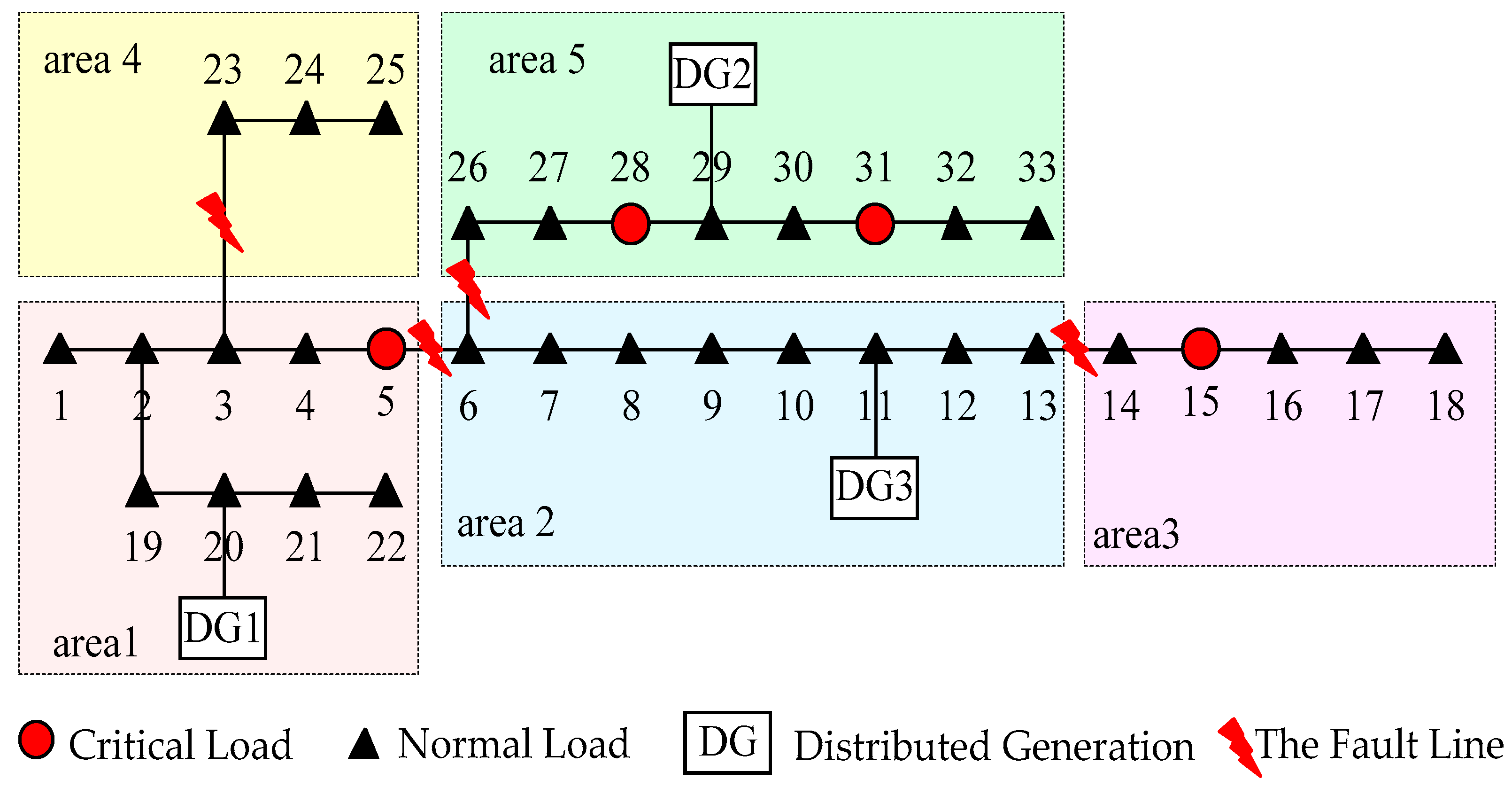
| Scenario Number | Fault Line | Power Loss Area | Scenario Probability |
|---|---|---|---|
| 1 | 5–6 | 2, 3, 5 | 0.213 |
| 2 | 13–14 | 3 | 0.204 |
| 3 | 3–23 | 4 | 0.305 |
| 4 | 6–26 | 5 | 0.278 |
| Case | SESS Investment Cost (Dollars) | MESS Investment Cost (Dollars) | Operational Cost (Dollars) | Load Shedding Penalty Cost (Dollars) | Total Cost (Dollars) |
|---|---|---|---|---|---|
| 1 | \ | \ | 15,470 | 1,265,068 | 1,280,538 |
| 2 | 784,000 | \ | 16,086 | 434,994 | 1,235,094 |
| 3 | \ | 896,000 | 23,905 | 325,192 | 1,246,042 |
| 4 | 336,000 | 448,000 | 20,412 | 397,152 | 1,201,564 |
| Case | SESS Results (Configured Node × Number of Configurations) | MESS Results (Configured Node × Number of Configurations) | Total Configured Capacity /kW·h |
|---|---|---|---|
| 1 | \ | \ | \ |
| 2 | 14 × 4, 16 × 1, 23 × 2, 26 × 5, 31 × 2 | \ | 5600 |
| 3 | \ | 5 × 4 | 3200 |
| 4 | 14 × 2, 28 × 3, 31 × 1 | 5 × 2 | 4000 |
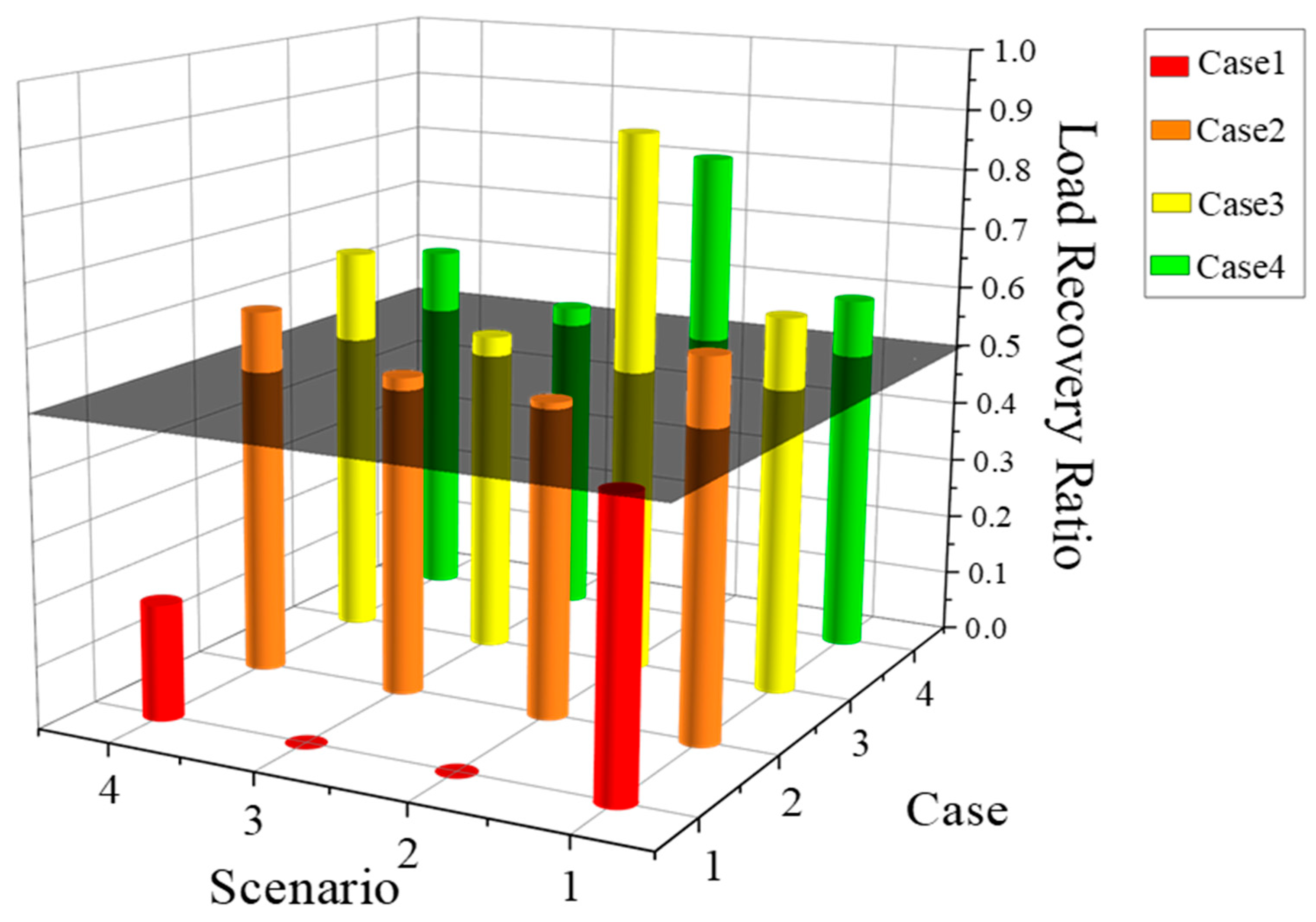
| Case | Critical Load Recovery Ratio | Normal Load Recovery Ratio |
|---|---|---|
| 1 | 79.28% | 40.66% |
| 2 | 100% | 54.17% |
| 3 | 100% | 59.63% |
| 4 | 100% | 56.48% |
Disclaimer/Publisher’s Note: The statements, opinions and data contained in all publications are solely those of the individual author(s) and contributor(s) and not of MDPI and/or the editor(s). MDPI and/or the editor(s) disclaim responsibility for any injury to people or property resulting from any ideas, methods, instructions or products referred to in the content. |
© 2023 by the authors. Licensee MDPI, Basel, Switzerland. This article is an open access article distributed under the terms and conditions of the Creative Commons Attribution (CC BY) license (https://creativecommons.org/licenses/by/4.0/).
Share and Cite
Zhou, W.; Zhao, P.; Lu, Y. Collaborative Optimal Configuration of a Mobile Energy Storage System and a Stationary Energy Storage System to Cope with Regional Grid Blackouts in Extreme Scenarios. Energies 2023, 16, 7903. https://doi.org/10.3390/en16237903
Zhou W, Zhao P, Lu Y. Collaborative Optimal Configuration of a Mobile Energy Storage System and a Stationary Energy Storage System to Cope with Regional Grid Blackouts in Extreme Scenarios. Energies. 2023; 16(23):7903. https://doi.org/10.3390/en16237903
Chicago/Turabian StyleZhou, Weicheng, Ping Zhao, and Yifei Lu. 2023. "Collaborative Optimal Configuration of a Mobile Energy Storage System and a Stationary Energy Storage System to Cope with Regional Grid Blackouts in Extreme Scenarios" Energies 16, no. 23: 7903. https://doi.org/10.3390/en16237903
APA StyleZhou, W., Zhao, P., & Lu, Y. (2023). Collaborative Optimal Configuration of a Mobile Energy Storage System and a Stationary Energy Storage System to Cope with Regional Grid Blackouts in Extreme Scenarios. Energies, 16(23), 7903. https://doi.org/10.3390/en16237903