Refining the Selection of Historical Period in Analog Ensemble Technique

Abstract

A precise estimate of solar energy output is essential for its efficient integration into the power grid as solar energy becomes a more significant renewable energy source. Contrarily, the creation of solar energy involves fluctuation and uncertainty. The integration and operation of energy systems are complicated by the uncertainty in solar energy projection. As a post-processing technique to lower systematic and random errors in the operational meteorological forecast model, the analog ensemble algorithm will be introduced in this study. When determining the appropriate historical and predictive data required to use the approach, an optimization is conducted for the historical period in order to further maximize the capabilities of the analog ensemble. To determine statistical consistency and spread skill, the model is evaluated against both the raw forecast model and observations. The outcome lowers the uncertainty in the predicted data by demonstrating that statistical findings improve significantly even with 1-month historical data. Nevertheless, the optimization with a year’s worth of historical data demonstrates a notable decrease in the outcomes, limiting overestimation and lowering uncertainty. Specifically, analog ensemble algorithms calibrate analog forecasts that are equivalent to the latest target forecasts within a set of previous deterministic forecasts. Overall, we conclude that analog ensembles assuming a 1-year historical period offer a comprehensive method to minimizing uncertainty and that they should be carefully assessed given the specific forecasting aims and limits.

1. Introduction

The operational meteorological forecast (OMF) model has been primarily used in solar power prediction as well as weather forecasts. This model is essential for day-to-day solar resource assessment and further for the long-term climate outlook [1]. Variables such as surface temperature, pressure, solar irradiance taken from OMF are employed to estimate the amount of solar power that will be generated at a specific location over a defined period of time. OMF exhibits a reliable wind and solar forecast up to three days ahead, although there are still uncertainties to consider [2]. The accuracy of OMF is consequential in electricity generation and in electricity trading. For example, in a hybrid system, forecasting is important in determining the energy mix and preventing disruption by providing traditional energy sources such as hydrothermal, gas, or coal as back-up sources [3,4]. In some countries, power producers are penalized if they do not deliver the committed energy production amounts. OMF has also been used to evaluate and assess the overall performance of renewable power plants.

The integration of solar energy forecasting is not only vital for ensuring the stability and optimal functioning of solar power plants but also holds significant implications for the diverse energy landscape of residential buildings. While residential structures constitute approximately 25% of the total final energy consumption [5], their energy needs exhibit a broad spectrum, surpassing the range observed in commercial and industrial counterparts. As highlighted in the 2021 Global Status Report for Building and Construction [6], the overall building sector accounted for a substantial 37% of total energy consumption, encompassing both operational and process-related aspects [7]. Solar forecasting, traditionally associated with energy producers, extends its relevance to various building types, including the paradigm of autonomous buildings or smart structures capable of operating independently from external infrastructural support like electric power [8]. For autonomous buildings, renewable energy stands as the undisputed priority, with solar forecasting emerging as a crucial tool in mitigating challenges posed by occupancy patterns that contribute to fluctuating energy demands throughout consumption periods. Despite the myriad of benefits attributed to solar forecasting, it is imperative to acknowledge inherent limitations.

One of the limitations in solar forecasting is the uncertainty of weather forecast itself [9]. Solar forecasting heavily relies on weather prediction models, which can be complex, especially in long-term forecasts. These are caused by rapid changes in atmospheric conditions and other weather phenomena that can impact radiation levels. Spatial variability is another factor [10]. Irradiance can sometimes vary significantly within a relatively small area, factors such as topography, shadowing, and other factors that cause spatial variation in solar energy prediction. Another limitation is the forecast horizon [11], long forecast horizon deprives solar predictability. Finally, the solar forecasting model may struggle to account for sudden operational changes or unexpected events that can affect solar energy generation [12].

Despite several limitations, solar forecasting has made significant contributions to energy resource harvesting and allocation. Thus, to improve the reliability and dependability of solar forecasting, post-processing techniques are introduced [13,14,15]. While solar forecasting involves predicting the amount of solar energy that will be generated, post-processing techniques are used to increase the accuracy [16] of solar forecasts by refining raw forecast data. Post-processing techniques help refine the initial forecast, which is vital for efficient integration of solar energy into the grid and optimizing grid operation [17]. One of the techniques used is ensemble forecasting. Ensemble forecasting involves generating multiple forecasts using different models or variations in the input data. Ensembles are then combined to create an ensemble forecast, which can provide a more reliable prediction. Analog ensemble is one of the ensemble forecast techniques used in solar forecasting [18].

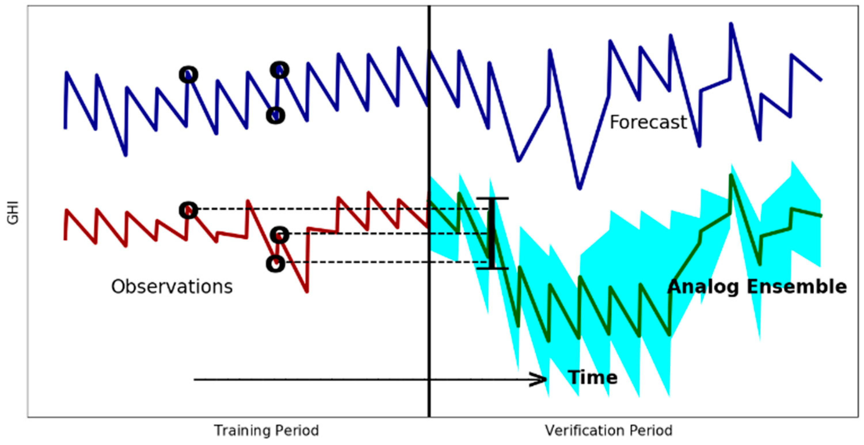
Analog ensemble forecasting in solar forecasting refers to techniques that use historical analogs or similar patterns in solar radiation data to improve the accuracy and reliability of solar energy generation predictions [19,20]. The analog ensemble technique leverages the idea that similar atmospheric patterns tend to produce similar weather outcomes. By identifying historical situations that closely resemble the current condition, the technique aims to capture the likely ranges of outcomes for the forecasted variable, such as the solar irradiance.

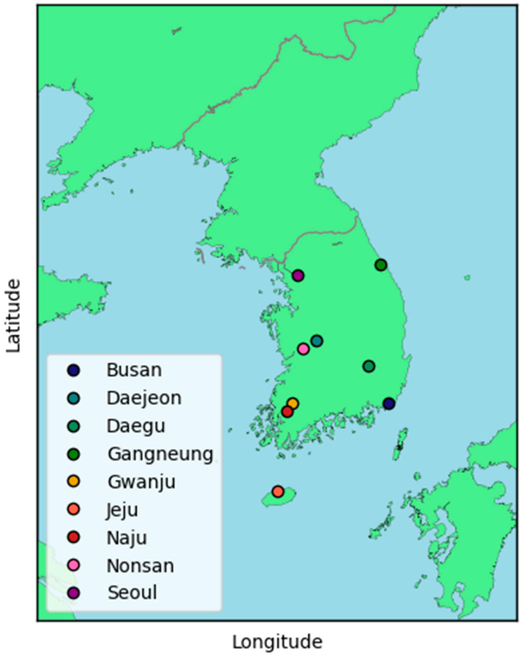
The goal of this paper is to create and put into use an analog ensemble prediction system that is appropriate for a weather forecast model operated by the Korea Meteorological Administration (KMA). Additionally, in this research, historical period optimization will be used to further maximize the analog ensemble’s capabilities. By identifying the most suitable dynamic period for observations through careful evaluation and cross-validation, analog ensemble forecasts can provide valuable insights for decision-making across various domains, ranging from weather and climate predictions to resource management and risk assessment. This will increase the precision and dependability of future forecasts by utilizing the knowledge and data from past occurrences. The operational meteorological forecast model’s integration of analog ensemble forecasts will be examined for its calibration through statistical validation.

2. Materials and Methods

2.1. Data

The observed solar irradiance data of global horizontal irradiance (GHI) and direct normal irradiance (DNI) were derived by the University of Arizona Solar Irradiance Based on Satellite-Korea Institute of Energy Research (UASIBS-KIER) model [21] over a two-year period from January 2018 to December 2019. This study-prescribed history dataset for analog ensemble prediction relied on the dynamic period selection, starting from a month of historical data and growing by a month until they reach a full year (see Figure 1. OMF came from Unified Model Local Data Assimilation and Prediction System (UMLDAPS), which was initialized at 03 Korean Standard Time (KST) from January 2018 to December 2019. As the solar irradiance forecast here was performed for a same-day forecast, model outputs were valid for a span between 06 and 20 KST, which corresponded to forecast horizons of 03 and 17 h, respectively. Vanyyye et al. [22] pointed out that the utilization of 365 days was adequate as the history datasets of previous observations. That is why this study also limits the historical data to reaching a full year. Figure 2 illustrates the geographical locations of ground observing stations in Korea; Busan (35.17° N, 129.07° E), Daejeon (36.35° N, 127.39° E), Daegu (35.87° N, 128.59° E), Gangneung (37.75° N, 128.87° E), Gwangju (35.17° N, 126.85° E), Jeju (33.51° N, 126.52° E), Naju (35.03° N, 126.72° E), Nonsan (36.2° E, 127.08° N), and Seoul (37.53° N, 127.02° E).

2.2. Analog Ensemble Prediction

Analog ensemble prediction (AnEn) is usually classified into the post-processing of forecast data that utilizes historical analogs to make predictions about future events or conditions. It is based on the concept that similar patterns in the past tend to be associated with similar outcomes in the future, and its equation [23,24] is defined as follows:

$$\Vert F_t,A_t\Vert ={{\displaystyle \sum }}_{i=1}^{N_v}\frac{w_i}{{\sigma }_{fi}}\sqrt{{{\displaystyle \sum }}_{j=-k}^k{(F_{i,t-j}-A_{i,t+j})}^2},$$

(1)

where F_t is the current numerical deterministic forecast at future t; A_t is the analog forecast at the same time and location valid at past time t’; N_v is the number of physical variables, whereas w_i is the weight of each variable; σ_fi is the standard deviation of the training time series; and k is the half of the number of additional times computed. The use of the equation requires at least two variables (w_i), and this study selects GHI and DNI with equal weights [25,26]. Here, F_t is taken from UM-LDAPS model’s corresponding weights, and A_t is historical data from satellite-derived solar irradiance produced by the UASIBS-KIER model. Finally, compute the analog ensemble forecast by computing the distance of every lead from past forecasts issued at the same time by using Equation (1). The prediction is calculated based on independent searches. Arrange the data and select the 20 best forecasts by using the error distance. Find the average value from the selected analogs, and this will constitute the analog ensemble forecast for the same historical period and location. These steps provide a significant result since it will not have a cumulative error, and there are no missing predictions.

2.3. Statistical Forecast Evaluation

Statistical evaluation for AnEn involves assessing the performance and skill of the ensemble forecast generated using the analog ensemble method. In this study, several error statistics are used for the verification of the AnEn and its effectiveness compared to OMF. Correlation coefficient, Mean Bias Error (MBE), Mean Absolute Error (MAE), Root Mean Square Error (RMSE), and Skill score are employed here as error statistics.

$$MBE=\frac{1}{N}{\displaystyle \sum _{i=1}^N\left(y_p^i-y_o^i\right)}$$

(2)

$$MAE=\frac{1}{N}{\displaystyle \sum _{i=1}^N\left(\left|y_p^i-y_o^i\right|\right)}$$

(3)

$$RMSE=\sqrt{\frac{1}{N}{{\displaystyle \sum _{i=1}^N\left(y_p^i-y_o^i\right)}}^2}$$

(4)

$$\mathrm{Skill} \mathrm{Score} =\frac{MA{E}_{OMF}-MA{E}_{AN}}{MA{E}_{OMF}}$$

(5)

Above, y_p, y_o, and N indicate the forecast, observation, and number of samples, respectively. Furthermore, Skill score represents the improvement of AnEn in comparison with OMF.

3. Results

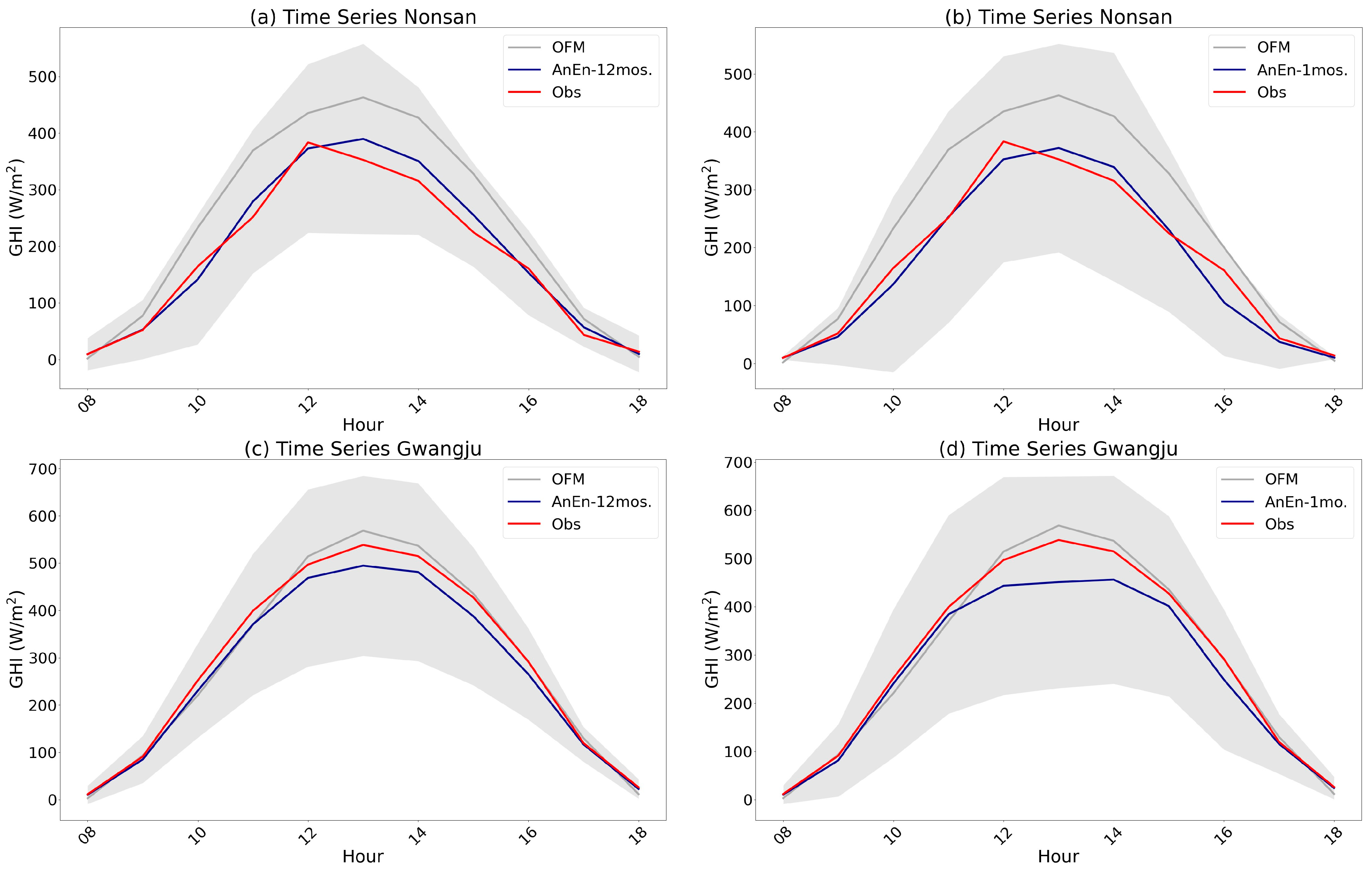
Two examples are given in Figure 3, which shows the time series of solar irradiance forecast from OMF and AnEn that is produced by 12 months dataset and a month dataset with observation data at Nonsan and Gwangju stations. As AnEn is one of probabilistic forecast, prediction interval at 95% confidence level is also illustrated in Figure 3. In the context of Nonsan station’s historical data analysis, spanning both a concise one-month period and a more comprehensive twelve-month duration, a noteworthy observation emerges. Specifically, during the hours between 12 to 16 KST, the OMF exhibits a propensity to deviate from actual observations. However, this deviation was not left unaddressed. Through the application of an analog ensemble approach, a method renowned for its proficiency in harnessing historical precedents, the previously mentioned discrepancy in the OMF’s predictions was adeptly compensated and rectified. This intriguing occurrence prompts a nuanced discussion about the efficacy of analog ensembles in improving model deviations, especially within the temporal framework of midday to late afternoon, and the potential implications of such compensation on enhancing the overall accuracy and reliability of operational meteorological forecasts at Nonsan station. When using 12-month historical data, the AnEn’s prediction interval is more condensed than when using 1-month historical data. The result comparing 1 month to 12 months gradually increased, with the prediction interval decreasing every 1 month increment in the dynamic period of observation data. This shows that there are few deviations from the observed data and a higher level of confidence in the model’s predictions. As the AnEn similarly confronts the outcome of the observed data, the pattern and observation of the result are also comparable to those at the Gwangju station (see Figure 3c,d). When compared to AnEn with a 1-month historical period in Gwangju, AnEn with 12-month historical data also provided a narrow predicted interval, demonstrating minimal uncertainty and showing a significant agreement with the observed value.

Table 1. Summary of Average of observation data, error statistics of OMF and AnEn.

Station	Average			OMF				AnEn
	Obs	OMF	AnEn	Corr.	MBE	MAE	RMSE	Corr.	MBE	MAE	RSME	Skill Score (%)
Busan	336.84	393.15	334.34	0.9372	56.31	49.54	105.46	0.9807	−2.5	22.23	50.48	52.13
Daegu	326.26	374.66	328.22	0.9401	48.40	44.82	97.69	0.9806	1.95	21.21	48.63	50.22
Daejeon	320.21	375.92	322.34	0.9368	55.71	46.59	102.01	0.9829	2.14	19.68	44.85	56.03
Gangneung	305.27	356.99	307.60	0.9263	51.72	46.88	104.16	0.9766	2.33	23.42	51.47	50.58
Gwanju	317.23	372.29	322.38	0.9378	55.06	46.18	100.64	0.9835	5.14	19.49	44.02	56.26
Jeju	303.89	371.68	301.50	0.9156	67.79	55.35	117.47	0.9805	−2.4	22.52	48.65	58.58
Naju	320.74	374.91	322.52	0.9374	54.17	46.41	100.70	0.9829	1.78	20.13	45.29	55.03
Nonsan	322.93	373.30	321.30	0.9414	50.37	44.66	97.12	0.9840	−1.63	19.63	44.07	54.63
Seoul	317.01	377.41	314.74	0.9393	60.40	46.14	102.29	0.9783	−2.27	22.80	50.36	50.77
TOTAL	318.93	374.48	319.44	0.9348	55.55	47.04	103.06	0.9811	0.51	21.23	47.54	53.80

displays the average of the observations in comparison to the OMF and AnEn operated by 12 months datasets. Although OMF indicated great performance with an average correlation value of 0.9348 and a high degree of linear association, the correlation increased to 0.9811 on average with the deployment of the analog ensemble. There is a strong positive bias, with results ranging from 48 to 67 W/m² per station, demonstrating that the OMF routinely overestimates the observed values, which was greatly reduced, indicating that it is generally less biased in its predictions than the OMF. Further examination of mean absolute error (MAE) and root mean square error (RMSE) confirms the analog ensemble’s superiority. OMF’s MAE and RMSE are around 47.04 and 103.06 W/m², respectively. These values, however, are halved with the introduction of the analog ensemble, suggesting a considerable reduction in prediction errors and a significant improvement in forecast precision on average. The outcomes are represented in its skill score; the reduction in error statistics has also been validated by the skill score, with an average improvement of more than 50% when analog ensemble is used. These findings emphasize the extraordinary development made in forecasting, which promises more precise and dependable predictions for a wide range of applications. The highlighted stations are marked for additional review in the following paragraph.

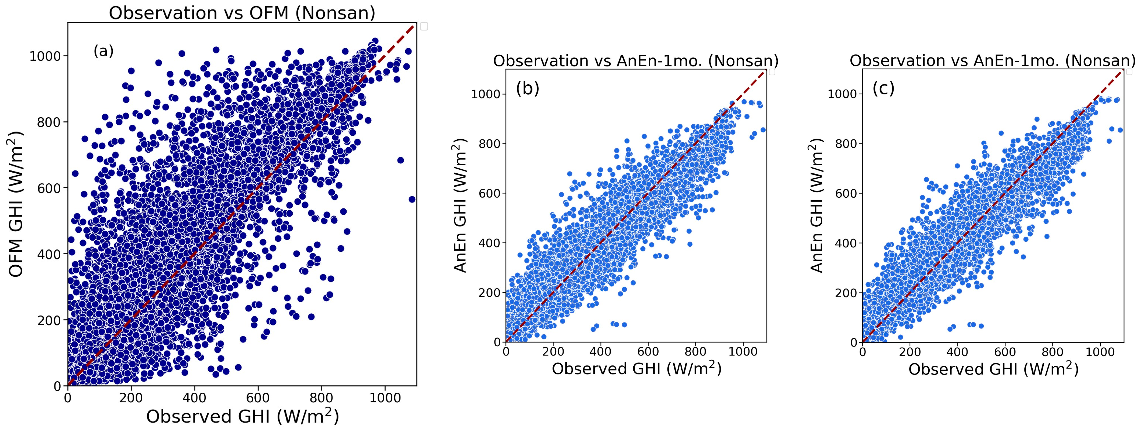
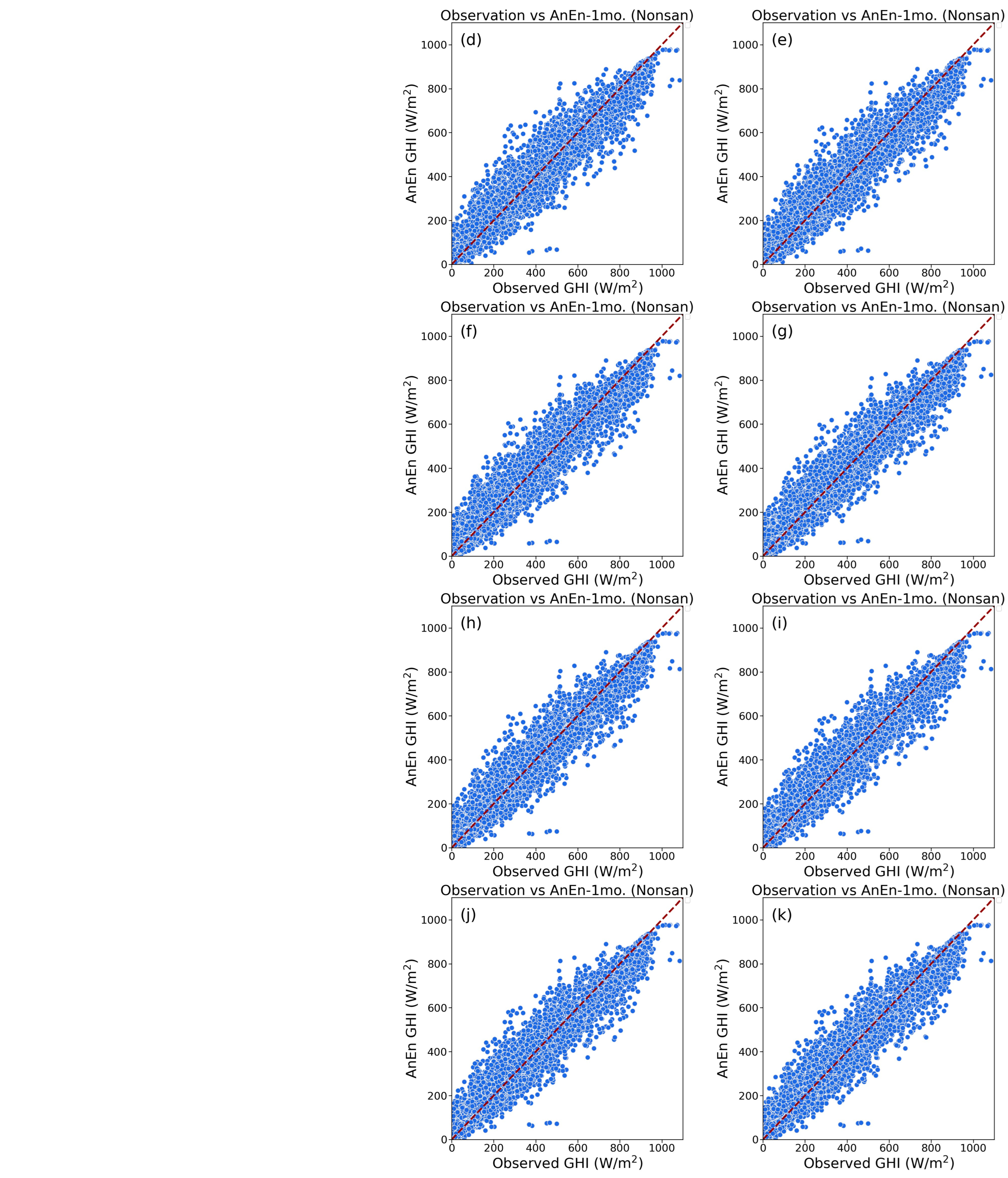
To further evaluate the result, a scatter diagram is used to determine the analog ensemble’s overall performance. Studying the scatter plot (see Figure 4a) demonstrates how OMF overestimates the predicted value since the data are more strongly moved upwards. We can state that the data seems to improve even on a 1-month historical basis when compared to the AnEn vs. observation plots. The close alignment of the data points in the AnEn versus observation data along a diagonal line suggests a linear relationship between the variables. This implies a strong positive correlation between the two variables, indicating that the trends in their values are similar. As a result, we are able to draw conclusions regarding the outcome of the analog ensemble post-processing method. The statistical analysis also shows that the OMF is dispersed with bigger deviations from the reference line as compared to the observation value, indicating considerable discrepancies that lead to lower accuracy. Contrarily, each data point for analog ensembles is densely packed around the reference line, demonstrating agreement between the ensemble’s predictions and the observational results (see Figure 4). This gives us a better understanding of how performing analog ensemble as a post-processing technique for all places detected has improved overall. The scatter plot of the AnEn vs. observations plot generally does not appear to exhibit differences in terms of improvement, so it is important to validate the outcome to statistical verification.

4. Discussion

Delving into the realm of forecast evaluation and the application of analog ensemble, this discussion centers on our assessment of correlation, MAE, RMSE, and bias as benchmarks of model accuracy. By scrutinizing the correlations between predicted and observed values, we gauge the level of association that underpins our forecasts. Simultaneously, we dissect the magnitudes of errors through MAE and RMSE, which together convey the predictive precision. Lastly, we untangle the presence of systematic tendencies via bias analysis. Our synthesis of these metrics provides a holistic understanding of analog ensemble and the right historical periods.

The correlation plot for all stations using the analog ensemble is shown in Figure 5. The analog ensemble result is impacted by the applicability of a long historical period. In the 1-year historical dataset compared to a 1-month historical period, the correlation is highest. A longer historical period will have a positive impact across all stations by as much as 4%. Although the result is noticeably high compared to the ongoing forecast from the OMF. In Table 1 for instance, the correlation between observation data and the Nonsan station of the OMF is 94.14%; however, when the analog ensemble prediction is used, even with a 1-month historical period, the correlation improves by roughly 98.4%, leading to a reduction in uncertainty. The comparison between the 12-month and 1-month periods reveals a narrow margin between their respective outcomes.

The proposition is that employing a 12-month historical period proves to be as efficient as utilizing a 1-month historical period. This assertion is substantiated by the close resemblance in correlation values evident from the graphical representation. As correlation alone is inadequate at determining the ideal historical period for an analog ensemble, we shall look more closely at the other statistical techniques.

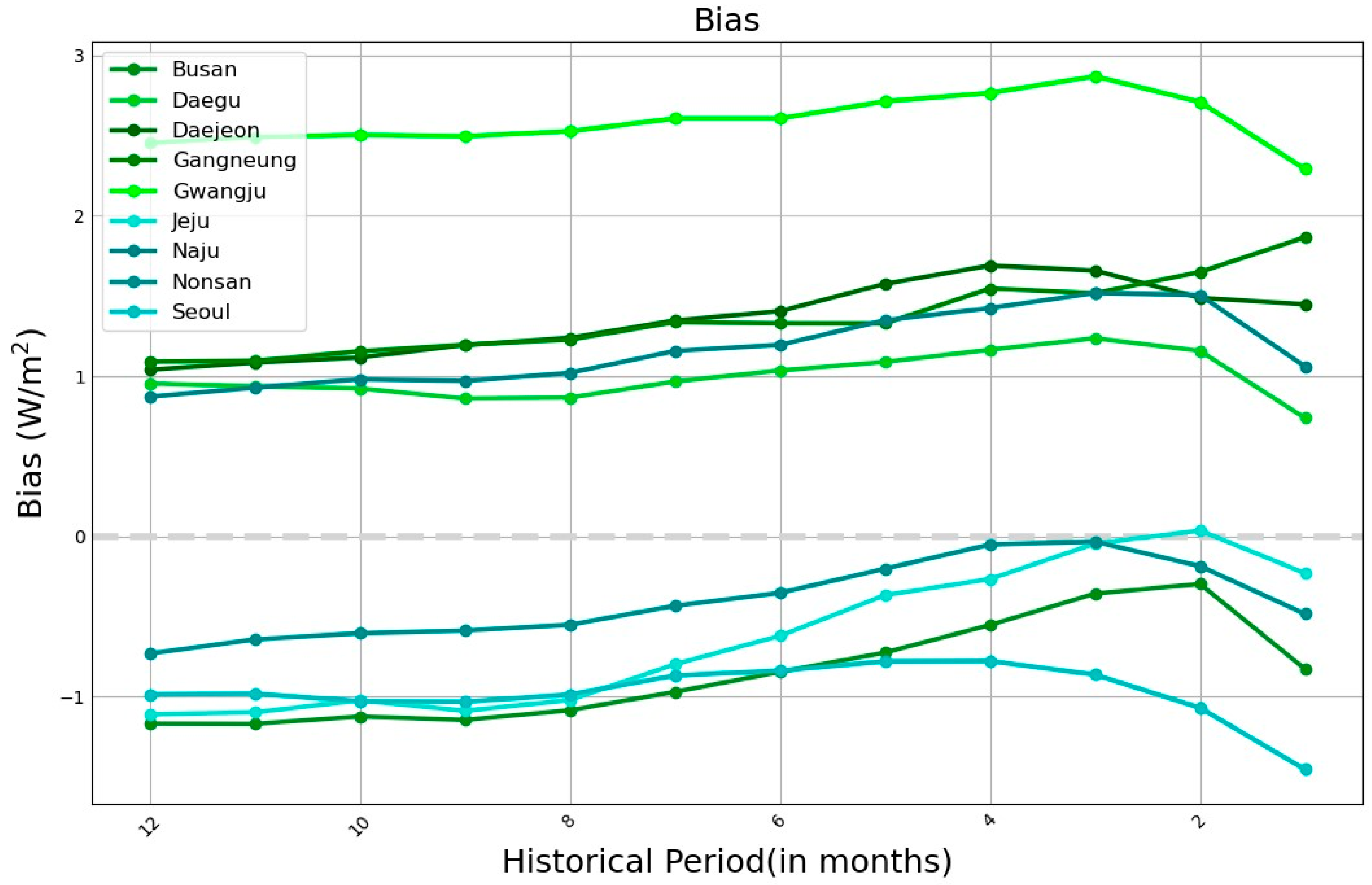
As seen in Figure 6, the bias plot’s distribution is clearly skewed to the right. Except for the Gangneung station, the trend is essentially the same for all of the stations. In comparison to OMF, which ranges from 25.98 to 34.77 W/m², the results for all historical periods are reduced, with the range roughly being −2 to 3 W/m². When the historical period is 3 months, the bias result is the lowest at the other stations, including Busan, Jeju, Naju, and Seoul. However, considering a 1-year historical period, the results are not significantly different from the bias result. Overall, it appears that the analog ensemble method has a smaller bias than OMF based on the bias analysis results. This indicates that the genuine values or consequences have been underestimated. This can be useful in solar PV plants where conservative estimations are required to avoid overestimation and over commitment of resources.

Regarding the performance with respect to historical periods, the analysis indicates a notably reduced bias within the range of 2 to 4 months for certain stations like Busan, Jeju, Nonsan, and Seoul. This finding underscores that forecasts derived from these specific historical windows tend to align more closely with the actual observations, implying a higher accuracy in these cases. Conversely, a reverse trend is observed for other stations, where superior results are achieved when employing a longer historical period. The implication here is that the choice of historical period significantly influences the precision of our forecasts, and station-specific considerations play a pivotal role in determining the optimal historical window. The interaction between historical eras and station features produces complicated dynamics that necessitate careful study for precise forecasts, underscoring the complexity of the forecasting process.

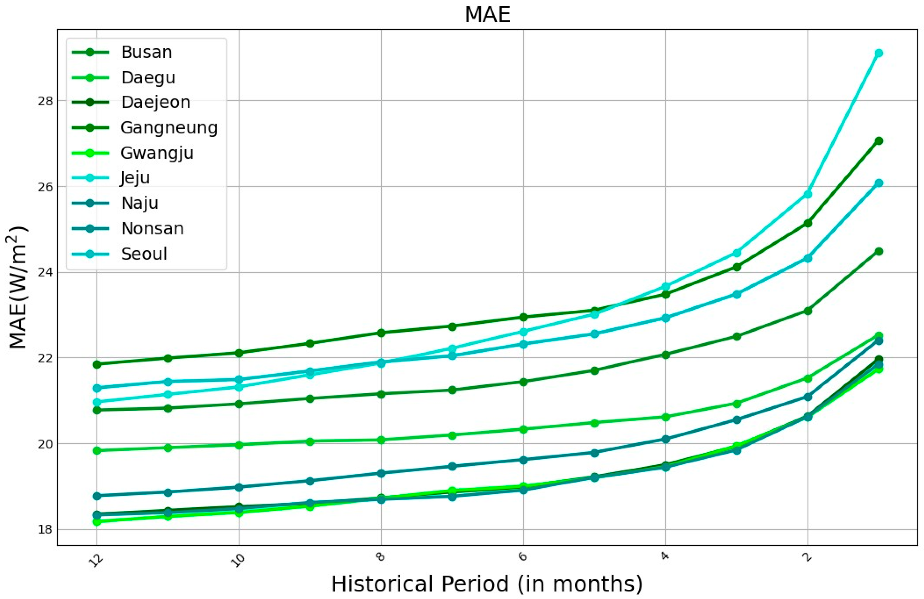
The MAE is cut in half when analog ensemble is applied to OMF’s GHI data. Figure 7 illustrates the considerable decrease in MAE for all locations when compared to OMF. The accuracy and dependability of the forecasting findings are considerably increased by these states. Additionally, if you examine the trend of the analog ensemble at various historical periods, you will notice that all of the plots are comparable and that the AnEn with the 1-year historical period has the lowest MAE, whereas the AnEn with the 1-month historical period has the greatest MAE. On average, the analog ensemble results on historical period of one year are quite near to the actual observed values.

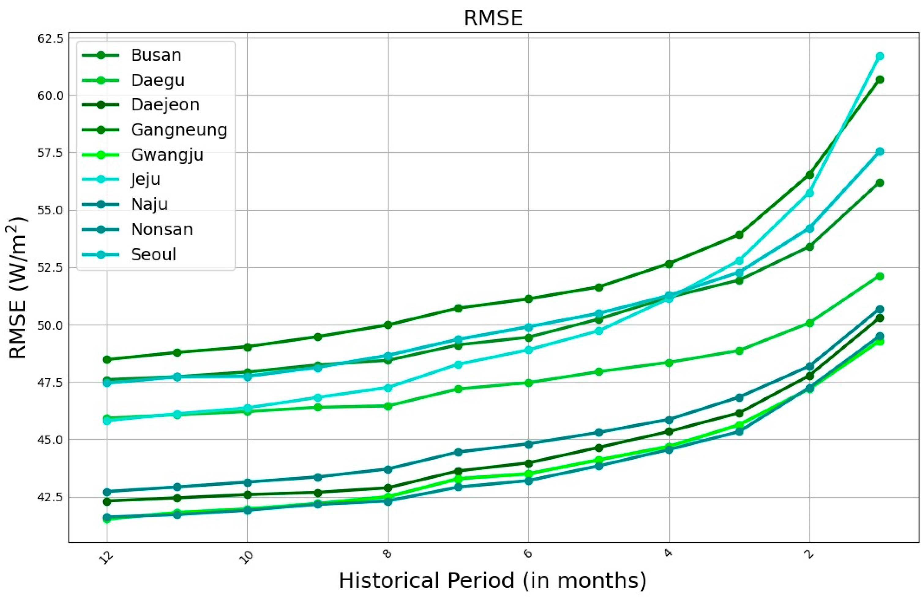
The RMSE plot is the same in Figure 8, which has the same trend as the MAE plot. The RMSE’s output for AnEn at various historical periods is likewise diminished. When compared to OMF, which has RMSE scores between 90 and 100 W/m², AnEn findings range between 40 and 55 W/m² at various historical periods. AnEn exhibits a significant result when compared to OMF on the RSME plot, with a reduction of about 55%. When comparing AnEn results at various historical periods, the 12-month historical period continues to have the lowest RMSE and most dependability.

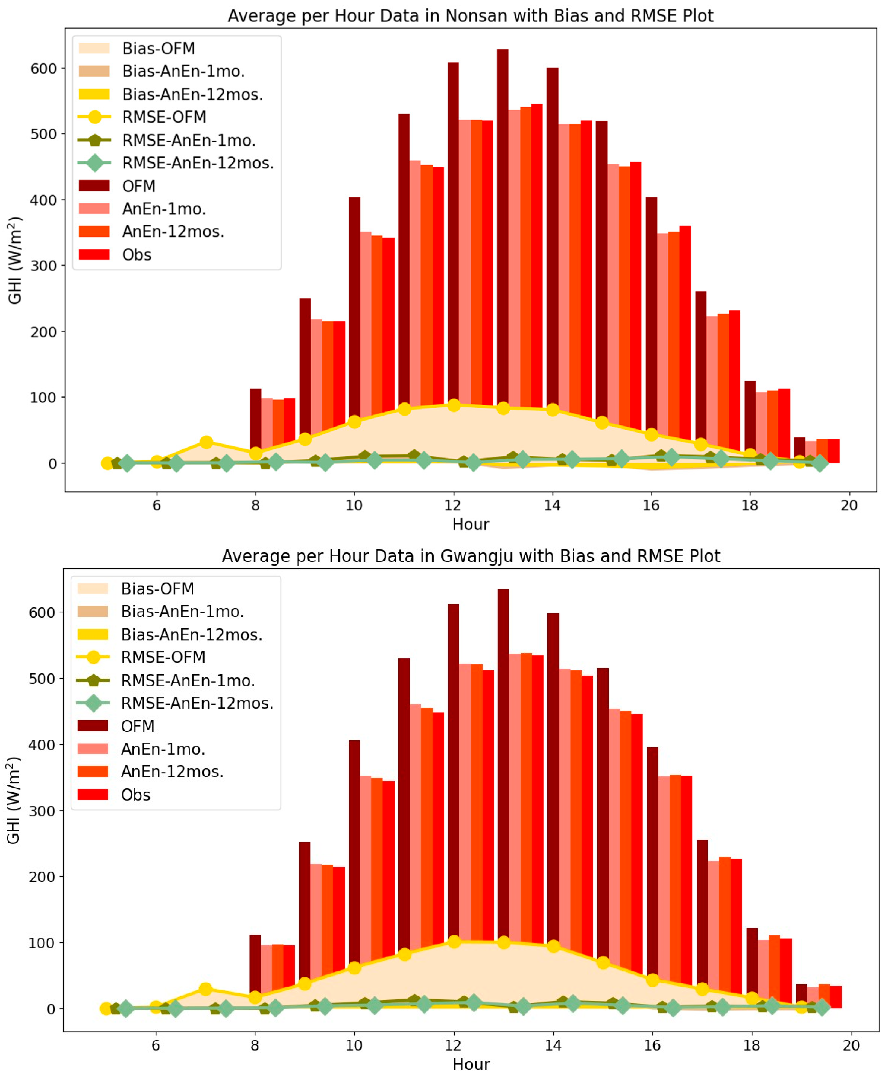
In Figure 9, to determine the analog ensemble forecast, the result needed to identify twenty analog members, as assumed by the researchers. These twenty analog members are derived from the lowest distance from historical patterns. The contribution of the analog members, represented by the dashed lines, defined the mean result of the analog ensemble. The test dataset from the UASIBS-KIER verifies the results of the analog ensemble. The initial 24 h depiction in the figure stands as a notable exemplar. Here, the analog ensemble effectively unfolds a trajectory that closely mirrors the observation data, signifying a commendable alignment between the model’s predictions and the actual occurrences. One noteworthy observation emerges when comparing the root mean square error (RMSE) outcomes. Notably, there exists a proportional relationship between the RMSE values and the biased results in the context of the OMF. Intriguingly, this pattern experiences a significant reduction when the analog ensemble approach is applied. This implies that the analog ensemble method contributes not only to minimizing biases but also to restraining the overall magnitude of errors, effectively elevating the predictive capability of the model. The interplay between bias reduction and RMSE diminishment highlights the synergy between these evaluation metrics and underscores the efficacy of the analog ensemble technique in enhancing forecast precision. In essence, the strategic selection of analog members, coupled with their cumulative impact on forecast generation, underscores the rationale and potential of the analog ensemble approach. Its alignment with observation data, coupled with the advantageous reduction in both biases and errors, accentuates its practicality in improving forecasting accuracy across a diverse range of scenarios. This robust approach encapsulates the fusion of historical patterns and modern computational methodologies, culminating in a predictive framework that holds promise in a variety of forecasting applications.

The average error between the observation value and the OMF/analog ensemble is measured by the RSME value. Analog ensemble reveals that outcomes are more consistent with observation value when RSME is lower. The average overall RSME percentage has been reduced across the board by 74%, demonstrating that analog ensembles improve forecast accuracy (see Figure 9).

While our study provides valuable insights into the application of AnEn in solar irradiance forecasting, it is essential to acknowledge certain limitations. The effectiveness of the analog ensemble method is contingent upon the availability and quality of historical data. Variations in the performance of the analog ensemble across different stations highlight the sensitivity of the approach to regional differences and microclimates. Additionally, the study primarily focuses on specific regions in South Korea, and the applicability of the findings may vary when extrapolated to other geographical locations with distinct weather patterns. Future research endeavors could explore the optimization of the analog ensemble method for different climatic conditions and diverse datasets and optimization of the appropriate analog ensemble members given a one-year historical period. Moreover, investigating the integration of advanced machine learning techniques with the analog ensemble could enhance the accuracy of solar irradiance predictions. As the field of renewable energy forecasting continues to evolve, our study lays the groundwork for a broader understanding of forecasting methodologies, emphasizing the need for adaptive approaches tailored to specific contexts.

5. Conclusions

This study evaluates the comprehensive analysis of solar irradiance forecasts using the Operational Meteorological Forecast (OMF), and the analog ensemble (AnEn) reveals valuable insights into the accuracy and reliability of these forecasting methods. The study considered a range of factors, including historical periods, MBE, MAE, RMSE, correlation, and the overall performance of the analog ensemble in comparison to the OMF.

Using the analog ensemble methodology to reduce uncertainty is a complex process that depends on a number of different elements. The quality of observation data is one important factor since it supports the precision and dependability of the overall prediction process. Recognizing that even the most complex model can only function as well as the data it is given with is crucial. Therefore, it is impossible to stress the importance of carefully curated, high-quality observation data. The interaction between the analog ensemble’s capacity for prediction and the reliability of the input data serves as a reminder of the interconnection that exists by nature in forecasting techniques. The temporal analysis, focusing on Nonsan station’s historical data, highlighted a notable tendency of the OMF to deviate from actual observations during specific hours. However, the application of the analog ensemble, known for its proficiency in leveraging historical precedents, effectively compensated for these discrepancies, particularly during midday to late afternoon periods. This underscores the efficacy of the analog ensemble in improving model deviations and enhancing the overall accuracy of operational meteorological forecasts.

Comparing different historical periods, it was observed that the analog ensemble, particularly with a 12-month historical dataset, significantly reduced errors, bias, and improved correlation when compared to the OMF. The scatter plots and bias analysis demonstrated that the analog ensemble consistently outperformed the OMF, providing more accurate and dependable predictions. The correlation analysis for all stations using the analog ensemble indicated that a longer historical period, such as 12 months, had a positive impact, with correlation values improving by as much as 4%. The bias analysis revealed that the analog ensemble generally exhibited a smaller bias than the OMF, indicating more conservative estimations. Further scrutiny of error statistics, including MAE and RMSE, confirmed the analog ensemble’s superiority, with a substantial reduction in prediction errors. The skill score also validated the remarkable improvement achieved by the analog ensemble, promising more precise and reliable predictions for various applications.

Nonetheless, it is essential to acknowledge that this study does not encompass all potential factors that could influence observation data quality. A prime example of this omission is the intricate interplay of climate change, which could introduce significant alterations to observational patterns. The absence of an assessment of climate change’s impact on the data is a limitation within the scope of this research. However, it serves as an avenue for future inquiries, underlining the dynamic nature of the scientific process. Subsequent studies can delve into the intricate relationship between climate change and observational data, enriching the understanding of their collective influence on forecasting precision.

In essence, the analog ensemble approach, with its strategic selection of analog members and consideration of historical patterns, emerged as a robust and promising methodology for improving solar irradiance forecasts. The study’s findings have significant implications for enhancing the accuracy of renewable energy forecasts, contributing to more reliable and efficient energy planning and utilization.