The Integration of Tools for the Techno-Economic Evaluation of Fixed and Floating Tidal Energy Deployment in the Irish Sea

Abstract

Marine renewable energy (MRE) development will be crucial to achieve worldwide energy decarbonization. In Europe, 1 GW and 40 GW of ocean energy are set to be developed by 2030 and 2050, respectively. Support is essential if wave and tidal stream arrays are to become more economically viable than they currently are. Four recently developed open-access software tools are used in this study to investigate the critical and expensive elements of potential demonstration and commercial scale tidal projects. The tools have been designed and built to assist users with array configurations, foundation and mooring (F&M) design, operation and maintenance (O&M) strategies, and techno-economic analysis. Demonstration of their use is performed in this study to model scenarios for 2 MW, 10 MW, 40 MW, and 100 MW tidal energy projects employing typical 500 kW fixed and 2 MW floating turbines at the West Anglesey Tidal Demonstration Zone in the Irish Sea. The following metrics are examined: the power output and wake losses of staggered and line configurations; the design and costs of simple gravity-based foundations, gravity-based anchors and the four-chain catenary mooring system of a single turbine; the mean O&M costs and farm availability over the project life; and the breakdown of levelized cost of energy (LCoE) for all eight scenarios to ultimately reveal minimum values of 173 EUR/MWh and 147 EUR/MWh for fixed and floating tidal energy technologies, respectively. The thorough analysis facilitated within these four tools to forecast realistic situations in a specific location can help users design a tidal energy project for an area with considerable potential for commercial scale projects, and thus assist the ocean energy community in promoting and nurturing the sector in the years and decades ahead.

1. Introduction

The development of MRE is essential for attaining global energy decarbonization. This is especially pertinent for countries that have high import dependency on fossil fuels, while they also have great potential for marine energy extraction, for example, countries on the coastline of Europe. In November 2020, a European Union (EU) strategy set targets for the installation of 1 GW of ocean energy by 2030 and 40 GW of ocean energy by 2050. For comparison, already having reached commercialisation, the installed capacity of offshore wind in Europe stood at 12 GW at the time of that report [1].

Ocean energy technologies, such as wave and tidal, are part of the EU’s Blue Economy and have the potential to contribute to the EU’s climate and decarbonization targets. Recent statistics published by Ocean Energy Europe [2] show that cumulative wave energy installation in 2021 reached 12.7 MW, but only 1.4 MW is currently in the water. The installation capacity of tidal stream energy reached 30.2 MW, of which 11.5 MW is currently deployed. With few wave and tidal stream arrays in operation, support is needed for these technologies to reach commercialisation more quickly. Considerable funds have been provided to assist the development of commercial projects [3] and it is expected that tidal stream energy will be developed in the future to be a substantial source of renewable energy.

Several recently developed tidal energy devices are now installed in Northwestern Europe. This includes the 100 kW Minesto DG100 kite in Vestmannasund, Faroe Islands; the 2 MW horizontal-axis Orbital Marine Power O2 and 1.5 MW horizontal-axis ATIR in Orkney, Scotland; and the 100 kW vertical axis VAWT in the Port of Den Helder, The Netherlands [4].

Given the maturity of offshore wind turbine technologies, most tidal stream energy technologies are also three-bladed horizontal-axis turbines [5]. A few of the horizontal-axis tidal turbine (HATT) developers have achieved TRL 7–9, which is the full-scale grid-connected array in open-sea testing and commercial deployment level. Many companies around the world have developed this technology, including SIMEC Atlantis (UK), ANDRITZ HYDRO Hammerfest (The Netherlands), Verdant Power (US), Magallanes Renovables (Spain), Nova Innovation (UK, Canada) and Sabella (France) [3]. Some projects have even exported electricity to the grid, for instance, MeyGen’s tidal stream array of four turbines, which exported more than 24 GWh in 2019, enough to power 4000 homes in 2019. In the next phase, MeyGen’s tidal stream array is expected to power 177,000 homes with its 250 turbines. In 2022, Orbital was awarded 7.2 MW of contracts for difference in the UK, which is a significant milestone in underpinning the delivery of a multi-turbine project in Eday, Orkney. Once operational, the combined Orbital project will be connected to the UK grid and will power approximately 10,000 homes.

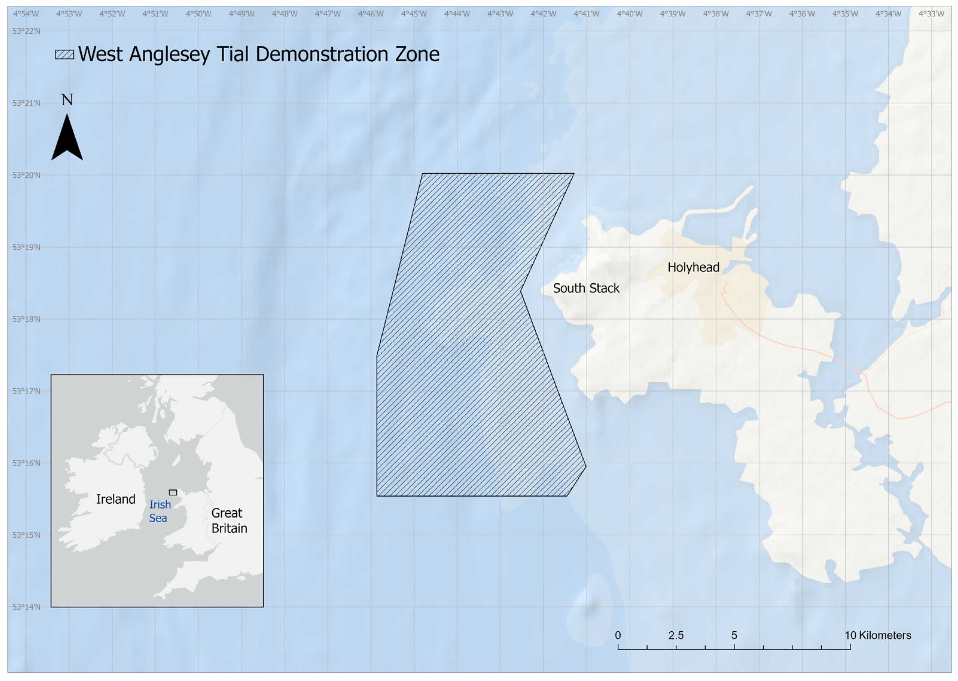
Tidal energy sites with gird connection at the European Marine Energy Centre (EMEC) at the Fall of Warness and at the Marine Energy Wales (MEW) West Anglesey Tidal Demonstration Zone, also known as Morlais, are facilitating the growth of commercialization (Figure 1). The MEW site comprises 35 km² of seabed around Holy Island in the Irish Sea off Wales. Support has been provided for the development of the site, for example, the EU ERDF funding of EUR 37.6 M aiming to boost commercialization [3]. The deployment of tidal energy converter (TEC) technologies within the zone is planned to scale up over time to a potential maximum electricity-generating capacity of 240 MW. This is the first large-scale third-sector community MRE project.

Despite the progress being made in several tidal stream energy projects as they approach commercialisation, there are still difficulties to overcome. For example, there is difficulty accessing tidal turbines underwater for O&M activities, which increases the associated costs [5]. In some tidal energy case studies, O&M accounts for 30% of the lifecycle cost of the project. The UK government has estimated that O&M accounts for 17% and 54% of the lifecycle cost for floating and fixed tidal energy devices, respectively [6]. In light of such high O&M costs, it is important to increase the reliability of tidal devices and reduce failure rates. Aside from O&M costs, it is also difficult to obtain a reliable and accurate prediction of the tidal turbine’s performance, and the associated wake generation, in such a complex deployment environment [7]. These uncertainties affect the costs and, thus, the LCoE of tidal energy projects.

Tools, modelling techniques and analyses have been developed to address most of these challenges. For example, reliability analyses such as the Failure Mode Effect Analysis (FMEA) have provided recommendations on improving turbine reliability by redesigning or monitoring conditions [8]. These recommendations to improve reliability will reduce unexpected failure rates. Many offshore O&M models and tools have been developed to decrease the uncertainty surrounding the O&M costs and provide recommendations on maintenance strategies. In [9] a comprehensive review of the existing tools up to 2020 is presented. Some of these O&M tools have been specifically developed for ocean energy (wave and tidal), and some are openly available such as the Wave Energy Scotland O&M tool for wave energy [10], DTOcean and DTOcean+ [11], and the SELKIE O&M tool for wave and tidal energy [12]. The MRE sector also employs computational fluid dynamics (CFD) tools to assist in device design and array configuration for maximising energy output [7].

Another key component of any MRE project is station keeping, not only because it keeps the device secured under extreme and often complex environmental loading, but also because it can influence power production, particularly for floating systems where the efficiency of the energy extraction depends on the motion of the device [13]. Station-keeping systems also represent a large portion of the total cost for a marine energy project: mooring and anchoring costs are often quoted as representing 10–30% of the installed cost for marine energy devices, as compared to 2–3% for floating oil and gas facilities [13]. This, coupled with the fact that arrays of devices will require efficient and reliable station-keeping systems to be produced in large numbers, makes the efficient design of station-keeping systems crucial to the success of marine energy projects. Many collaborative research and development projects, including GEOWAVE (2012–2015), SAFS (2017–2019), ELASTMOOR (2017–2020), CF2T (2018–2021), UMACK (2018–2021), and TIM (2019–2021), have focused on station-keeping systems. There are also several research and development projects considering the design of novel anchors, mooring systems, and floating platforms for offshore wind turbines, which represent a similar technical and economic challenge, including FLOTANT (2019–2022), PIVOTBUOY (2019–2022) and COREWIND (2019–2023).

Several techno-economic (TE) tools have been developed for renewable energy and have been reviewed in some detail by [14], a study which also outlined the expected merits of combining TE analysis with a Geographic Information System (GIS). This is due to the fact that many of the inputs involved in the TE analysis of renewable energy projects are inherently spatial in nature. These include the availability of the resource (for energy production), the distance to the closest adequate grid connection (for cable laying to point of export) and the distance to the nearest suitable port (for logistics as well as operation and maintenance). However, the application of a combined GIS-TE tool is new in the MRE sector.

This study integrates the application of four open-access tools developed for ocean energy as part of the SELKIE project [15] and investigates the techno-economic performance of hypothetical tidal stream energy projects in Wales. The four open-access tools are (i) generalised actuator disk computational fluid dynamics (GAD-CFD), a computation fluid dynamics (CFD) tool which analyses the configuration of the array and the turbine’s power curve using the time-series metocean data of the study location and the rotor diameters of tidal stream turbines considered; (ii) an F&M decision support tool which quickly and easily generates concept designs and cost estimates for the station-keeping systems; (iii) an O&M tool which analyses the operational expenditure (OPEX) and availability of a tidal project using the device’s failure rates and maintenance strategies over the project lifetime; (iv) an integrated GIS-TE tool which uses the outputs from the first three tools as inputs to the calculation of the net present value (NPV) and LCoE for each of the case studies. Generic 500 kW fixed and 2 MW floating HATTs are assumed for hypothetical farms of 2, 10, 40 and 100 MW capacity. This was to reflect projects of varying scales, ranging from the demonstrational to the commercial, and incorporating the two most common turbine variations used in tidal energy. The West Anglesey Tidal Demonstration Zone (Figure 1) is the study location for each.

The study has a two-fold contribution to MRE research. First, it demonstrates a practical application of integrating the four open-access tools (which can be used for both the tidal and wave energy sectors). Second, it demonstrates how to design a tidal energy project in an area with considerable potential for commercial scale project deployment and exhibits the computation of a project’s LCoE along with a thorough breakdown of the associated costs. This can assist the MRE community to employ these open access tools for real-world scenarios and analyse the techno-economic performance of future projects.

The rest of the article is structured as follows: Section 2 explains methods and data, results and discussion are presented in Section 3, and Section 4 provides the conclusion and recommended future work.

2. Materials and Methods

The techno-economic metrics of two hypothetical tidal projects at the Morlais site in Wales were assessed. The method’s framework is depicted in Figure 2. More information about the method’s features and descriptions of case studies are provided in this section.

The study used data representing bathymetry and metocean conditions for the site of interest. These are detailed in Section 2.1. The study also used some computed data and data from the literature, which are discussed further down and in this section.

The CFD model was used to obtain the power curves of fixed and floating HATT. The power curve was interpolated to hourly values of the flow at the study site to obtain the annual electrical power output from each tidal turbine. The CFD model was also used to examine the tidal farm configurations and provide an estimate of the farm’s wake losses. More information about the SELKIE CFD tool can be found on the SELKIE project website [16,17]. The key computational techniques used in the study are detailed in Section 2.3.

The specifications of F&M designs were obtained using the SELKIE F&M tools. These are a set of Python-based decision support modules built to facilitate concept design, cost estimation, and option studies for gravity-based foundations and anchors, suction caisson foundations and anchors, and catenary and taut mooring systems. Designed with emphases on simplicity and flexibility, these three tools can be used to provide initial size and cost estimates for these foundation anchors and mooring systems. Further information on the development of the Selkie station-keeping tools is available at [18,19]. The selection of the F&M system is explained in Section 2.4.

The lifecycle O&M costs of the tidal energy projects were examined using the SELKIE Logistics and O&M tool. The logics and computation process of the model are fully described in [20], and the application of the tool in case studies can be found in [21,22,23]. In summary, within the tool, normal distribution and Monte Carlo simulations are used to randomise failures per each scenario. The simulation begins when the user defines an input. The model will then generate an O&M task list based on the failure list for all maintenance activities to be performed. For each task, the model will include the following details: the component and equipment that needs to be maintained, the technicians and vessel(s) required, the base O&M assigned (fixed yearly operational cost), the percentage of power loss, the cost of spare parts and consumables, and the operation location (onshore/offshore). Using input data from the relevant ocean energy project, the model calculates the annual O&M expenditures and availability of the tidal/wave farm during the course of the project. Some of the input data include power curves, time-series of metocean data, port facility, characteristics and costs of vessels, components failure rates, repair data, technicians and spare-part costs. Section 2.5 explains the O&M model’s data and presumptions.

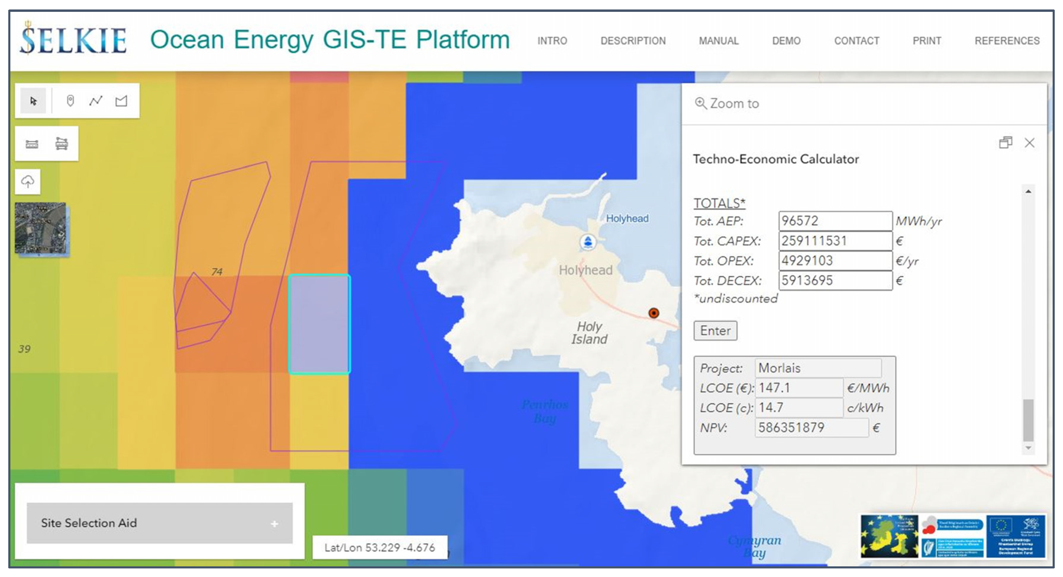
The Geographic Information System and Techno-Economic (GIS-TE) tool then calculates the anticipated LCoE and NPV for the hypothetical tidal energy projects using Equations (1) and (2) with inputs coming from the GIS, CFD, F&M designs as well as O&M modelling:

$$LCoE=\frac{{\sum }_{t=0}^{N_{farm}}\frac{{CAPEX}_t+{OPEX}_t+{DECEX}_t}{{(1+r)}^t}}{\sum _{t=0}^{N_{farm}}\frac{E_t}{{(1+r)}^t}},$$

(1)

where N_farm is the project lifetime, E_t is the energy produced by the farm in year t (MWh/year) and r is the discount rate for the project. NPV can be calculated as

$$NPV=-G_0+{\sum }_{t=1}^n\frac{{CF}_t}{{(1+r)}^t},$$

(2)

where CF_t is the cash flow (CF_t = R_t − X_t, where X_t is the expenses per year and R_t the revenues per year), t is the lifecycle years, G₀ is the initial investment and r is the discount rate.

The description of the GIS-TE tool can be found on the SELKIE website [24], and [14] provides a detailed explanation of the tool and much of the data contained within it. The methodology for employing the GIS-TE tool in this study, along with a description of some of the data that were more salient to the analysis, are provided in Section 2.1 of this article.

2.1. Site Data

With an existing site agreement for tidal energy deployment in place, this study was focused on the Morlais West Anglesey Tidal Demonstration Zone (Latitude 53.291° N, Longitude 4.743° W) comprising a 35 km² area of seabed just west of South Stack Lighthouse on Holy Island in northwest Wales (see Figure 1). The site has already facilitated the deployment of several TEC prototypes at varying scales and is regarded as having the potential to deliver up to 240 MW of electricity [25]. Data sourcing for current speed, wind speed, significant wave height, wave period, water depth, seabed, and proximity to potential port/grid opportunities for the location are briefly described here.

Current speed: The European North West Shelf Ocean Physics Analysis and Forecast product was used to model the tidal climate. This model is based on NEMO (Nucleus for European Modelling of the Ocean) and is forecast by both the UK Met Office North Atlantic Ocean forecast model and by the ECMWF Numerical Weather Prediction model. The model has a spatial resolution of 0.014° × 0.03°, or ~0.4–1.5 km, and an hourly temporal resolution. The variables used were the “Northward Current Velocity in the Water Column (vo)” and the “Eastward Current Velocity in the Water Column (uo)”. The time series applied was 1 January 2020 00:00:00 to 31 December 2020 23:00:00.

Wind speed: The ECMWF ERA5 dataset was chosen to model the wind climate. The product combines vast amounts of historical observations into global estimates using advanced modelling and data assimilation systems. It covers the entire globe, with a spatial resolution of ~30 km, and has an hourly temporal resolution. The variables downloaded were the “10 m U-component of wind (u10)” and the “10 m V-component of wind (v10)”. The time series applied was 1 January 2020 00:00:00 to 30 December 2019 23:00:00.

Wave height and period: The Atlantic–Iberian Biscay Irish–Ocean Wave Reanalysis product from the Copernicus Marine Service was used to model the wave climate. This model is based on MFWAM developed by Meteo-France. It is fed by the ERA 5 reanalysis wind data from ECMWF, covers the extents 19° W–5° W; 56° N–26° N, has a spatial resolution of 0.05° × 0.05°, or 3 to 5 km, and has an hourly temporal resolution. The variables used were “Spectral significant wave height (Hm0)”, “Spectral moments (−1,0) wave period (Tm-10)” and “Wave period at spectral peak/peak period (Tp)”. The time series applied was 1 January 2020 00:00:00 to 30 December 2019 23:00:00.

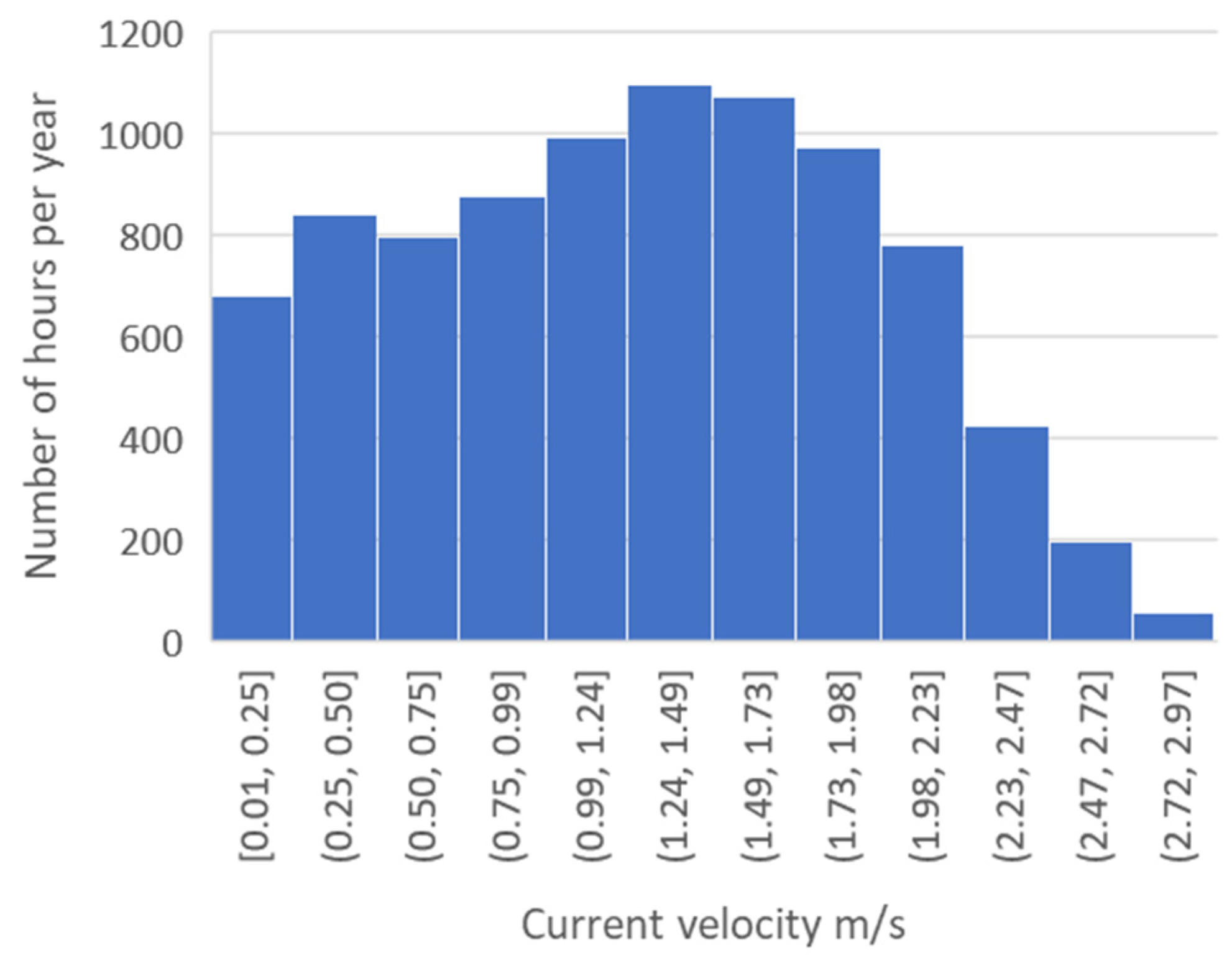
Figure 3 shows the histogram of the site’s current speed and

Table 1. Statistics of the site’s weather data and incident power density.

Variable	Average	Max	75th Percentile	25th Percentile
Current speed m/s	1.26	2.97	1.79	0.71
Incident power density (kW/m2)	1.93	13.38	2.95	0.18
Significant wave height (m)	2.60	13.21	3.35	1.5
Wind speed (m/s)	6.37	21.38	8.48	3.95

presents a few meteorological statistics for the research site based on the metocean data mentioned above. The location’s average current velocity is 1.26 m/s, and the mean incidence power density per square metre of flow is 1.93 kW/m².

Bathymetry and seabed character: The European Marine Observation and Data Network (EMODnet) provides open access data on both the bathymetry and seabed character for the European sea regions. The product used for representing water depth at the study site was the harmonised EMODnet digital terrain model (DTM). The latest release of this product has a spatial resolution of approx. 115 m. It is generated from bathymetric survey data sets, composite DTMs and satellite-derived bathymetry products, with any data gaps being filled through the integration of GEBCO Digital Bathymetry [26]. For seabed character, Folk-7 data are regarded as sufficient to inform the deployment of MRE infrastructure [27]. This classification system divides the seabed character into: Rock and Boulders; Coarse Sediment (Gravel ≥ 0% (or Gravel ≥ 5% and Sand ≥90%)); Mixed Sediment (Mud 95–10%; Sand < 90%; Gravel ≥ 5%); Mud (Mud ≥ 90%; Sand < 10%; Gravel < 5%); Sandy Mud (Mud 50–90%; Sand 10–50%; Gravel < 5%); Muddy Sand (Mud 10–50%; Sand 50–90%; Gravel < 5%) and Sand (Mud < 10%; Sand ≥ 90%; Gravel < 5%). The resolution of EMODnet Folk-7 data available for the study site was 1:250,000 [28].

Port and grid distance: The hypothetical deployment and O&M port chosen for this study was Holyhead. The port is regarded by Marine Energy Wales as a world-class deep-water port facility with the potential to support the MRE sector [29]. The distance of this port from the Morlais deployment site is approx. 8 km. The closest potential grid connection point to the site is Penrhos 132 kV Substation approx. 7 km from the deployment site, via the nearest possible beach landing opportunity at Trearddur Bay.

Accessibility: The accessibility of an offshore energy site is a critical factor in the cost of O&M because it will determine the availability of the farm to generate energy and, therefore, revenue. The limiting significant wave height and wind speed of a location have a major influence on the accessibility to the site, which varies by the selection of the vessel and the length of the weather window gap required for the offshore operation. For offshore wind, studies have calculated the accessibility of some sites [30]. Also, ref. [31] calculated an accessibility of 10–90% in the Scotwind sites for 15 floating offshore wind farms at different Hs limits and weather window gap lengths.

At the site of interest, using the time-series of wind and wave data described above, and depending on weather condition limits and minimum weather window gaps (e.g., 12 h and 24 h), the accessibility can vary significantly in different seasons, as illustrated in Figure 4. For a weather window gap of 12 h with Hs < 2.5 m and wind speed < 15 m/s, the Morlais site can achieve ≥80% accessibility for all seasons. However, for the tighter weather condition limits and a longer weather window gap, the accessibility will be much lower, especially in winter months. The O&M model used here considers the accessibility of the site when a component failure occurs based on the mean annual failure rate, weather window gap, mean time to retrieve the device, mean time to repair, port distance, and the type of vessels required to carry out the task. In this way, the availability of the farm for the study location was investigated.

2.2. Tidal Energy Converters

Two types of generic tidal stream energy turbines, which are the most common turbines developed by various turbine companies, wer considered in the study: Type (1), a HATT which is fixed to the seabed via a pile or gravity base, similar to concepts 1 and 2 in [8]; Type (2), a floating HATT which is moored to the seabed via mooring lines, similar to concept 3 in [8]. The rated power of the fixed turbine is 500 kW with a rotor diameter of 14 m and the power rating of the floating turbine is 2 MW with a rotor diameter of 22 m representing medium-to-large-scale turbines [6]. Examples of similar fixed tidal turbines are the Sabella D10 and SIMEC AR500 and of similar floating turbines are the Magallanes-ATIR and Orbital-O2.

From the techno-economic perspective, there are advantages and disadvantages for these two types of turbines when compared with each other. Fixed HATTs generally require expensive vessels equipped with cranes for installation and access, while floating turbines are usually more expensive to build, but require smaller vessels which reduces O&M costs [3]. The analyses of power curves, array configurations, mooring and foundation designs as well as data and parameters for the O&M and GIS-TE modelling of assumed tidal projects are explained in the following sections.

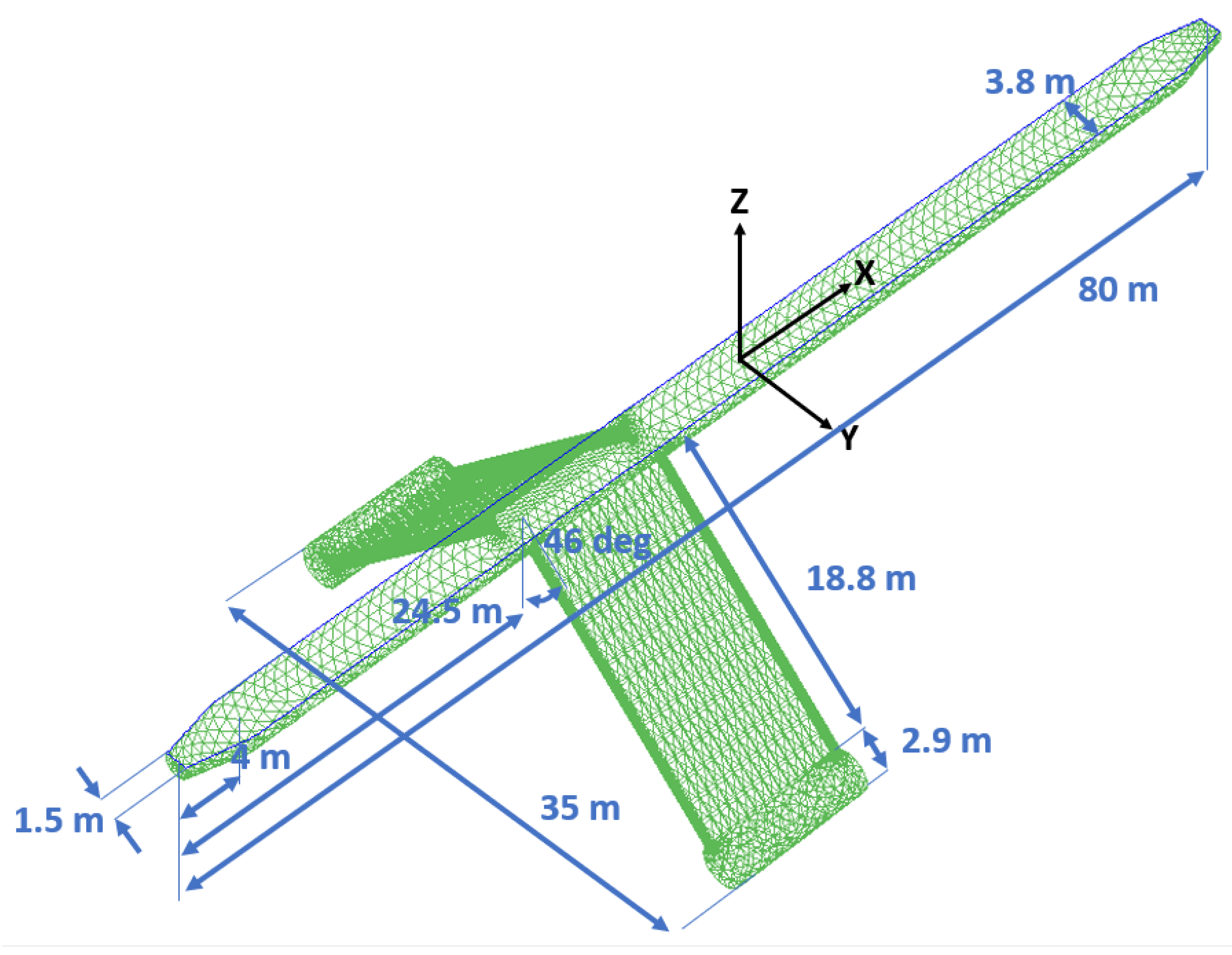
2.3. CFD Features

The CFD framework employed was based on the finite volume solver “simpleFOAM” of the OpenFOAM toolbox, which is a steady-state incompressible Reynolds-Averaged Navier–Stokes (RANS) solver. The turbulence was modelled with a k-ε RNG model, which has been demonstrated to show good accuracy for this class of problem [7,32]. From a modelling point of view, each turbine was represented as a blade box to reduce the mesh complexity of the simulation, while the nacelles of the turbines were ignored. The blade boxes, with diameters of 14 m and 22 m, were assumed to have a width of 0.1 D, which is 1.4 m and 2.2 m for the two rotors in question. The Generalised Actuator Disc (GAD) model, which is part of the OpenFOAM framework, was used for modelling the turbine. With this method, which is based on the classical Blade Element Method (BEM), the rotors are described as additional source terms within the Navier–Stokes equations [32]. The advantage of the method against the classic BEM is that it considers the losses along the foil through the computation of the distribution of downwash from the Prandtl Lifting Line theory, which considers the blade variable cross-section along the length, and it provides a dynamic variation in the Reynolds numbers [32]. With this rotor representation, a good accuracy is attained, while computational costs are kept to a minimum, which is crucial when simulating such large domains with the inclusion of a large number of rotors. Examples of the accuracy of the approach for single rotors and arrays of rotors can be found in [32] and [7], respectively. The framework also includes an active rotor control that establishes a maximum power for the rotors by a drop in rotational speed as the velocity upstream of the rotor increases, maintaining a constant tip speed ratio (TSR).

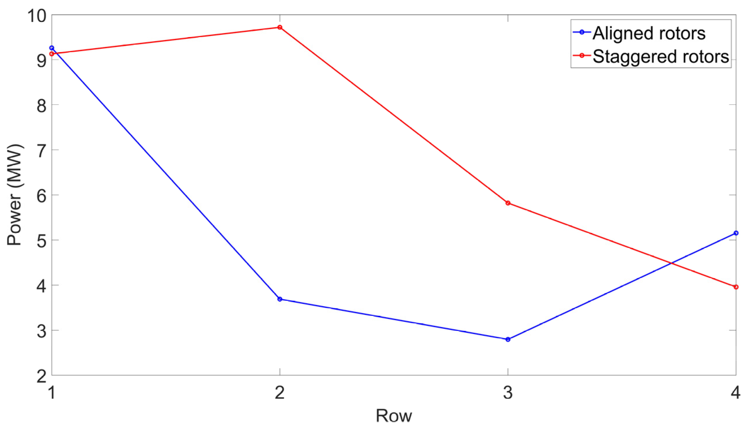
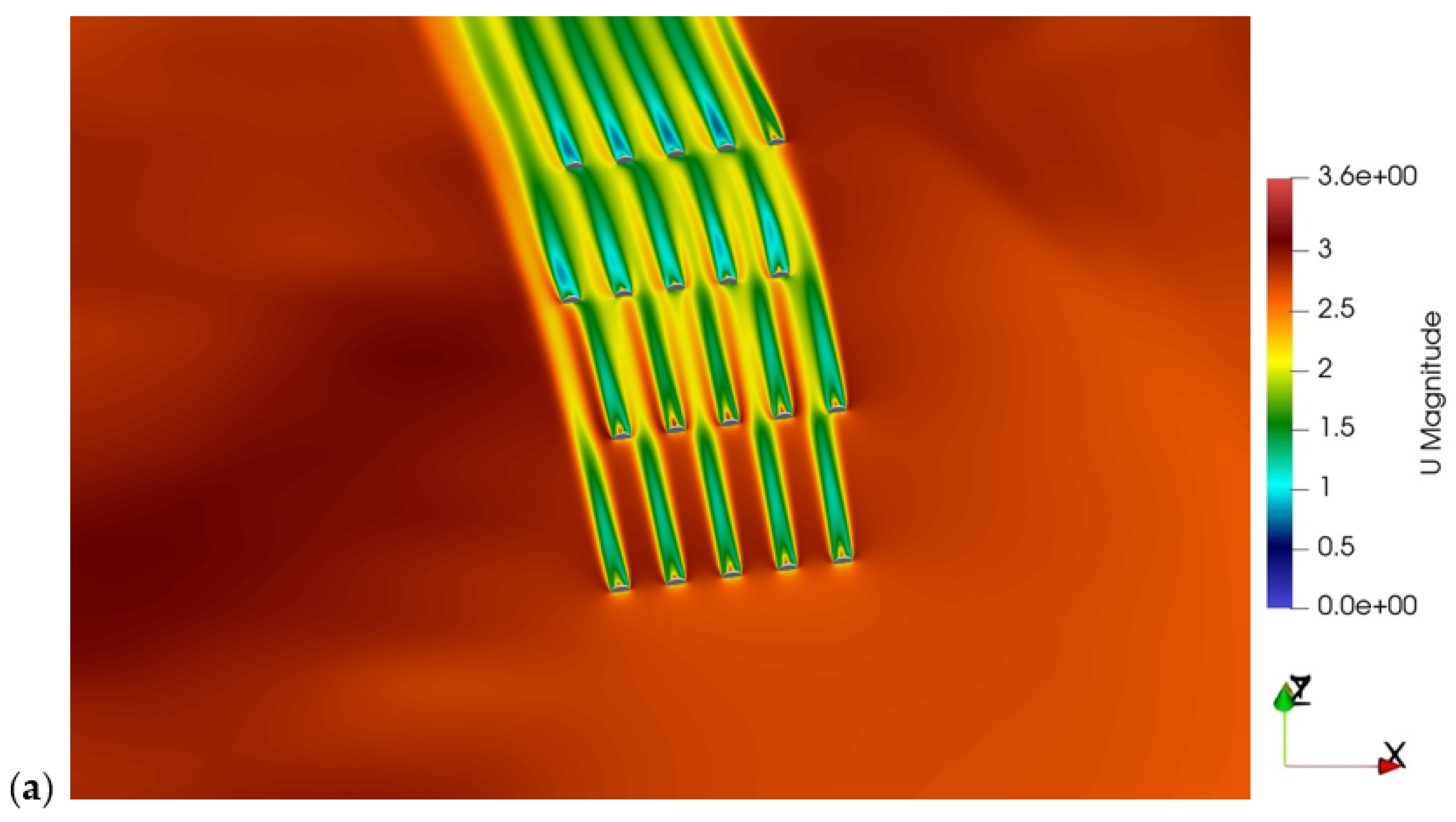
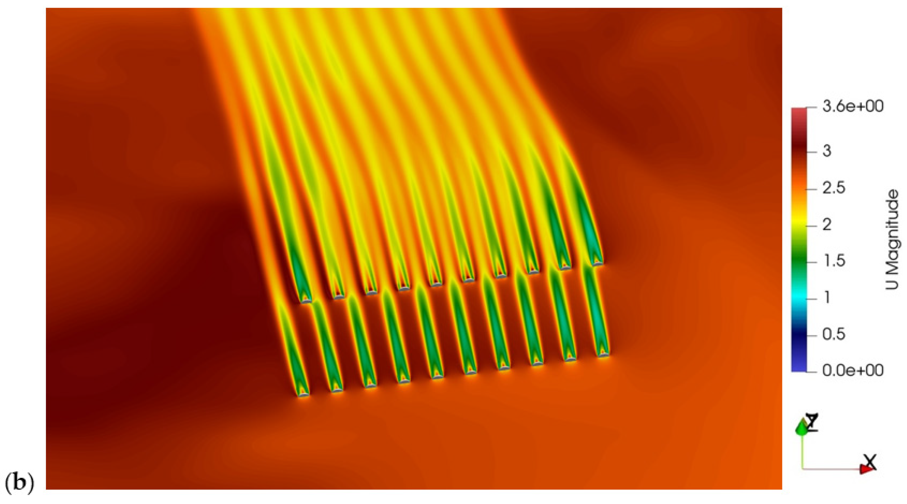
Using 20 floating and fixed turbine devices as an example, all simulated arrays have one of two configurations: rows of 10 rotors each, or rows of 5 rotors each. The arrangements investigated were the aligned and staggered configurations. Examples of the 5 rotor array configurations are shown in Figure 5. In the sections that follow, more information regarding the power curves of a single turbine and array designs are provided.

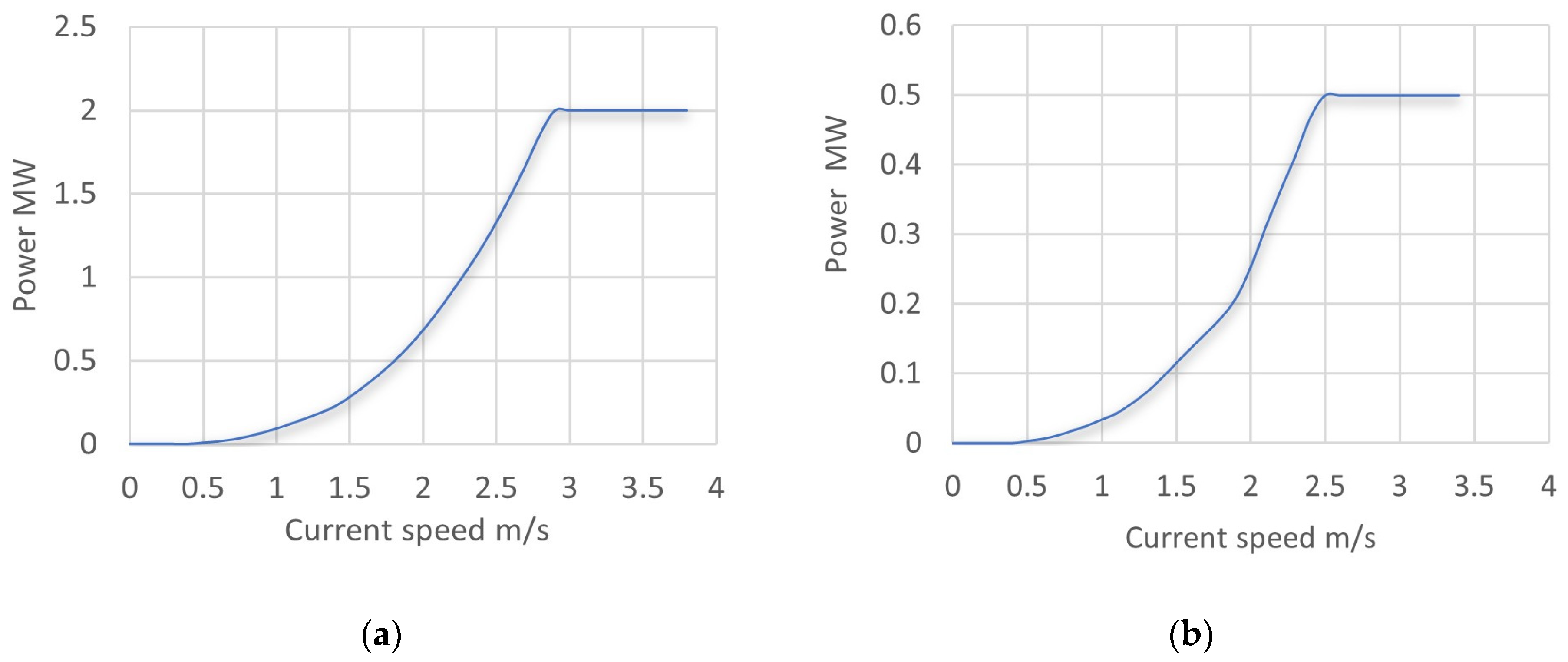
2.3.1. Power Output of a Single Turbine

The generic rotors used for the study were a scaled-up model of those used by the authors of [33] for their experimental studies. Two rotors were produced via dimensional scaling, as explained above: one based on the 500 kW device and one on the 2 MW device, with the diameters reported above. The chord and twist ratio distributions were kept as the experimental setup along the blade span. Moreover, the hydrofoils considered were the NACA63418 and NACA63422.

Several tests were conducted to obtain the power output of a single turbine while maintaining an optimal TSR of 3.67 and gradually increasing the input velocity. The inlet velocity was in the range between 0.5 and 5 m/s. The following equation is used to calculate the turbine’s power (P):

$$P=\frac{C_P\rho A{U}_{\infty }^3}{2},$$

(3)

where $\rho$ and $A$ are the water density and the cross-sectional area of the blade box, $C_P$ is the power coefficient calculated, and $U_{\infty }$ is the velocity at a distance of 2 diameters upstream of the rotor. The cut-off power of each rotor was set at 500 kW and 2 MW. After simulating all the inlet velocities within the range of interest, the power output was obtained by interpolating between the simulated values and the curve is presented in the Results section.

2.3.2. Array Configurations

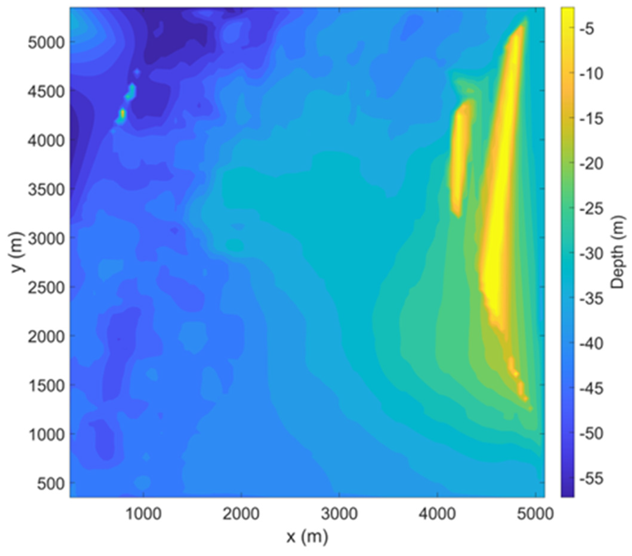
For analysing array configurations, a parallelepiped with dimensions of 2.5 km in width and 5 km in length (x and y directions, respectively) was chosen as the domain selection for the study location (Figure 5a). The cells of the mesh had an aspect ratio of 1 and the initial resolution was chosen to be 10 m (Δx = Δy = Δz = 10 m), with additional mesh refinement applied at the seabed and in the rotor and wake regions. A y+ value of 300 was employed here. The mesh used in this study consisted of 27.1 million elements; the majority of these were hexahedral elements, with the remainder being prisms. The World Geodetic System 1984 (WGS84) was used to convert the location bathymetry data from the Global Positioning System (GPS) longitude–latitude format into Cartesian coordinates. The bathymetry of the domain employed can be found in Figure A1 of Appendix A. Moreover, real-time current velocity data described in the previous section were used as the velocity inlet of the computational domain. In the simulations, two cases of velocities were used, the maximum and the most frequent. The maximum velocity was employed to acquire the optimal set up of the configuration, while the most frequent one was employed to obtain more indicative results in terms of power production prediction. When the velocity measurements were analysed, it was found that the directional components for the target velocities were consistent with a fixed aspect ratio. Thus, their ratio was determined to be $\frac{U_y}{U_x}\cong 0.16$. This ratio was used throughout the study to define the inlet velocities. The maximum current velocity was $U_{\mathrm{\infty }}=2.83\mathrm{m}$/s, while the most frequent one $U_{\mathrm{\infty }}=1.63\mathrm{m}$/s, and their corresponding components were calculated according to the ratio $\frac{U_y}{U_x}$. The Reynolds number for this problem is $2.3\times {10}^7$ and $3.5\times {10}^7$ for the 14 m and 22 m diameter rotors, respectively.

The domain’s east and south boundaries served as velocity inlets for the boundary conditions, while the west and north served as outlets. At these boundaries, the velocity was assumed to follow the 1/7th power law profile along the depth, which is a realistic assumption for the study site according to [34]. Since the velocity was measured at a single point, as acquired from the model explained in the previous section, the measurement value was employed throughout the entire plane of the inlets. In this way, the rotors were set at a distance from the boundaries, and the flow was given enough space to fully develop at the rotors. Because the domain was a section of the ocean, the velocity at the outlet had zero gradient normal to the plane and its pressure was set to 0 at that plane. The slip condition, which depicts open-water circumstances, was applied to the top plane, which represented sea level, while a no-slip condition was applied to the bottom plane, which represented the seabed. The wall roughness height was set to (Ks) 0.01 and the roughness constant (Cs) was set to 0.5. Finally, for the turbulence model, an intensity of 1% and a dissipation of $9.7\times {10}^{-6}$ were set.

The model was solved in OpenFOAM using the SIMPLE velocity–pressure coupling algorithm. The convergence criteria for velocity, pressure, and turbulence variables were defined to be $1\times {10}^{-4}$, $2\times {10}^{-4}$ and $1\times {10}^{-3}$, respectively.

The arrays were placed at the centre of the domain arbitrarily. In the floating case, the tips of the rotors were located at 2.5 m below the sea surface, while in the fixed-bed case, they were placed at 2/3 R above the seabed. In all array cases, the rows were spaced 10D apart, and on each row, the rotors were 3D away from each other (Figure 5). These spaces have proven to be the optimal scenario, preventing downstream turbines operating in wakes when a staggered configuration is used, where the position of rotors in a downstream row is midway between the lateral upstream row rotor position [32,35]. However, for the aligned configuration, the lateral position of the downstream rotors is immediately behind the upstream rotors and, hence, these are more likely to be placed within the upstream wakes.

2.4. Foundations and Mooring

Modelling the F&M system designs of the two HATTs of the study required information on not only the type of device but also the local metocean data (bathymetry, wave, and current climates) and seabed conditions (the type and load-bearing characteristics of the soil).

In this scenario, the 500 kW bottom-fixed tidal turbine was secured to the seabed via a gravity-based foundation. The Selkie gravity-based foundation and anchor tool was used to design a simple rectangular concrete foundation to secure the turbine to the seabed. Here, the gravity-based foundation was developed both with and without a perimeter skirt, which can provide greater lateral resistance, and the total volume of foundation material required (concrete in this instance) was determined in each case.

The primary inputs for the design of the foundation were the local seabed and metocean conditions, which were obtained from the Selkie GIS-TE tool, together with some standard assumptions relating to the soil properties obtained from consultations with experts in the field, as shown in

Table 2. Key input data used in the design of the fixed turbine’s foundation.

Design Parameter	Value
Hub height (m)	18.3
Rotor diameter (m)	14
Mass (t)	150
Average water depth across the array (m)	32.8
Significant wave height with 50-year return period (m)	7
Corresponding average wave period (s)	9.38
Corresponding peak wave period (s)	10.42
Peak current velocity (m/s)	2.774
Seabed slope (degrees)	0
Soil type	Granular (very dense sand)
Coefficient of friction (soil-soil)	0.78
Coefficient of friction (concrete-soil)	0.65
Saturated unit weight of soil (kN/m3)	20
Friction angle (degrees)	38
Cohesion (kPa)	0 (granular soil)
Foundation thickness (m)	1.5 (user specified)
Depth of perimeter skirt (m)	0.5 (user specified)
Safety factor for soil parameters	1.15
Safety factor for design checks	1.3
Maximum horizontal load for bottom-fixed turbine (kN)	359.3
Maximum vertical load for bottom-fixed turbine (kN)	1500
Maximum overturning moment for bottom-fixed turbine (kNm)	6575

. It should also be noted that for the fixed turbine, the diffracted wave forces were assumed to be minor compared to the thrust force and so were neglected from the calculation.

The 2 MW floating turbine was secured using a catenary mooring system connected to gravity-based anchors. For the catenary mooring system, the open-access boundary element code NEMOH (v3.0.0) [36] was used to calculate the exciting forces on the floating turbine in 6 degrees of freedom between the frequencies of 0.016 and 0.32 Hz. The added mass and damping coefficients were also computed. The added mass, radiation damping, and excitation forces for the surge, heave, and pitch motions were then used to generate response amplitude operators (RAOs) for the design of the mooring system. The mooring design was then carried out using the Selkie F&M tool [18]. The key design constraints were the horizontal offset limit of 25 m and the vertical anchor load limit of 0 kN (as is typical for a catenary mooring system).

To secure each mooring line, the Selkie gravity-based foundation and anchor tool [18] was again used to design a rectangular concrete anchor. The results will again be presented for the anchor with and without a perimeter skirt. The local seabed conditions and design assumptions were again taken from Table 2, but in this case, the anchor was not subject to vertical load or an overturning moment; the maximum horizontal load was calculated as 1227.9 kN. As above, the Selkie gravity-based foundation and anchor tool was used to identify the minimum dimensions of an anchor which passes the necessary design checks for bearing capacity, sliding, and overturning.

2.5. Reliability and Cost Data

Reliability information for tidal projects is scarce in the literature since there have not been many tidal stream device deployments and because intellectual property is so sensitive. For an assumed 25-year project life, the failure rate of tidal turbines in a high-level generic subsystem, such as that shown in

Table 3. Failure rates and repair data for O&M model.

Turbine, Electrical, and Substructure	Failure/Year *	MTTR	Onshore–Offshore		Spare Part (EUR/Device/Failure)
			Fixed	Floating	Fixed	Floating
Blade—minor	0.105	7	Onshore	Offshore	1000	1300
Pitch—minor	0.383	9	Onshore	Offshore	1900	2500
Gearbox—major	0.077	30	Onshore	Onshore	80,000	100,000
Gearbox—minor	0.052	5	Onshore	Offshore	3500	4500
Generator—major	0.015	40	Onshore	Onshore	50,000	62,500
Generator—minor	0.256	7	Onshore	Offshore	4500	5850
Cables—minor	0.167	8	Offshore	Offshore	1500	2000
Electrical, grid and misc. minor	0.140	8	Onshore	Offshore	2500	3250
Fixed substructure minor	0.087	5	Onshore	Offshore	2000	-
Floating structure minor	0.981	12	-	Offshore	-	10,000
Mooring lines—minor	0.149	6	-	Offshore	-	3000
Anchors—minor	0.158	10	-	Offshore	-	6000
Sum	1.3 (Fixed T)	119			9851	23,457
	2.5 (Floating T)	147

* The mean annual failure rates are for an indicative generic commercial tidal turbine with assumed built-in redundancies and the planned maintenance as explained in the text.

, was obtained from the available data for offshore wind turbines [37,38,39] with some considerations which reduce unexpected failures, particularly major failures, for a future commercial tidal turbine. These include the building redundancy of some critical components such as sensors, control systems, pumps and brakes, which contribute greatly to the total number of unexpected failures over the lifetime of a project [37], and adapting an annual scheduled planned maintenance (PM) strategy for summer months [40]. While redundancy will increase CAPEX, the costs of scheduled maintenance activities are considered in the O&M model. A value of 0.068 is allocated to major gearbox and generator failures [6].

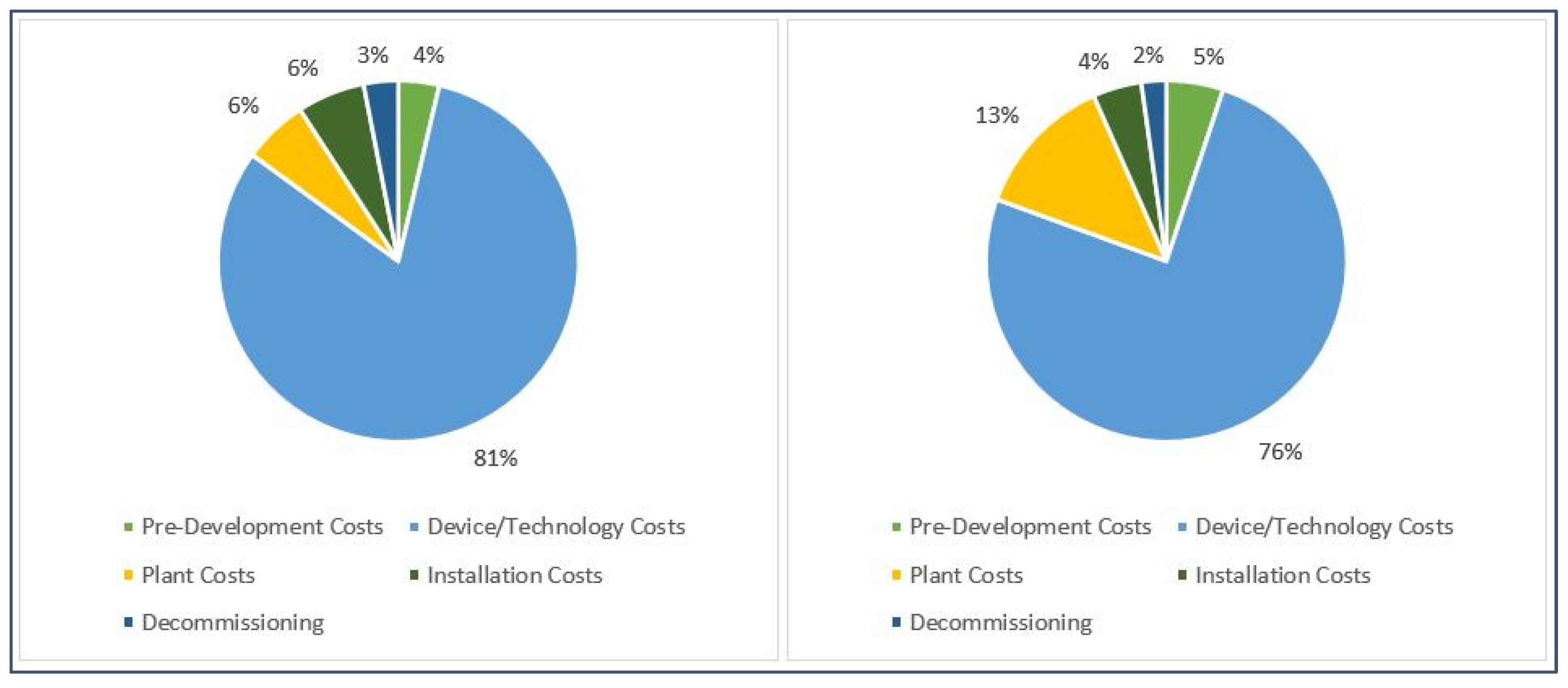
The annual PM activities include, for example, routine inspection, cleaning, the replacement of hydraulic fluids and filters, and other repairs and replacements [37]. The spare-part cost for a PM is assumed to be, on average, around 0.5% of the total structural device cost. An indicative cost breakdown per MW capacity of generic tidal stream devices by [41] shows that the cost of the device would account for around 41% of the CAPEX. In the MyGen project, the typical CAPEX/MW for a 10 MW tidal stream array is around 3.0–4.4 million EUR/MW [42]. From this rough estimate, it is assumed that the prices of the commercial fixed and floating devices are circa EUR 1.5 million and EUR 4 million, respectively. These costs include all aspects associated with the tidal turbine including all parts and assembly. Therefore, the spare-part costs for PM of a fixed turbine and a floating turbine are EUR 7500 and EUR 20,000, respectively. The fixed turbine’s PM is performed every two years and takes three days (72 h) per turbine, while the floating turbine’s PM occurs annually and lasts four days (96 h). Each turbine’s PM needs 5 technicians, and the PM tasks of both fixed and floating turbines are carried out onshore.

Three types of vessels are considered for the O&M model: (i) A multipurpose vessel for performing on-site minor repairs on floating turbines. The vessel has an average speed of 20 knots, a fuel consumption of 280 litres per hour and a daily rental cost of EUR 10,000. The maximum Hs and wind speed operation limits for this vessel are assumed to be 1.5 m and 15 m/s, respectively. These assumptions are based on expert consultation. (ii) A small tug vessel for major repairs of floating turbines to tow the devices back to shore. This vessel operates in a maximum of 1 m Hs and 12 m/s wind speed with a daily rental cost of EUR 4500 (its average speed and fuel consumption are 10 knots and 450 L/h, respectively [43]). (iii) A small dynamic positioning (DP) multipurpose vessel equipped with a crane for all minor and major repair tasks of the fixed tidal turbines. The daily rent, mobilisation cost and mobilisation time of the DP vessel are assumed at EUR 25,000, EUR 50,000 and 48 h, respectively. The average vessel speed is 12 knots and it can operate at a maximum Hs of 2.5 m and wind speed of 20 m/s [44].

The mean time to repair (MTTR) of 5 to 40 h, technician numbers of 2 to 5, and spare-part cost of EUR 1000 minimum for a minor repair up to a maximum of EUR 100,000 for a major repair (e.g., generator replacement) are obtained mainly from the available data for offshore wind turbines [45,46] (Table 3). The spare-part costs are slightly adjusted for TECs, which are considerably smaller than offshore wind turbines [37,39].

The CAPEX inputs for the TE analysis came from both the literature and the outputs of the O&M model as well as the F&M design modelling performed for this study. Development and consenting costs are those associated with environmental surveys, metocean assessments, geological surveys, etc. The associated value for this was obtained from a study for offshore wind. Costs associated with foundations and mooring were derived by taking the volume of concrete and length of mooring (0 m for fixed) proposed for the project through the F&M modelling, as described in Section 2.4. The total volume of the foundation with a perimeter skirt was applied to a standard cost per volume of concrete (see

Table 4. CAPEX inputs.

Attribute	Value	Source
Development and consent (EUR/MW)	135,000	[47]
Unit price of a fixed turbine (EUR/TEC)	1,500,000	See Section 2.5
Unit price of a floating turbine (EUR/TEC)	4,000,000	See Section 2.5
Mooring chain (EUR/m)	250	[48]
Concrete (EUR/m3) *	380	[49]
110 kV export cabling cost (EUR/km)	427,000	[50]
Export cabling length (km)	9	Site-specific
20 kV intra-array cabling cost (EUR/km)	87,000	[50]
Intra-array cabling cost	N/A	Array specific
Onshore grid connections (EUR/MW)	42,000	[50]
Diving work (EUR/day)	3500	[50]
Export cabling installation cost (EUR/km)	282,000	[50]
Array cabling installation cost (EUR/km)	123,000	[50]
Offshore logistics (EUR/MW)	4300	[47]
Decommissioning (% of installation)	50	[47]

* The foundation of a fixed turbine and the four gravity-based concrete anchors of a floating turbine are predicted to cost 77,720 EUR/MW and 190,882 EUR/MW, respectively (see Section 2.4).

). All other CAPEX cost inputs were obtained from the literature. A list of all CAPEX inputs can be found below in Table 4. As there is much uncertainty regarding decommissioning expenditure (DECEX) for tidal energy projects, this was taken as 50% of the installation costs, in accordance with figures given for offshore wind [47] (Table 4).

3. Results and Discussion

In this section, the key findings are presented, including the power curves of the two tidal turbines that were the focus of the study, array configurations, and F&M system designs, as well as the O&M outcomes and techno-economic results for the various project scales.

3.1. Power Curves and Array Configurations

The power curves of fixed and floating tidal turbines that were obtained using the approach given in Section 2.3.1 are shown in Figure 6, and their respective power outputs are reported in Section 3.3.

The outcomes of comparing the aligned and staggered array layouts are shown in Figure 7 and Figure 8. Figure 7 compares the power outputs for these formations using examples of five rotors in four rows of floating turbines. The results in Figure 7 show that the total power output of the staggered configuration was about 37% higher than the aligned configurations. In the staggered formation, there was a marked increase in power output from the second row of rotors. This is due to the increase in bypass flow velocity that occurs between laterally spaced rotors [34]. The staggered formation was designed to ensure that the rotors in the second row were not positioned within the wake of the front row, and so they benefitted from this increased bypass flow velocity. Further downstream, the performance of the rotors dropped as these were now influenced by the slower flows due to the wakes from the upstream rotors. The performance in the aligned array shows a significant drop in performance for the second and third rows due to the rotors being placed fully within the wake of the upstream rotors. However, there was an increase in performance in the fourth row, which appears to be due to the influence of the bathymetry on the flow characteristics at this location (Figure 7).

Figure 8 compares the staggered configuration of four and two rows for the example of 20 floating rotors. The two configurations consisted of one with two rows of ten rotors each, and another with four rows of five rotors each. The figure presents the velocity fields produced for the rows of 5 rotors (top) and 10 rotors (bottom). It is apparent that a configuration consisting of two rows would generate more power due to the reduced wake interactions between rows. Although such rotor fences appear to be the best practice, topological constraints sometimes render them ineffective, particularly for a large number of turbines. Nevertheless, based on the configuration results from the CFD modelling, the study assumed negligible wake losses for 10 rotors in two rows and average wake losses of 5% for the bigger projects.

3.2. Foundation and Mooring Types and Dimensions

Based on the design assumptions and procedures outlined in Section 2.4, the following dimensions were obtained for the gravity-based foundation used to secure the bottom-fixed tidal turbine: the foundation without a perimeter skirt was 5 m long, 14.25 m wide, and 1.5 m high, with a total volume of 106.88 m³, whereas the foundation with a perimeter skirt was 5 m long, 13.5 m wide, and 1.5 m high, with a total volume of 101.25 m³. The results show that the perimeter skirt provided greater horizontal resistance, which enables savings in both the weight and volume of foundation material required.

The floating turbine’s main dimensions are listed below, and Figure 9 displays the numerical mesh used in the NEMOH simulations: the hull tube was 80 m long, 3.8 m in diameter, and extended to a height of 1.5 m above the surface. Its displacement was 600 m³ and its maximum depth below the surface was 2.3 m.

Figure 10 depicts the final design of the mooring system: a four-leg configuration with two fore and two aft lines, with an anchor radius of 360 m, line length of 335 m, chain diameter of 114 mm, total offset at 13.79 m (mean offset was 12.04 m and dynamic offset was 1.75 m), and a maximum horizontal load on each anchor of 3678 kN. For the techno-economic modelling, the chain diameter and length were the key outputs. A standard cost per unit length for a given diameter (Table 4) can be used to calculate the resulting CAPEX for the mooring chains.

The following dimensions were obtained for the gravity-based anchors used to secure each mooring line: without the perimeter skirt, the anchor was 14.24 m long, 14.75 m wide, and had a total volume of 315.28 m³. With the perimeter skirt, the anchor was 11.75 m long, 14.25 m wide, and had a total volume of 251.16 m³. As with the gravity-based foundation, the perimeter skirt provided more horizontal resistance, which enabled reductions in both the weight and volume of anchor material required. A standard cost per volume of concrete (Table 4) can again be used to calculate the CAPEX for the anchor foundation (see Table 4).

3.3. O&M Costs

For the purpose of the techno-economic analysis of the projected tidal arrays, the 25-year lifecycle O&M costs of 2, 10, 40, and 100 MW fixed tidal projects and floating tidal projects were obtained for 10 simulations. A summary of the mean annual O&M costs is presented in

Table 5. Mean annual OPEX of tidal projects.

Farm Capacity (MW)	Fixed Tidal OPEX				Floating Tidal OPEX
	EUR/year	EUR/kW	EUR/MWh	% Share of Fixed OPEX	EUR/year	EUR/kW	EUR/MWh	% Share of Fixed OPEX
2	652,843	326	253	35	344,590	172	191	75
10	2,244,921	224	175	21	884,450	88	98	53
40	7,215,482	180	142	12	2,238,842	56	62	27
100	13,894,979	139	111	11	4,949,103	49	55	15

. The percentage breakdown of OPEX for the 100 MW project examples is shown in Figure A2 of Appendix A, which indicates what costs are most influential for OPEX. The mean annual energy production of a 500 kW fixed tidal device and a 2 MW floating tidal device is around 702.7 MWh and 2024.3 MWh, respectively (per turbine). The average availability for fixed tidal projects and floating tidal projects is 97.3% and 95.5%, respectively.

The effects of economies of scale on the decline in OPEX, in terms of EUR/kW, for each technology can be approximated based on the results of Table 5. This demonstrates that the O&M expenses for fixed tidal projects may be lowered by 14%, and for floating tidal projects by 20%, by doubling the farm’s capacity for each project. The following section’s LCoE analysis uses the O&M tool outputs for each hypothetical project, including the mean annual OPEX, mean annual MWh energy production, and availability factor. The next section also looks at how economies of scale affect the projects’ LCoE.

The results from Table 5 indicate that fixed tidal projects have an OPEX that is much higher than floating tidal projects. This is owing to the highly expensive DP craned vessels (hiring and mobilisation, Section 2.5) required for fixed turbines and their longer retrieval time. For example, it can be seen in Table 5 that the annual OPEX for a 100 MW fixed tidal project at the study site would cost 64% more in terms of EUR/kW and 50% more in terms of EUR/kWh than the equivalent-scale floating tidal project. The lower percentage reduction in EUR/kWh may refer to the higher capacity factor (by 33%) and higher availability (by 1.8%) of fixed tidal energy projects compared to floating projects. The capacity factor, which, in this case, is 16% for the fixed turbine and 12% for the floating turbine, is still low when compared to what is projected for a commercial tidal turbine, which is forecast to be at or above 35% [3,51]. The study’s power computation, according to Section 2.3, was based on broad descriptions of tidal devices found in the literature. This can be improved when valid data from experimental studies are incorporated into the model.

Based on the OPEX estimated by Ocean Energy Systems (OES) [51], the minimum and maximum OPEX of commercial tidal energy projects are 23.2 EUR/kWh and 102.9 EUR/kWh, respectively. As shown in Table 5, the OPEX is high for both the fixed and floating turbine projects. This is notably true for the fixed-turbine projects and perhaps indicates that scenario analyses should be adopted to optimise OPEX strategies. Although OPEX optimisation and sensitivity analyses fall outside the scope of this study, a prior study [23] looked at alternative cases that might be optimised, such as reduced mean time to failure, mean time to repair (including transit time to and from the port), and logistics options utilising the same O&M tool in this study.

3.4. Techno-Economic Analysis

On the GIS interface, an area within the West Anglesey Tidal Demonstration Zone was clicked in order to activate the TE Calculator at this site. After selecting a discount rate of 7.5%, the energy production and breakdown of CAPEX, OPEX, and DECEX were then entered (which are summarised in Figure A3 of Appendix A (for the example of a 100 MW floating tidal project)), before running the TE Calculator to reveal the LCoE and NPV of the hypothetical projects. The results of running all eight simulations (for fixed and floating turbines) are shown in

Table 6. Techno-economic analysis summary and results.

Farm Capacity (MW)	Fixed Tidal Project
	Energy (MWh)	CAPEX (EUR)	OPEX (EUR)	DECEX (EUR)	NPV (EUR)	LCoE (EUR/MWh)
2	67,550	13,337,668	7,170,152	1,493,218	−4,762,689	461
10	341,125	40,971,342	24,655,892	2,167,955	52,022,634	237
40	1,367,050	145,988,869	79,247,399	5,113,805	271,613,707	191
100	3,418,900	357,388,923	152,388,433	11,413,251	742,578,512	173
Farm Capacity (MW)	Floating Tidal Project
	Energy (MWh)	CAPEX (EUR)	OPEX (EUR)	DECEX (EUR)	NPV (EUR)	LCoE (EUR/MWh)
2	45,925	11,428,821	3,784,620	1,400,164	−7,241,531	548
10	239,250	31,427,103	9,713,884	1,702,685	40,080,276	222
40	964,275	106,971,912	24,589,127	3,001,805	223,198,379	159
100	2,414,300	259,111,531	54,136,174	5,913,695	586,351,879	147

. The percentage breakdown of CAPEX for the example of the 100 MW projects is shown in Figure A4 of Appendix A.

It is evident from Table 6 that, due to economies of scale, the NPV increases and LCoE decreases as the farm sizes increase. It is estimated that any project less than 10 MW in capacity will not break even as the NPV is negative. Compared to fixed arrays, floating turbine projects have better prospects for both CAPEX and OPEX; however, as discussed in Section 3.3, OPEX has a more noticeable impact. As it is taken as a percentage of the installation cost, DECEX is also highest for the fixed projects. In terms of energy production, it is expected that a farm with a greater number of lower-capacity (500 kW) fixed devices will produce more energy per year than that with a smaller number of higher-capacity (2000 kw) floating devices for a project of the same scale (MW). This is likely a result of the fixed turbine in the study having a higher capacity factor, as previously noted. The percentage breakdown of the lifecycle costs for the example of the 100 MW projects are shown in Figure A5 of Appendix A.

Overall, the key performance indicators (KPIs) reveal that a floating tidal energy farm will generally be more economically feasible than fixed farms of the same capacity at the site of interest. However, the lowest values of 147 EUR/MWh, for the 100 MW floating farm, are still quite high in comparison to that of fixed offshore wind, which has been estimated to have an LCoE of as low as 58.43 EUR/MWh for fixed installations [52]. To compare with floating offshore wind, a study estimated values to range from 82 to 236.7 EUR/MWh [48]. Previous studies on the LCoE of tidal energy have produced values of as low as 95 EUR/MWh, converted from GBP [53], but as high as 260 EUR/MWh [54]. Meanwhile, the Strategic Energy Technology (SET) plan for ocean energy set a target of 100 EUR/MWh for tidal energy by 2030 [55], the same start year as that chosen for this study.

The analysed LCoE in Table 6 reveals economies-of-scale factors of ~16% and ~21%, respectively, for fixed and floating tidal projects, respectively. On this premise, and assuming the SET LCoE target of 100 EUR/MWh, fixed and floating tidal projects with a minimum capacity of around 800 MW and 400 MW, respectively, may well achieve this target.

4. Conclusions

The feasibility of tidal energy project development was assessed at a prospective site with an existing grid connection in Wales, with an emphasis on the configurations, F&M designs, O&M, and LCoE metrics. Two generic categories of tidal energy technology, 500 kW fixed and 2 MW floating, were considered in hypothetical 2 MW, 10 MW, 40 MW, and 100 MW projects. Four open-access tools were used in the study to model the associated array configuration (CFD), F&M design, O&M, and techno-economics. To illustrate the applicability of each of the employed tools, the study used site-specific data, including bathymetry, time-series metocean data (current velocity, wind speed, and significant wave height), seabed conditions (the type and load-bearing characteristics of the soil), cost data from the literature, and educational assumptions.

The results of the CFD modelling demonstrate that the configuration of the array, together with the influence of the bathymetry on the turbine wakes, can significantly affect the power generation from the array, particularly with respect to the downstream turbines. The CFD tool will enable developers to use site-specific bathymetry and flow characteristics to fine-tune the spacing between individual turbines, leading to the design of arrays with optimum power output for a particular deployment location. Whilst the optimum array configuration at one location is unlikely to be the optimum array configuration at all locations, the advantage of the CFD tool is that it allows the user to look at the flow profile and then adjust the position of individual turbines to improve the performance of the array as a whole.

For the F&M modelling results, the foundation with a perimeter skirt was selected as the variant for the subsequent techno-economic calculations due to its high resilience and cost-effectiveness in terms of weight and volume of foundation materials. The model estimated the volume of the gravity-based foundation for a fixed turbine to be roughly 101 m³, the combined volume of the gravity-based anchors for a floating turbine to be 1005 m³, and the total length of the mooring lines to be 335 m with a chain diameter of 114 mm. These results give a good indication of the volume of materials likely to be required for future tidal energy deployments, yet the values will vary from one site to another, thus requiring further scenario analyses using the F&M tool if accurate site-specific results are desired. Furthermore, the integration of a hydrodynamic and mooring analysis into the LCoE calculation improved the output of the latter, thus allowing greater certainty in the results.

In terms of the O&M modelling, for the corrective maintenance activities, it was expected that a fixed turbine and floating turbine would experience 1.3 and 2.5 respective failures annually, with mean annual spare-part costs per device of EUR 9851 and EUR 23,457. The spare component costs, as a percentage of the tidal turbine pricing, for the annual and bi-annual PM of the floating and fixed turbines were EUR 20,000 and EUR 7500, respectively. The mean annual OPEX for project scales of 2 MW to 100 MW ranged between 253 EUR/MWh and 111 EUR/MWh for the fixed turbine, while they were in the range of 191 EUR/MWh to 55 EUR/MWh for the floating turbine. The results showed that, with the implementation of appropriate planned maintenance, availabilities of 97.3% and 95.5% for fixed and floating tidal projects, respectively, can be achieved.

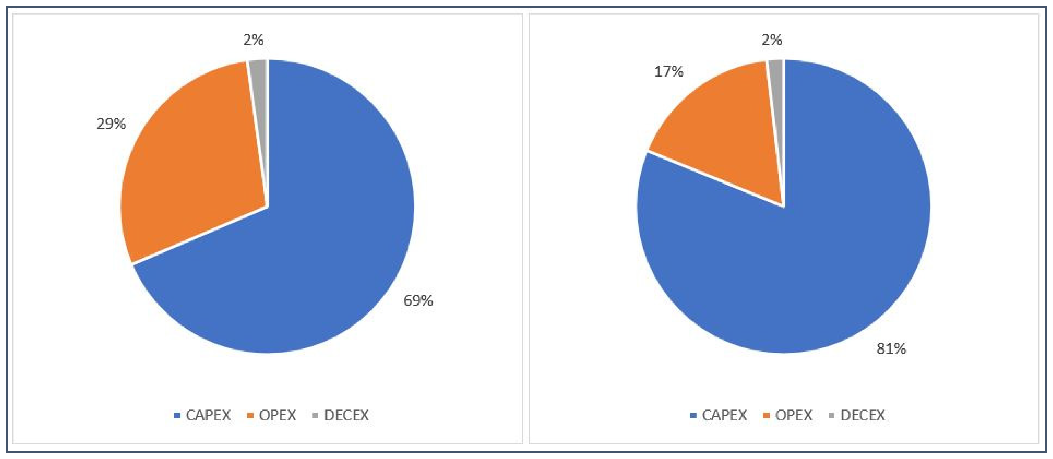
The outputs of the GIS-TE tool indicated that projects involving floating turbines would typically be more economically viable than those with fixed turbines of the same capacity. This was likely a result of fixed tidal projects having significantly higher CAPEX and OPEX compared to floating projects, even though fixed projects were also found to produce more energy than floating farms of the same capacity. At the site of interest, the 100 MW floating project was found to produce the lowest LCoE of 147 EUR/MWh. Yet, when compared, for instance, to the SET objective of 100 EUR/MWh for tidal energy by 2030, this figure is still considerably off target. However, lower values may well be reached with larger-capacity farms due to the associated economies of scale.

The study provided examples of future scenario studies to encourage LCoE improvement, including decreasing CAPEX, boosting device capacity factors (by using more precise data for power output calculation), lowering failure rates, extending farm size (economies of scale), etc. The overarching objective of the study was to give a thorough demonstration of four freely available tools to forecast plausible tidal energy project scenarios at a specific location. The ocean energy community can benefit from these tools and methods to promote ocean energy when paired with more precise data and further sensitivity analyses.

Future Work

It is crucial to highlight that the main goal of this study was to offer a practical application of the four tools, each of which is used to examine significant high-risk elements of commercial tidal energy projects, namely array configurations, O&M, F&M design, and LCoE. However, the prospect of CAPEX, OPEX, and LCoE optimisation should be examined in future studies. As ocean energy research and innovation projects are expected to boost yield, dependability, and subsequently, operational costs [54], additional scenario analyses and sensitivity studies are key. Joint-mooring lines and anchors, which are also applicable to floating tidal energy arrays, might significantly reduce CAPEX, as shown by examples of floating wind turbines [56,57]. The farm’s availability and revenue would increase owing to the deployment of remote reset turbine devices, which would also lower OPEX. In any instance, when more precise data become available for tidal energy, the open-access tools demonstrated here should be useful in nurturing the future growth of the ocean energy sector.