A Novel Approach for Day-Ahead Hourly Building-Integrated Photovoltaic Power Prediction by Using Feature Engineering and Simple Weather Forecasting Service

Abstract

Although the accuracy of short-term prediction of building-integrated photovoltaics is essential to making an optimal decision on the management of the generated electricity, the weather forecasting service in many countries provides insufficient features for improving the prediction accuracy of the photovoltaics power output. This study suggests a machine learning model incorporated with feature engineering to improve the prediction performance of day-ahead hourly power outputs using a simple weather forecast service. A new synthetic feature, the modified sky condition, is derived to infer onsite sky condition and solar irradiation, which is not supported by the typical weather forecasting services. It evaluated the prediction performance with different training and hyper-parameter conditions for 60 days. By using the derived modified sky condition, the model outperformed other predictor configurations in most daily sky conditions; particularly, the accuracy improved by more than 50% on overcast days compared to when it used the original weather forecasting service data. The result demonstrates the feasibility and ability of the model to enable more efficient energy management of building-integrated photovoltaic power output in buildings without an onsite weather station, thus contributing toward the optimized dispatch of the integrated electricity energy storage system and other distributed energy resources.

1. Introduction

Since the Paris Agreement at the 21st session of the Conference of the Parties (COP21) in 2015, global attention to reducing greenhouse gas emissions has focused on using renewable energy sources (RES) to prevent global warming [1,2,3,4,5]. Notably, photovoltaic (PV) power has garnered considerable interest owing to its broad utilization potential compared to other potential sources [6,7,8,9]. The International Energy Agency (IEA) reported that solar energy accounted for 45% of the total renewable energy sources in 2016 (a 50% increase compared to 2015) [10]. However, even though PV power is the most widely used renewable energy source in residential, commercial, and industrial fields [11,12,13,14,15], PV power output is typically intermittent owing to its dependence on various environmental factors, such as solar irradiance, PV module surface temperature, and sky conditions, which result in unstable power production. Therefore, accurate forecasting of PV power output based on this is essential for managing an hourly electricity balance in grid-connected BIPV (Building-Integrated Photovoltaic) systems [16,17,18,19,20,21].

Many studies have focused on improving model performance in the prediction of PV power output, as described in

Table 1. Summary of literature review on PV power prediction.

Approach Type (Dataset)	Authors and Ref.	Year	Input Features	Model	Time Resolution	Performance
Model configuration (historical data)	Netsanet et al. [22]	2016	Time, day, short-wavelength radiation, air temperature, surface pressure, wind speed, humidity, cloud amount	Feature selection + ANN	Hourly	MAE = 5.836 kWh MSE = 103.866
	Abdel-Nasser and Karar [23]	2019	PV power output	LSTM-RNN	Hourly	RMSE = 82.15 W
Model compare (historical data)	Li et al. [24]	2016	Insolation duration, Pressure, daily temperature, dew temperature, humidity, precipitation, air pressure	MARS	Daily	RMSE = 103.2 W, MAD = 78.7 W, MAPE = 28.8%
	Chiang et al. [25]	2017	Time, solar irradiance, UV index, temperature, humidity	Wavelet BCRF	2.5 min	RMSE = 1.12 kW, MAE = 0.50 kW, MAPE = 5.91%
Hybrid model (historical data)	Ramsami et al. [26]	2015	daily air temperature, atmospheric pressure, humidity, rainfall, solar irradiance, wind direction and wind speed	SR + ANN	Monthly	MAE = 2.09 kWh, MBE = 0.01 kWh, RMSE = 2.74 kWh, $R^2$ = 0.932
	Tang et al. [27]	2022	wind speed, atmospheric temperature, relative humidity, horizontal radiation (global, diffuse), etc.	ADBN	5 min	$R^2$ = 0.9987, MAE = 0.040 kW, RMSE = 0.049 kW
	Abou Houran et al. [28]	2023	Solar irradiance, wind speed, precipitation, humidity, temperature, air pressure, wind direction	COA + CNN + LSTM	15 min	RMSE = 0.039, MAE = 0.021, $R^2$ = 0.9829, RE = 0.0593
Prediction performance (weather forecast data)	Nespoli et al. [29]	2019	Ambient temperature, wind speed, wind direction, pressure, precipitation, cloud cover, cloud type	Weather clustering + ANN	Hourly	WMAE (sunny) = 1.96–30.39%, WMAE (cloudy) = 9.38–750.01%
	Mohammad et al. [30]	2020	UV index, outdoor air temperature, weather description, probability of precipitation, wind speed	LSR + GRNN	Daily	RMSE = 17.8 kWh, COD = 0.78, MBE = +0.2 kWh
	Tomas and Martin [31]	2023	Precipitation, temperature, humidity, pressure, wind direction, cloud cover, visibility, predicted solar irradiance	Residual UNet	5 min	RRMSE (clear) = 4.50% RRMSE (overcast) = 11.29%

. The previous studies had three dominant approaches: (i) improving the prediction performance by tuning hyperparameters and selecting predictors; (ii) comparing the model performance of different prediction algorithms; (iii) investigating the feasibility of a complex model with more than one prediction algorithm; and (iv) developing a prediction model with the actual forecasted weather data.In recent years, several researchers have investigated the impact of predictor selection and the configuration of the hyperparameters in the model on the accuracy of the predicted power output [22,23]. Netsanet et al. [22] proposed accuracy improvement techniques based on artificial neural network (ANN) models for PV power output predictions using feature selection and model configuration incorporated with past hourly weather data. The authors pointed out that measured solar radiation was not only highly correlated with PV power output but was also an essential parameter for improving the prediction performance of PV power output. In addition, the proposed model, which utilized a training algorithm (Levenberg–Marquardt) and type of neural network (Feed-forward) with selected features, showed better performance than the initial model configurations. However, this approach may have two limits for a generalized model. First, the model utilizes past weather data rather than forecasted weather data, which may be inappropriate for actual prediction. Second, day-ahead solar radiation is typically unknown without an additional prediction or forecast model for solar irradiation. Abdel-Nasser and Karar [23] established a long-short-term memory recurrent neural network (LSTM-RNN) to improve the accuracy of PV power output prediction under different model architectures with the recurrent method and memory units. Although the proposed methods outperformed conventional machine learning models, such as multiple linear regression, bagged regression trees, and neural network models, the study was conducted only based on past PV power outputs in temporal changes. In [22,23], the proposed prediction methods had acceptable accuracy with the optimal configuration of the prediction model and data processing at a specific site using past weather data. However, additional work is required to modify or adjust the model under different site conditions and levels of detail in the weather data.

Other studies have focused on comparative analysis of the prediction model, ranging from a simple linear regression model to a comparatively deep learning model. Li et al. [24] demonstrated that a multivariate adaptive regression spline (MARS) had better performance (MAPE = 28.80%) in both the training and forecasting stages than three linear models and traditional five nonlinear models using past weather data (including insolation hours) from an onsite weather station. In addition, they proved that solar irradiance was the highest-correlated feature by the predictor importance measurement. Chiang et al. [25] compared the performances of machine learning models that utilize actual weather data from a nearby weather station and found that the wavelet-bias-compensation random forest (BCRF) model outperformed other models, such as back-propagation neural network (BPNN), wavelet-coupled support vector machine (W-SVM), and random forest (RF). In [24,25], the performance of PV power output prediction varies by the model selection, from simple linear to state-of-the-art machine learning. Most studies have evaluated the model accuracy using past weather data with solar irradiation, which is not supported by the forecast weather data.

Some recent studies have been interested in the hybrid method approach, which combines more than one algorithm for improving prediction performance. Ramsami et al. [26] suggested a hybrid approach for day-ahead PV power output prediction using stepwise regression (SR), which can select priority input variables based on the daily weather dataset of previous days. The feed-forward neural network (FFNN)-combined SR method predicted the PV power output more precisely than those measured by the others, such as FFNN only, generalized regression neural network (GRNN), multiple linear regression (MLR), SR-GRNN, and SR-MLR. Tang et al. [27] proposed a hybrid PV power forecasting model named attention-dilated convolutional neural network (CNN)-bidirectional long-short-term memory (LSTM) network (ADBN) with feature extraction and mapping based on the importance of input variables. The ADBN model shows notable improvement with a two-month training period at 0.5866, 0.3421 of RMSE, and R² compared to the traditional CNN model. The author pointed out that the proposed hybrid model outperformed, even with a limited amount of training data. Abou Houran et al. [28] presented an effective short-term wind and solar power forecasting method using the coati optimization algorithm (COA) method-CNN-LSTM with collected data at the Chinese State Grid 2021. The COA-CNN-LSTM model achieved an nRMSE of 3.9%, nMAE = 2.1%, and R² = 0.9829 at eight different sites. The previous studies [26,27,28] mainly focused on improving the model performance for PV power prediction using past weather data included in solar irradiation.

Recently, some researchers [29,30,31] have utilized actual weather forecast data to predict power output without using daily or hourly solar irradiation, which is the typical service level for most weather forecasting services. Nespoli et al. [29] compared the day-ahead PV power forecasting of two methods that utilized clustered data with different sky conditions based on ANN. One forecasting method used a historical dataset (i.e., solar irradiance, ambient temperature), while the other is a hybrid approach as it relies upon the daily weather forecast without solar irradiance. The hybrid approach proved reliable performance; however, its error shows high variance on cloudy days. Monfared et al. [30] compared day-ahead prediction models of daily PV generation using generalized regression neural network (GRNN), linear least square regression (LSR), ANN, and fuzzy logic for winter and summer. The prediction models showed a wide variance of R² ranging from 0.57 to 0.83 using forecasted weather data based on 3-hour intervals, up to 5 days ahead, such as outdoor air temperature, UV index, probability of precipitation, wind speed, and visibility. The models commonly underpredicted daily PV power output on clear days, whereas the model overpredicted the power on overcast days. Polasek and Čadík [31] suggested a deep-learning prediction model for PV power system (i.e., SolarPredictor) using hourly weather forecasts in 16 plants. The predicted values of SolarPredictor closed to measured values of 4.50 and 11.29 of RRMSE on clear days and overcast days, respectively. However, the proposed model required a complex build process from feature extraction to model tuning. Although these models may be feasible for predicting the PV power output for the next couple of hours, the overall performance of the model trained without solar irradiation data for day-ahead PV power output prediction was lower than the solar irradiation data included in the training process.

Previous studies have demonstrated that models that used weather data, including solar irradiation data from the past day, outperformed other models that used weather forecasting data without solar irradiation. It may indicate that solar irradiation is an essential input for improving the prediction performance of PV power output [22]; however, it is commonly hard to obtain the forecasted solar irradiation data from general weather forecasting services, as presented in

Table 2. Characteristics for BIPV system.

	Value
Module type	SM-250PG8 (Grid-connected)
Direction	Southeast
System capacity	50 kW
Rated power ($P_{max}$)	250 W (10 series × 20 parallel)
Voltage at $P_{max}$	30.8 V
Nominal module efficiency	15.08%
Number of inverters	1EA

. The studies used the historical weather data set with solar irradiation, which yielded higher prediction accuracy [22,23,24,25,26,27,28], but it is not feasible to predict the power output in day-ahead because the solar irradiation forecasting is not supported. When the prediction model used only weather forecast data without solar irradiation, the performance highly fluctuated depending on the sky conditions [29]. It means that a new approach is necessary to reduce the modeling work and improve the prediction performance with a weather forecasting service.

This study proposed a novel approach for identifying on-site hourly sky conditions as a new feature from weather forecasting service data to infer the hourly solar irradiations on a PV panel. Feature engineering derives a new variable from the relationship between the hourly solar position of the site and the PV power outputs. Furthermore, it evaluated the model performance by comparing the predicted hourly PV power outputs a day ahead with different input conditions over 60 days. The organization of this article is as follows: Section 2 provides the processing of the weather forecasting service data and the derivation of the new hourly sky index. Section 3 describes the model performance under different input parameter conditions and training sizes. Finally, Section 4 summarizes the main findings and future directions.

2. Methodology

Figure 1 shows the overall flow of this study, which consists of three key steps: (1) data collection and pre-processing of online weather forecast data, solar altitude, and actual BIPV power output for deriving a new parameter by using feature engineering; (2) day-ahead hourly prediction of a new feature as the modified sky conditions (SC*); (3) prediction of BIPV power output under different input feature conditions and prediction model configurations.

2.1. Building and BIPV Specifications

The target building is in the southern area of Seoul, in the Republic of Korea. It is a medium-sized office building with four stories. The total conditioned area is 2470 ${\mathrm{m}}^2$. A building automation system (BAS) controls secondary and primary systems, and a Building Energy Management system (BEMS) manages whether the PV power output takes over the building electricity usage or whether the energy storage system (ESS) stores the power generation and its transmissions to the external grid. Figure 2 illustrates BIPV installation on the building, and Table 2 shows the detailed specification of the BIPV system.

2.2. Local Weather Forecasting Data

The Korea Meteorological Administration (KMA) provides a weather forecast service two days ahead online in XML format [32]. The national services generate the forecast weather data every three hours on a 5 × 5 km area, corresponding to 37,679 grid points for the nation. The weather forecast dataset has 12 factors similar to the service of other countries in

Table 3. The comparison for weather forecasting service with major 7 countries.

	Forecasting Period		Time Resolution	Spatial Resolution	Parameters
					OAT	ORH	WDS	WDD	PoP	SC	AL	SI
US	+7 days	+7 days	1 h	2.5 km	▦	▦	▦	▦	▦	▦	▦	□
		+6 days~+10 days/+8 days~+14 days	outlook
Japan	+2 days	+5 min~+30 min/+35 min~+60 min	5 min	250 m/1 km	▦	▦	▦	▦	▦	▦	▦	□
		+1 h~+6 h/+7 h~+15 h	10 min/1 h	1 km/5 km
		+2 days	3 h	20 km
		+2 days~+7 days	1 day
Australia	+7 days	+7 days	3 h	3 km/6 km	▦	▦	▦	▦	▦	▦	▦	□
UK	+7 days	+2 days	1 h	1.5 km	▦	▦	▦	▦	▦	▦	▦	□
		+3 days~+7 days	3 h
		+5 days~+14 days	Outlook
China	+7 days	+3 days	1 h	10 km	▦	▦	▦	▦	▦	□	▦	□
		+4 days~+7 days	3 h
		+8 days~+15 days	1 day
France	+4 days	+2 days	3 h	5 km	▦	▦	▦	▦	▦	▦	▦	□
		+3 days~+7 days	6 h
		+8 days~+14 days	1 day
South Korea	+3 days	+4 h	1 h	5 km	▦	▦	▦	▦	▦	▦	▦	□
		+2 days	3 h
		+3 days~+7 days	12 h
		+5 days~+14 days	1 day

▦—provide, □—not provide.

. Most nationwide weather forecasting services do not generally provide solar irradiation (SI) forecasting [33]. Among factors that affect BIPV power output, this study takes into account six factors, including outdoor temperature (OAT), outdoor relative humidity (ORH), sky condition (SC), wind speed (WDS), wind direction (WDD), and precipitable probability (PoP). Other factors, such as the forecasted precipitation after 12 h, the daily highest temperature, and the daily lowest temperature, were not considered due to their time scales. In addition, the solar altitude (AL), which consists of past and forecasted hourly data for the location, was provided by the Korea Astronomy and Space Science Institute (KASI).

Therefore, the potential predictors consist of seven factors, as described in

Table 4. Weather forecasting data from KMA with a 3-hour resolution.

	Range [Unit]
Outdoor air temperature ($\mathrm{O}\mathrm{A}\mathrm{T}$)	- [℃]
Outdoor air relative humidity ($\mathrm{O}\mathrm{R}\mathrm{H}$)	0~100 [%]
Sky condition ($\mathrm{S}\mathrm{C}$)	1: Clear, 2: Slightly cloudy, 3: Cloudy, 4: Overcast [-]
Wind speed ($\mathrm{W}\mathrm{D}\mathrm{S}$)	- [m/s]
Wind direction ($\mathrm{W}\mathrm{D}\mathrm{D}$)	0: north~7: northwest [-]
Precipitable probability ($\mathrm{P}\mathrm{o}\mathrm{P}$)	0–100 [%]
Solar altitude ($\mathrm{A}\mathrm{L}$)	−90~+90 [degree]

. A data parsing program collects and stores the forecasted weather data on the KMA server every three hours. In addition, it feeds hourly solar altitude and BIPV power outputs into data storage.

A linear interpolation [34] estimates each endpoint using linear polynomials and converts three hours of data into hourly data to make the weather forecast data consistent with the time resolution of the solar altitude and PV outputs.

2.3. Feature Engineering

In general, feature engineering includes the process from feature extraction to feature generation [35]. Most studies [22,23,24,25,26,27,28,29,30,31] focused on model configuration and feature extraction to improve the performance of PV power prediction with the provided feature level. Solar irradiation has been commonly applied as a predictor in [22,26,27,28] and was a key predictor for PV power prediction [22]. However, most weather forecasting services do not present hourly solar irradiation in the day or three hours ahead, as shown in Table 3. It means the hourly solar irradiation would need to be referred indirectly through the sky condition (SC), a common factor in the service. It is essential to maintain the reliable performance of PV power prediction under any onsite conditions using only a weather forecasting dataset that does not include solar irradiation.

This study proposes a new feature to improve the short-term prediction performance of BIPV power output with feature extraction and generation methods. After that, a day-ahead prediction of a new feature is conducted to apply as a predictor of BIPV power prediction. Finally, the predicted new feature is evaluated as a BIPV power predictor with different input conditions for a long-term period. The process and evaluation of new features are as follows:

(1)

Data preprocessing: mapping on 1-hour of time-resolution in the dataset between online weather forecasting data (3 h), AL (1 h), and BIPV power output (1 h).

(2)

Feature extraction: Extraction of highly correlated forecasted weather feature with BIPV power output.

(3)

New feature generation: Generation of new features with the calculation of correlated weather features and BIPV power output based on a proposed equation.

(4)

New feature analysis: Sensitivity analysis for a new feature with hourly BIPV power output and correlation analysis between each feature, including the new feature.

(5)

New feature prediction: Prediction of new features using only weather forecasting data on 1-hour intervals.

(6)

Predicted new feature evaluation: Evaluation as predictor of short-term BIPV power prediction.

2.4. Nonlinear Autoregressive with Exogenous Input (NARX) Model

This study utilized the nonlinear autoregressive with exogenous input (NARX) network as the prediction model for the day-ahead hourly SC* and BIPV power output. Compared to other models, this model has yielded better performance for time series problems [36,37,38]. Furthermore, compared to other time series models, the model can adopt new inputs or disturbances [39,40,41,42]. Equation (1) describes the general mathematical expression of the NARX model [43,44]:

$$y\left(t\right)=f[y\left(t-1\right),y\left(t-2\right),\dots ,y\left(t-n\right):x\left(t-1\right),x\left(t-2\right),\dots ,x\left(t-n\right)]$$

(1)

where at each time interval (t), y(t − 1), …, y(t − n) denotes the output of past data, and x(t − 1), …, x(t − n) denotes the regression of the predictors. A one-step-ahead output y(t) was predicted using FFNN with a past value input signal and output signal regress, as shown in Equation (2) [45]:

$$y\left(t\right)=f\left(y\left(t-1\right):u\left(t\right)\right)$$

(2)

This study applied two different structures in the NARX network: series-parallel (SP) and parallel (P) modes. In the SP mode, the trained data set provides feedback on input and output signals more precisely, which improves the prediction performance. The day-ahead prediction of the BIPV power output was conducted in P mode using day-ahead predictors and signals of past data after the trained SP mode, as shown in Figure 3 [46,47]. Namely, it demonstrates the prediction performance of the day-ahead hourly SC* and BIPV power output at the P structure in the NARX network.

The NARX network conducts multi-step ahead forecasting using the sliding window method [48]. In other words, one-step ahead forecasting was performed using the past data and input signals of trained past values [49]. The training process must be activated in the hidden layer using Equation (3):

$$y=\sigma ({\sum }_{t=1}^n{\omega }_t{a}_t+b)$$

(3)

where ${\omega }_t$ is the predictor (${\mathrm{x}}_t$) multiplied by the bias (b), and the active function (y) is obtained as the activation of the node and sigmoid function, which is the nonlinear active function (σ) [40,47].

The training function updates the weights and deviations using the Levenberg–Marquardt optimization, which includes the Bayesian regularization process.

Table 5. Set conditions for the NARX model.

	Value
Hidden neurons	10
Input delays	1:3
Feedback delays	1:4
Ratio for data division (training/test/validation)	70%/10%/20%
Train function	Bayesian regularization backpropagation
Activation function	Sigmoid

shows the configuration and hyperparameters of the NARX network for this study through a model selection process.

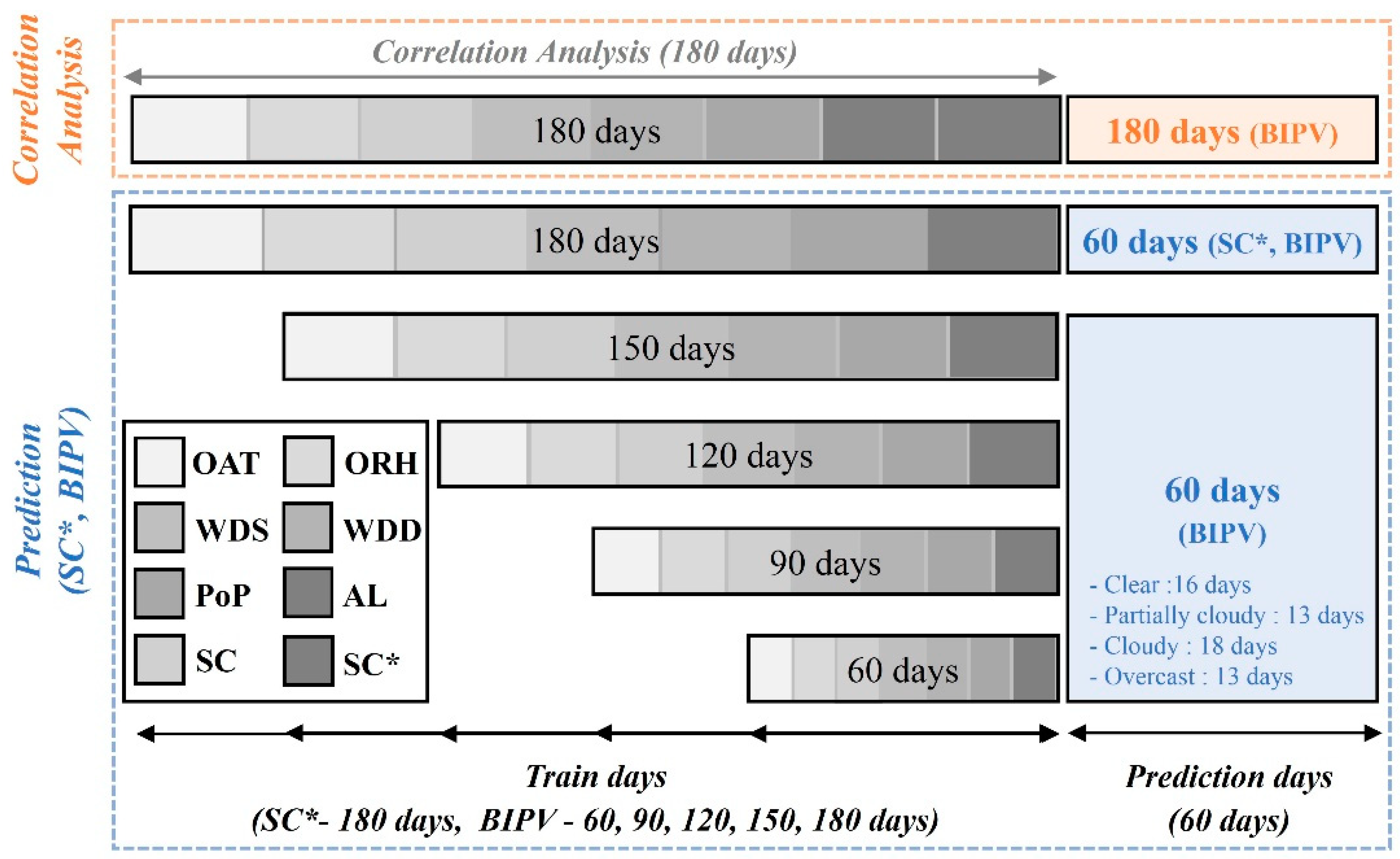
The on-site database management system of BEMS has collected the hourly weather forecast data and BIPV power output since June 2022. The model can use the last six months (180 days) of hourly data for training (from December 2022 to May 2023). The prediction started on June 1st and ended on July 2023 for 60 days without two days of missing data.

2.5. Performance Evaluation Indices

MAPE and R² in Equations (4) and (5) evaluated the model performance for estimating the hourly SC* and BIPV power output a day ahead.

$$MAPE=\frac{1}{n}\times {\sum }_{t=1}^n\left|\frac{P_t-A_t}{A_t}\right|\times 100(\%)$$

(4)

$$R^2=\frac{{[\sum _{t=1}^n{(P}_t-{\overline{P}}_t)·{(A}_t-{\overline{A}}_t)]}^2}{[\sum _{t=1}^n{(P}_t-{\overline{P}}_t)·{(A}_t-{\overline{A}}_t)]}$$

(5)

where $A_t$ and $P_t$ are the actual and predicted values, respectively; $A_t$ and $P_t$ are the mean values of ${\overline{A}}_t$ and ${\overline{P}}_t$, respectively; and n is the number of data. The MAPE evaluates the hourly prediction performance of SC* and BIPV power output. The R² determines the level of linear relationships between the predicted and actual values. The lower MAPE indicates the higher accuracy of the model, and vice versa in the case of R² [50,51].

3. Results and Analysis

The day-ahead BIPV power output prediction model has three phases, as shown in Figure 4. First, it conducted the correlation analysis for 180 days between weather forecast features with a new feature (modified sky condition, SC*) and BIPV power output over time. Then, the model predicted the day-ahead hourly SC* using the weather dataset from the forecasting service. At last, the performance evaluation of the hourly BIPV power output predictions with different model conditions for 60 days.

3.1. Derivation of New Feature

The KMA only provides a natural number code in the normative SC (Clear-1, Partially Cloudy-2, Cloudy-3, and Overcast-4) for three hours. When the sky conditions are 3 at a time step, for example, the sky would be cloudy for three hours until the next forecasting service. It may result in almost the same PV power output for the period.

This study proposed a new synthetic feature, SC* (modified sky condition), which can describe on-site sky conditions with real numbers from −5.0 to + 5.0 hourly using a feature engineering method. First, a Pearson correlation method was employed to identify the correlation coefficient of the seven factors to evaluate their correlation with the hourly BIPV power output [52]. The correlation method is expressed in Equation (6).

$$\gamma =\frac{n\left(\sum w_i{p}_i\right)-\left(\sum w_i\right)·\left(\sum p_i\right)}{\sqrt{\left(n\sum w_i^2-{\left(\sum w_i\right)}^2\right)}·\left(n\sum p_i^2-{\left(\sum p_i\right)}^2\right)}$$

(6)

where γ is the correlation coefficient, $w_i$ is the input features, $p_i$ is the target parameter (BIPV power output), and n is the number of data.

Second, the calculated SC* was obtained by correlating the hourly AL and actual BIPV power output (PV). The hourly AL shows regular periodic patterns regardless of the weather condition, but the hourly BIPV power output changes with the on-site weather conditions. The calculated SC* can define the ratio of variables in BIPV power output, denoted ∆P, and solar altitude angle, denoted ∆S, between current and previous time steps, as expressed in Equation (7).

$${{SC}^{*}}_{\left(t\right)}=\frac{∆P}{∆S}=\frac{{PV}_{\left(t\right)}-{PV}_{\left(t-1\right)}}{\left|{Al}_{\left(t\right)}-{Al}_{(t-1)}\right|}$$

(7)

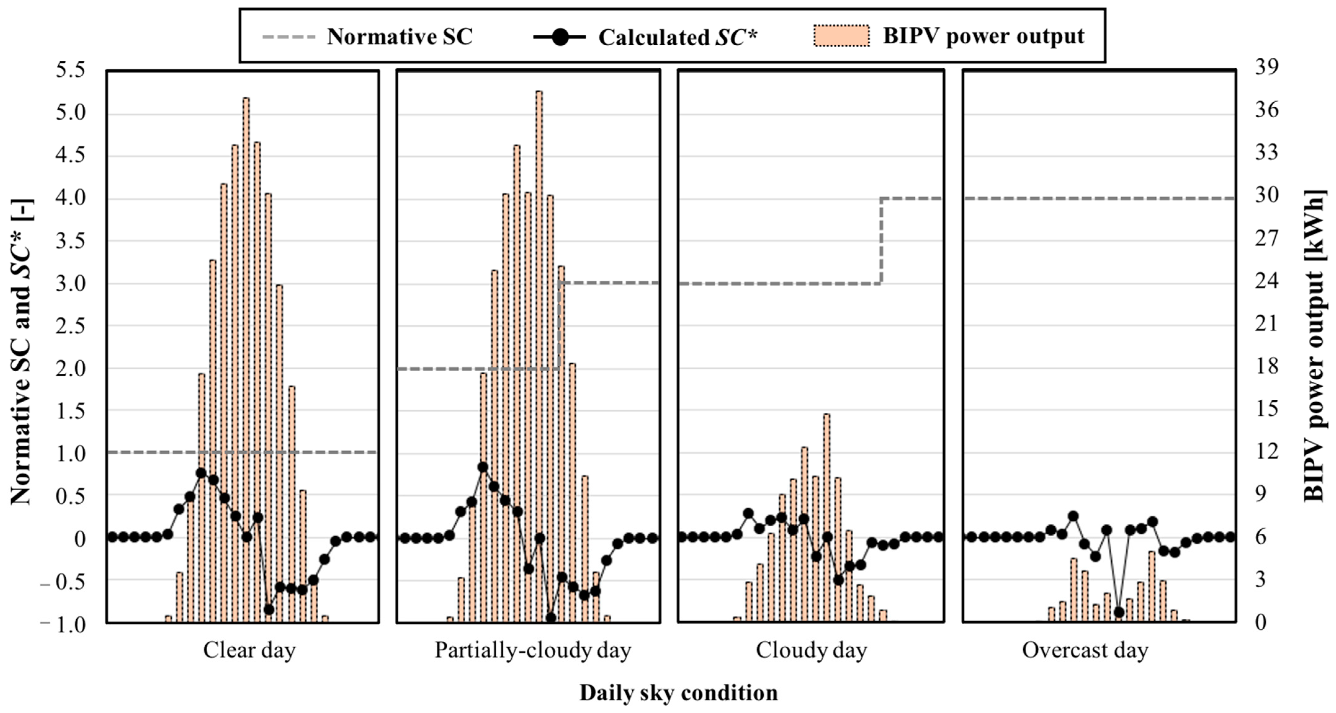
where PV and AL are the hourly power output and the solar altitude angle in the current (t) and the previous time step (t – 1), respectively. The value will be positive when the sky is clear, whereas it will be negative if the current BIPV power output is less than the value of the previous time step until noon. In the afternoon, calculated SC* will have a negative value, but it will be significantly lower when the clouds cast a shadow on the BIPV, as shown in Figure 5. Hourly SC* values are more sensitive to the normative SC from the forecasting service compared to the hourly BIPV power output. On day 2 in Figure 5, the normative SC was constant each time, whereas the BIPV power output was not as steady as the normative sky condition.

Since the calculated hourly SC* is derived from past hourly BIPV power output and solar altitude, it is necessary to have predictions on hourly SC* using weather forecast data and AL. Thereafter, the predicted SC* can be inputted into the BIPV power output prediction model as an input feature.

3.2. Characteristics of BIPV Power Output

Table 6. Correlation coefficient of each weather feature with hourly PV power output (4320 h).

	$\mathbf{O}\mathbf{A}\mathbf{T}$	$\mathbf{O}\mathbf{R}\mathbf{H}$	$\mathbf{W}\mathbf{D}\mathbf{S}$	$\mathbf{W}\mathbf{D}\mathbf{D}$	$\mathbf{P}\mathbf{o}\mathbf{P}$	$\mathbf{A}\mathbf{L}$	$\mathbf{S}\mathbf{C}$	${\mathbf{S}\mathbf{C}}^{\mathbf{*}}$
Correlation coefficient	+0.48	−0.56	+0.04	+0.05	−0.22	+0.82	−0.22	+0.42

$\mathrm{A}\mathrm{L}$ was hourly original data, ${\mathrm{S}\mathrm{C}}^{\mathrm{*}}$ was calculated.

shows the correlation results between the preprocessed features in Table 4 and the on-site hourly BIPV power output during the total 4320 h and 180 days (December 2022 to May 2023). It revealed that the hourly solar position (AL) had the highest correlation with the hourly BIPV power output (r = +0.82). In addition, ORH (r = −0.61) and OT (r = +0.52) showed the second-highest correlation. Compared to SC (r = −0.22), SC* (r = +0.42) showed a stronger correlation with the BIPV power output. For SC, significantly decoupled with the daily total BIPV power output, the correlation value was almost similar to the PoP (r = −0.22), although it would be a fundamental classifier to infer the solar irradiation level.

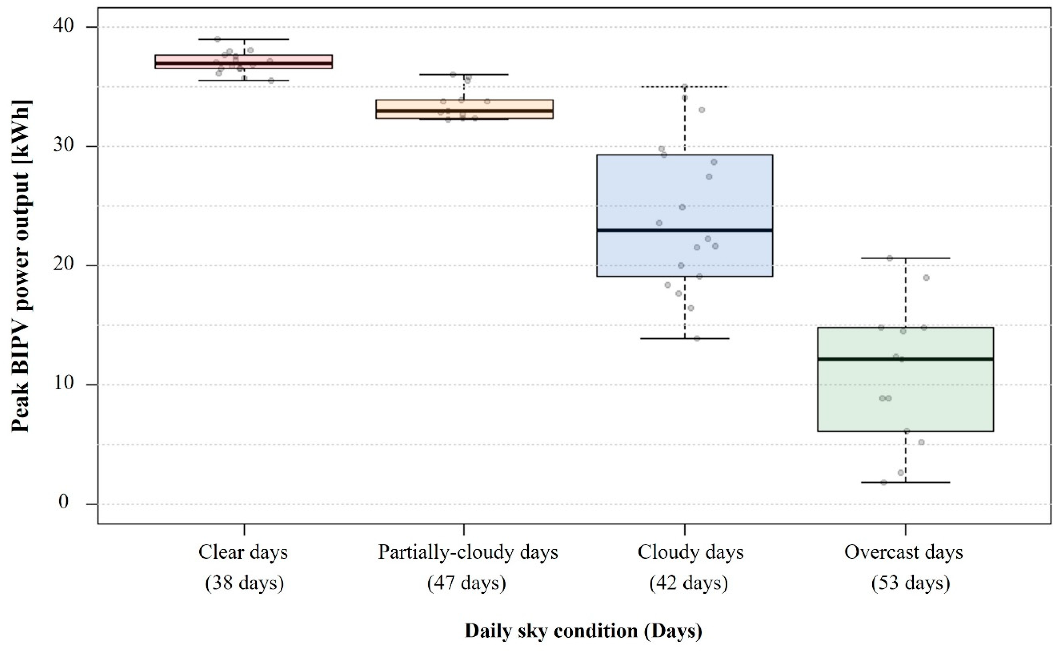
Figure 6 shows the daily peak PV power output under different daily-averaged sky conditions, Clear, Partially Cloudy, Cloudy, and Overcast, from the weather forecasting service. On Clear and Partially Cloudy days (85 days), the daily peak PV power output had lower deviations than the peak powers of Cloudy and Overcast days (95 days). The daily peak power outputs range from 32.27 kWh to 38.95 kWh, but the uncertainty of power output highly increases on Overcast days, ranging from 1.82 kWh to 20.59 kWh.

These results may illustrate two main drawbacks to harnessing the normative SC for PV power output prediction. First, a single natural number for this three-hour with 5 × 5 km geometrical resolution does not represent the hourly on-site sky condition. In addition, the scale of the SC (i.e., four steps in an integer) may not correlate with the hourly variance of the power output value.

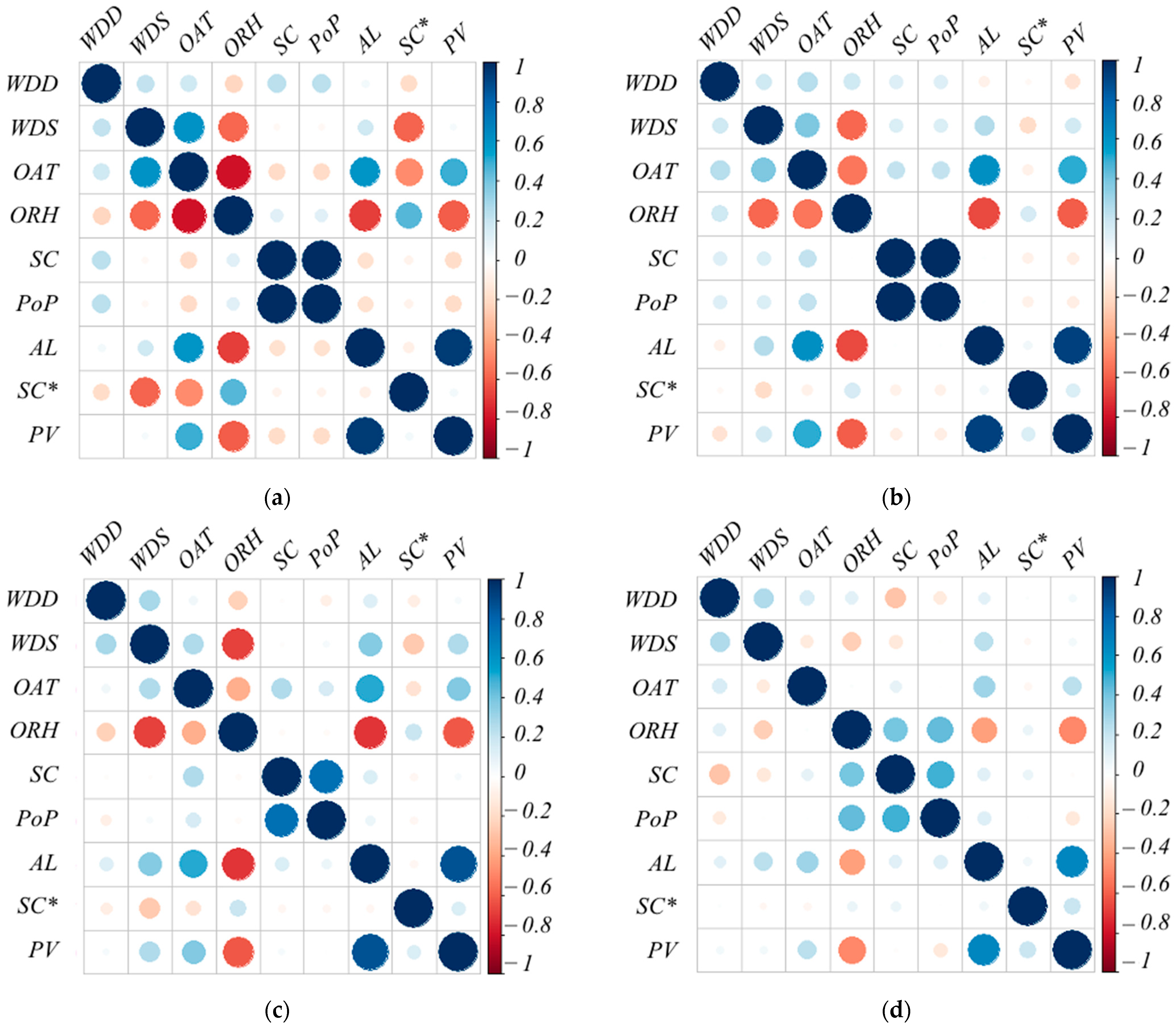
Figure 7 illustrates the coefficient of correlation for each feature under different daily-averaged sky conditions for the test period. AL, ORH, and OAT were the most correlated variables with the PV power output on most days. In addition, the hourly normative SC placed 4th on clear days and 7th on other days. It means the variance of the SC had no effect on the hourly BIPV power outputs except on Clear days. Whereas, a new derivate value, SC*, placed sixth on Clear and Partially Cloudy days, but it had a stronger correlation to PV power output than the normative SC on Cloudy and Overcast days. The correlation coefficient of SC* increased from +0.04 on Clear days to +0.22 on Overcast days. Furthermore, normative SC shows a lower correlation with PoP as the sky becomes cloudier. This is because the normative SC has a constant value in Cloudy and Overcast days, but the PoP has higher scalability compared to the normative SC.

Figure 8 shows each hourly SC, SC*, and BIPV power output under typical sky conditions. SC cannot reflect the hourly BIPV power output change over time since the value is constant for three hours. However, the new feature, SC*, varied with time and hourly BIPV power output.

The analysis illustrates that the newly developed feature, SC*, is correlated with hourly BIPV power output under all different criteria, including the total test periods (180 days), the daily averaged sky conditions, and the hourly variations of typical days.

3.3. Day-Ahead SC* Predictions

It is necessary to conduct the hourly SC* predictions using the NARX network described in the previous section using the past forecasted weather and calculated SC*, which has hourly relationships between AL and BIPV power output generation.

Using the past data of the 180 days from December 2022 to May 2023, the NARX model predicted the day-ahead hourly SC* from 1 June to 31 July 2023 (60 days) with a daily sliding window approach that updates the training set on a day.

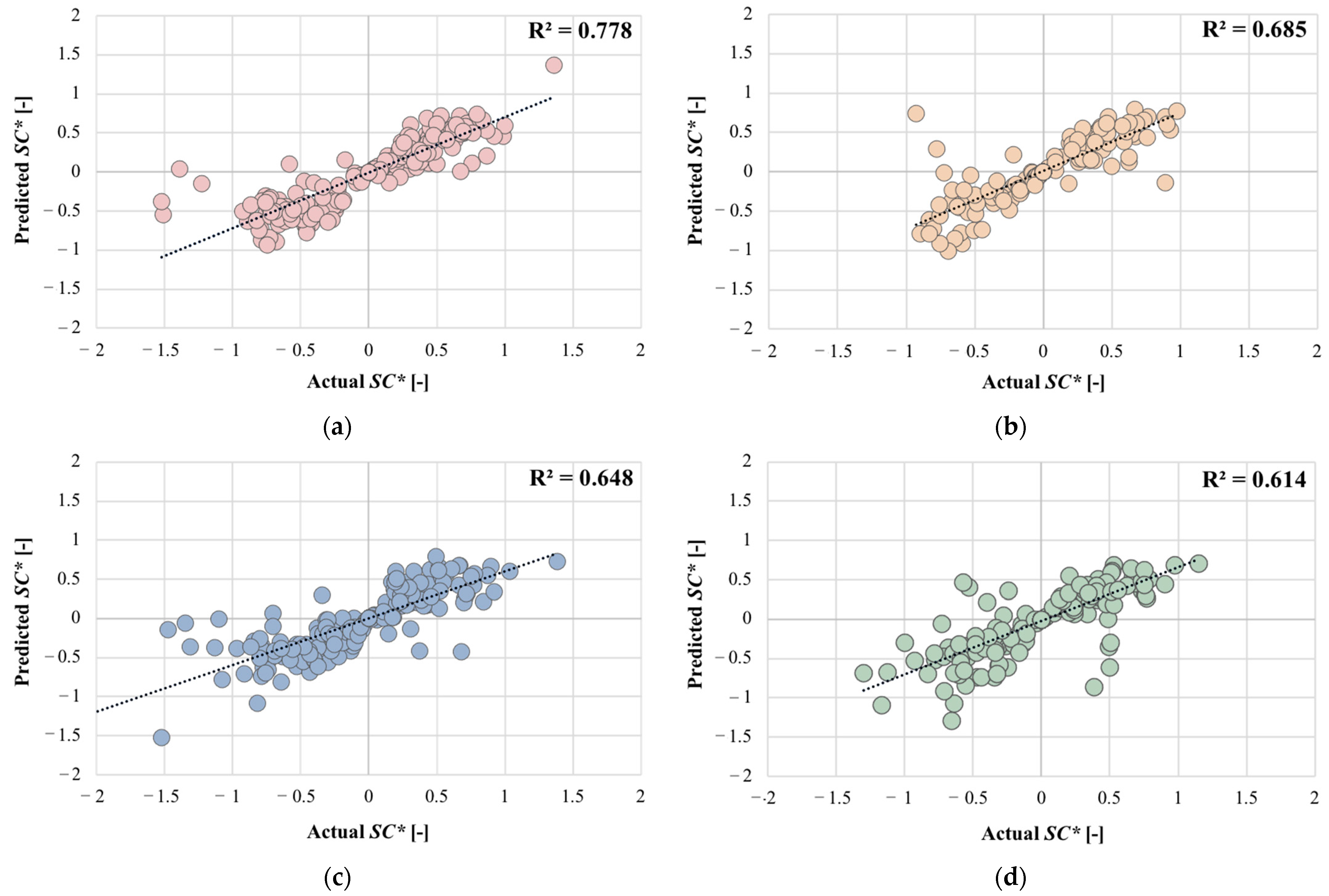
Figure 9 compares the hourly calculated SC* and predicted SC*. As illustrated in the previous section, the calculated SC* is derived from past weather data and BIPV outputs, but the predicted SC* is an output of the NARX model using the solar position and weather forecasting data. For 60 days, the predicted SC* showed a higher value of R² with the calculated value on Clear (R² = 0.778) and Partially Cloudy (R² = 0.685) days. The performance degraded on Cloudy (R² = 0.648) and Overcast days (R² = 0.614).

The average MAPE value of the hourly predicted SC* for the 60 days under four daily averaged sky conditions was 20.07%, as illustrated in

Table 7. Performance evaluation for predicted ${SC}^{*}$ with different sky conditions.

Daily Sky Condition	Days	MAPE (%)	R2
Clear days	16	17.20	0.778
Partially cloud days	13	17.91	0.685
Cloudy days	18	23.64	0.648
Overcast days	13	21.52	0.614

. The highest prediction performance of SC* was observed on clear days (16 days), with a MAPE value of 17.20%. On Partially Cloudy days (13 days), Cloudy days (18 days), and Overcast days (13 days), the MAPE values were 17.91, 23.64, and 21.52%, respectively. Figure 10 compares the predicted hourly SC* with the calculated SC* under typical daily averaged sky conditions. Although the NARX model lost accuracy somewhat on Cloudy and Overcast days, the predicted SC* values had a similar hourly pattern to the calculated SC* value in most sky conditions.

3.4. Performance BIPV Power Output Prediction Model under Different Model Configurations

3.4.1. Selection of Training Size

As described in the previous section, the hourly BIPV power output varied with a change in the onsite weather, sky conditions, and dynamics of solar position according to the time of day and season. Generally, the size of the training data is essential for a machine-learning approach. As the model reconstructs the weight and bias using past data sets, the quality and quantity of the training data significantly affect the model performance.

Regarding the quality of the past data, the data processing managed the missing data and outliers. Linear interpolation converted 3 hours of past weather forecasted data to an hour. To define the optimized training data set, the model performance for the day-ahead prediction of BIPV power output for 60 days using the weather forecasting indices without SC* was evaluated using different training sets under the same model hyperparameter configurations.

Table 8. The evaluated days for BIPV power output with daily sky conditions.

Days	Days (Proportion)
	Clear	Partially Cloudy	Cloudy	Overcast
60 days	11 days (18%)	33 days (55%)	11 days (18%)	5 days (8%)
90 days	21 days (23%)	45 days (50%)	14 days (16%)	10 days (11%)
120 days	34 days (28%)	52 days (43%)	21 days (18%)	13 days (11%)
150 days	42 days (28%)	58 days (39%)	31 days (21%)	19 days (13%)
180 days	47 days (26%)	66 days (37%)	42 days (23%)	25 days (14%)

illustrates the ratio of each daily average sky condition to the potential training size (60, 90, 120, 150, and 180 days).

Figure 11 compares the model performance for the hourly BIPV power output predictions under four typical sky conditions with different training sizes. On Clear days, the MAPE values ranged from 8.54 (120 days) to 10.17% (180 days). On Partially Cloudy days, the MAPE increased from 11.55 (90 days) to 23.25% (60 days). The 90 days of training data were suitable for the model performance among the potential training sizes, especially on Cloudy (21.33%) and Overcast (54.64%) days.

Although the prediction model performance would not depend on training size on Clear days, the model with 90 days of training outperformed other training size cases on Partially Cloudy, Cloudy, and Overcast days. Therefore, this study investigated the model performance using 90 days of training.

3.4.2. Sensitivity of Predictors

It is necessary to assess the feasibility of the pre-determined training size and the predicted SC* as a predictor. The NARX network model with the typical model configuration in Table 4 predicted the day-ahead hourly BIPV power output under different input conditions from June to July 2023 (60 days), as described in

Table 9. Input condition for day-ahead prediction of BIPV power output.

	Baseline	Case 1	Case 2	Case 3	Case 4
OAT	√	√	√	√	√
ORH	√	√	√	√	√
WDS	√	√	√	-	-
WDD	√	√	√	-	-
PoP	√	√	√	-	-
AL	√	√	√	√	-
SC	√	√	-	-	-
${SC}^{*}$	-	√	√	√	√

√: Included, -: Not included.

. Five predictor conditions are as follows: Baseline: only the weather forecasted indices with AL; Case-1: added the predicted SC* into Baseline; Case-2: removed the normative SC from Case-1; Case-3: removed WDD, WDS, and PoP from Case-2; and Case-4: using OAT, ORH, and SC* only.

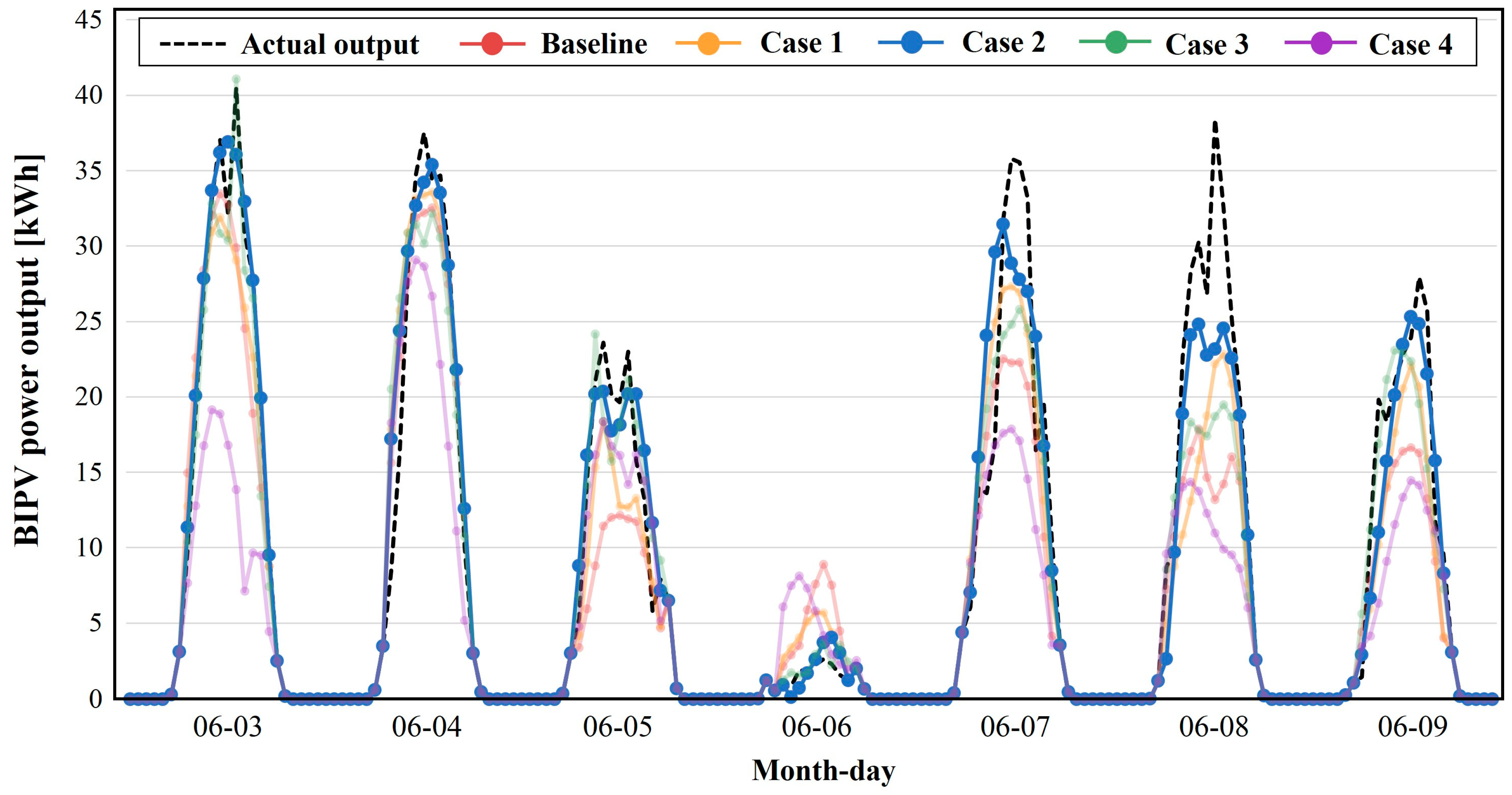
Figure 12 shows time series data of the model prediction performance for the first week, seven days, of the actual prediction under the different input cases. Under Base, the prediction performances on Clear days (6/3–6/4) were highly accurate with 8.51% and 8.03% in MAPE. The model performance was not well on Partially Cloudy days (6/7–6/9) with MAPE values of 13.60%, 16.39%, and 22.96%, respectively. The lowest accuracy was observed on Cloudy (6/7) and Overcast (6/8) days.

In Case-1, which included all the predictors and the predicted SC*, the performance of the model was higher than that under Base, particularly on Partially Cloudy days with lower MAPE ranges of 14.33 (6/7), 15.94 (6/8), and 16.39% (6/9). The performance of the model on Cloudy and Overcast days (6/5~6/6) was similar to that under Base.

When the predicted SC* was substituted for the normative SC, Case-2 showed the highest accuracy of the actual power output prediction. The MAPE of the hourly BIPV power output (168 h) for seven days (6/3–6/9) was 11.39%. On Clear days, the MAPE values were 2.67 (6/3) and 8.77% (6/4). The value ranged from 9.25 (6/8) to 13.24% (6/7) on Partially Cloudy days. Although the MAPE values on Cloudy (11.95%, 6/5) and Overcast (16.39%, 6/6) days were higher than those on Clear and Partially Cloudy days, the performances of the model under these conditions were better than those under other input conditions. In addition, compared to other cases, there was a better agreement with the daily peak of BIPV power generation on most days. The predicted SC* may provide the actual onsite sky condition better than the normative SC.

When the WDD, WDS, and PoP, which are the lower correlation coefficient predictors in the previous section, were removed from the predictors in Case-3, the MAPE of the total period was 13.33%, which was 2% higher than that of Case-2, but the hourly BIPV power output pattern was closed to Case-2. It may illustrate that the low correlation coefficient predictors do not affect improving model performance.

The effects of the higher correlation coefficient predictors on the model performance were explicit in Case-4. When ORH, OAT, and SC* only were used as the predictors, and AL, which is the most correlated predictor among the input features, was removed, the model yielded the worst performance compared to other input conditions. Under this condition, the MAPE value of the total period was 39.02%. Although the model performance on cloudy days (MAPE = 12.14%) has similar performances in other cases, the MAPE value on Overcast days was above 100%.

3.5. Long-Term Model Performance Tracking

The model performance under the five input conditions (Base~Case-4) was evaluated through long-term testing for 60 days (June and July 2023), as illustrated in Figure 13 and

Table 10. Overall performance of BIPV power output with different input conditions.

Daily Sky Condition (Days)	MAPE (R2)
	Base	Case 1	Case 2	Case 3	Case 4
Clear (16 days)	9.33% (0.98)	8.92% (0.98)	6.12% (0.99)	10.72% (0.97)	23.22% (0.92)
Partially Cloudy (13 days)	11.55% (0.95)	9.54% (0.97)	10.20% (0.95)	12.08% (0.95)	18.78% (0.88)
Cloudy (18 days)	21.33% (0.84)	17.31% (0.90)	16.53% (0.92)	16.89% (0.93)	27.51% (0.82)
Overcast (13 days)	54.64% (0.76)	53.16% (0.85)	27.70% (0.93)	33.05% (0.85)	42.24% (0.77)

.

Under Base, the model achieved an overall MAPE of 24.21% and R² of 0.88. The predicted BIPV power output of the model under this condition on Clear days (16 days) and Partially Cloudy days (13 days) was close to the actual power output on these days, with the averaged MAPE of 10.44% and the averaged R² of 0.97. However, the accuracy and correlation on Cloudy days (18 days) degraded as the MAPE value increased to 21.33% and the R² decreased to 0.83. The prediction accuracy decreased on Overcast days (13 days) as the MAPE value increased to 54.64% and the R² decreased to 0.76. It resulted in a similar performance to the hourly data of a typical week-time series illustrated in Figure 11.

When the model adopted the hourly predicted SC* as a predictor (Case-1), the additional input improved the model performance, with an average MAPE of 22.23% and R² of 0.93 in the period. Compared to the Base, the model accuracy on Clear and Partially Cloudy days was slightly enhanced (by MAPE values of 0.41 and 2.01%, respectively). In particular, the input condition improved the model performance on Cloudy days (MAPE = 17.31%, R² = 0.90) and Overcast days (MAPE = 53.16%, R² = 0.85).

Under Case-2, the model performance was higher than those under other input conditions, as the typical week analysis with the average 60-day MAPE of 15.14% and R² of 0.95. Compared to Base, this input condition provided the highest accuracy as the MAPE values decreased by 3.21, 1.35, and 4.80% on Clear, Partially Cloudy, and Cloudy days, respectively. The MAPE and R² on Overcast days were 27.70% and 0.93, corresponding to an increase of 49.30% and 0.18, respectively, compared to that of Base. Compared to [29], which uses only the weather forecast data set, the suggested process can improve the prediction performance by 3.88% in MAPE under Clear days and 52.37% in MAPE under Cloudy days.

Under Case-3, the average MAPE and R² of the overall period were 18.19% and 0.93, respectively. Although the MAPE and R² on Clear and Partially Cloudy days were similar to those of Base and Case-1, the model performance on Cloudy and Overcast days under this condition was better than those of the former two cases. Compared to Case-2, the results indicated that the model showed consistent performance except on Overcast days, even if the model used simple predictors. It may illustrate that the lower correlated coefficient variable functioned as redundant variables to predict the BIPV power outputs in Base and Case-1.

Under Case-4, the model showed the worst performance on most days compared to other input conditions. The average MAPE and R² were 27.94% and 0.85, respectively. The results of Case-3 and Case-4 supported two points. First, BIPV prediction using only the weather forecast data may be insufficient for achieving acceptable performance. Second, the data pre-processing can identify the essential variables (i.e., AL and SC*) that can subsequently improve the BIPV power output prediction performance.

4. Conclusions

This study presents a feasible approach to predicting a day-ahead hourly BIPV power output with a simple weather forecasting service that does not provide the forecasting of solar irradiation. With a new parameter, the modified sky condition (SC*), developed through feature engineering and a simple machine learning model, the suggested approach yields acceptable prediction accuracy and stable model performance in four different sky conditions.

The developed model involved two stages of prediction. First, the NARX model predicts hourly SC* with the stored weather data and PV power outputs, then the model predicts hourly BIPV power output using the real-time weather forecasting service data, predicted SC*, and solar altitude of the site.

Although the predicted hourly SC* was consistent at approximately 20% in MAPE during the prediction period with four different daily sky conditions, the hourly pattern was more similar to the hourly PV power output than the normative SC in the weather forecast service.

The input feature sensitivity analysis showed that the model accuracy was significantly improved when the predicted SC* and AL replaced the normative SC. With long-term performance tracking for 60 days, the model yielded an overall MAPE and R² of 15.14% and 0.95, respectively. The new features enhanced the prediction accuracy by 36% on average, especially on Cloudy (18 days) and Overcast (13 days) sky conditions compared with the model performance with conventional weather forecasting service data.

Since it does not require installing an on-site weather station with a pyranometer and Database to store the weather station data, it can reduce the implementation cost and time for a new BIPV on buildings. For BIPV in existing buildings, the model can be available immediately as long as BMS (Building Management System) has hourly PV outputs longer than 90 days for the training data set.

This study used a typical NARX model to select the training size and predict hourly SC* and PV power output a day ahead. The performance evaluation with the other models, which have different model complexities and training conditions, will be necessary to improve the capabilities of the suggested process. In addition, it needs to be generalized by applying it to other buildings. Further, it is necessary to optimize PV power outputs, electric storage, and building energy demand to improve building energy management and reduce greenhouse gas emissions from buildings.

References

1. Furukakoi, M.; Adewuyi, O.B.; Matayoshi, H.; Howlader, A.M.; Senjyu, T. Multi objective unit commitment with voltage stability and PV uncertainty. Appl. Energy 2018, 228, 618–623. [Google Scholar] [CrossRef]
2. Gallardo, I.; Amor, D.; Gutiérrez, Á. Recent Trends in Real-Time Photovoltaic Prediction Systems. Energies 2023, 16, 5693. [Google Scholar] [CrossRef]
3. Nunes, H.G.G.; Pombo, J.A.N.; Mariano, S.J.P.S.; Calado, M.R.A.; De Souza, J.F. A new high performance method for determining the parameters of PV cells and modules based on guaranteed convergence particle swarm optimization. Appl. Energy 2018, 211, 774–791. [Google Scholar] [CrossRef]
4. Elum, Z.A.; Momodu, A.S. Climate change mitigation and renewable energy for sustainable development in Nigeria: A discourse approach. Renew. Sustain. Energy Rev. 2017, 76, 72–80. [Google Scholar] [CrossRef]
5. Gao, H.; Wang, X.; Wu, K.; Zheng, Y.; Wang, Q.; Shi, W.; He, M. A review of building carbon emission accounting and prediction models. Buildings 2023, 13, 1617. [Google Scholar] [CrossRef]
6. Yu, K.; Liang, J.J.; Qu, B.Y.; Cheng, Z.; Wang, H. Multiple learning backtracking search algorithm for estimating parameters of photovoltaic models. Appl. Energy 2018, 226, 408–422. [Google Scholar] [CrossRef]
7. Gassar, A.A.A.; Cha, S.H. Review of geographic information systems-based rooftop solar photovoltaic potential estimation approaches at urban scales. Appl. Energy 2021, 291, 116817. [Google Scholar] [CrossRef]
8. Ghaithan, A.M.; Mohammed, A.; Al-Hanbali, A.; Attia, A.M.; Saleh, H. Multi-objective optimization of a photovoltaic-wind-grid connected system to power reverse osmosis desalination plant. Energy 2022, 251, 123888. [Google Scholar] [CrossRef]
9. Sun, T.; Shan, M.; Rong, X.; Yang, X. Estimating the spatial distribution of solar photovoltaic power generation potential on different types of rural rooftops using a deep learning network applied to satellite images. Appl. Energy 2022, 315, 119025. [Google Scholar] [CrossRef]
10. International Energy Agency (IEA). Renewables 2017- Executive summary. International Energy Agency (IEA). 2017. Available online: www.iea.org (accessed on 18 July 2023).
11. Shi, K.; Li, C.; Koo, C. A Techno-Economic Feasibility Analysis of Mono-Si and Poly-Si Photovoltaic Systems in the Rooftop Area of Commercial Building under the Feed-In Tariff Scheme. Sustainability 2021, 13, 4709. [Google Scholar] [CrossRef]
12. Gawley, D.; McKenzie, P. Investigating the suitability of GIS and remotely-sensed datasets for photovoltaic modelling on building rooftops. Energy Build. 2022, 265, 112083. [Google Scholar] [CrossRef]
13. Pillai, D.S.; Shabunko, V.; Krishna, A. A comprehensive review on building integrated photovoltaic systems: Emphasis to technological advancements, outdoor testing, and predictive maintenance. Renew. Sustain. Energy Rev. 2022, 156, 111946. [Google Scholar] [CrossRef]
14. Liu, J.; Zhou, Y.; Yang, H.; Wu, H. Net-zero energy management and optimization of commercial building sectors with hybrid renewable energy systems integrated with energy storage of pumped hydro and hydrogen taxis. Appl. Energy 2022, 321, 119312. [Google Scholar] [CrossRef]
15. Hasan, J.; Fung, A.S.; Horvat, M. A comparative evaluation on the case for the implementation of building integrated photovoltaic/thermal (BIPV/T) air based systems on a typical mid-rise commercial building in Canadian cities. J. Build. Eng. 2021, 44, 103325. [Google Scholar] [CrossRef]
16. Raza, M.Q.; Nadarajah, M.; Ekanayake, C. Demand forecast of PV integrated bioclimatic buildings using ensemble framework. Appl. Energy 2017, 208, 1626–1638. [Google Scholar] [CrossRef]
17. Li, Y.; Liu, C. Techno-economic analysis for constructing solar photovoltaic projects on building envelopes. Build. Environ. 2018, 127, 37–46. [Google Scholar] [CrossRef]
18. Fekkak, B.; Menaa, M.; Boussahoua, B. Control of transformerless grid-connected PV system using average models of power electronics converters with MATLAB/Simulink. Sol. Energy 2018, 173, 804–813. [Google Scholar] [CrossRef]
19. Kuhn, T.E.; Erban, C.; Heinrich, M.; Eisenlohr, J.; Ensslen, F.; Neuhaus, D.H. Review of technological design options for building integrated photovoltaics (BIPV). Energy Build. 2021, 231, 110381. [Google Scholar] [CrossRef]
20. Park, H. A Stochastic Planning Model for Battery Energy Storage Systems Coupled with Utility-Scale Solar Photovoltaics. Energies 2021, 14, 1244. [Google Scholar] [CrossRef]
21. Zhang, Y.; Vand, B.; Baldi, S. A Review of Mathematical Models of Building Physics and Energy Technologies for Environmentally Friendly Integrated Energy Management Systems. Buildings 2022, 12, 238. [Google Scholar] [CrossRef]
22. Netsanet, S.; Zheng, D.; Zhang, J.; Hui, M. Predictors Selection and Accuracy Enhancement Techniques in PV Forecasting Using Artificial Neural Network. In Proceedings of the IEEE International Conference on Power and Renewable Energy, Melaka, Malaysia, 21–23 October 2016. [Google Scholar] [CrossRef]
23. Abdel-Nasser, M.; Mahmoud, K. Accurate photovoltaic power forecasting models using deep LSTM-RNN. Neural Comput. Appl. 2019, 31, 2727–2740. [Google Scholar] [CrossRef]
24. Li, Y.; He, Y.; Su, Y.; Shu, L. Forecasting the daily power output of a grid-connected photovoltaic system based on multivariate adaptive regression splines. Appl. Energy 2016, 180, 392–401. [Google Scholar] [CrossRef]
25. Chiang, P.H.; Chiluvuri, S.P.V.; Dey, S.; Nguyen, T.Q. Forecasting of solar photovoltaic system power generation using wavelet decomposition and bias-compensated random forest. In Proceedings of the 2017 Ninth Annual IEEE Green Technologies Conference (GreenTech), Denver, CO, USA, 29–31 March 2017; pp. 260–266. [Google Scholar] [CrossRef]
26. Ramsami, P.; Oree, V. A hybrid method for forecasting the energy output of photovoltaic systems. Energy Convers. Manag. 2015, 95, 406–413. [Google Scholar] [CrossRef]
27. Tang, Y.; Yang, K.; Zhang, S.; Zhang, Z. Photovoltaic power forecasting: A hybrid deep learning model incorporating transfer learning strategy. Renew. Sustain. Energy Rev. 2022, 162, 112473. [Google Scholar] [CrossRef]
28. Abou Houran, M.; Bukhari, S.M.S.; Zafar, M.H.; Mansoor, M.; Chen, W. COA-CNN-LSTM: Coati optimization algorithm-based hybrid deep learning model for PV/wind power forecasting in smart grid applications. Appl. Energy 2023, 349, 121638. [Google Scholar] [CrossRef]
29. Nespoli, A.; Ogliari, E.; Leva, S.; Massi Pavan, A.; Mellit, A.; Lughi, V.; Dolara, A. Day-ahead photovoltaic forecasting: A comparison of the most effective techniques. Energies 2019, 12, 1621. [Google Scholar] [CrossRef]
30. Monfared, M.; Fazeli, M.; Lewis, R.; Searle, J. Day-ahead prediction of pv generation using weather forecast data: A case study in the UK. In Proceedings of the 2020 International Conference on Electrical, Communication, and Computer Engineering (ICECCE), Istanbul, Turkey, 12–13 June 2020; pp. 1–5. [Google Scholar] [CrossRef]
31. Polasek, T.; Čadík, M. Predicting photovoltaic power production using high-uncertainty weather forecasts. Appl. Energy 2023, 339, 120989. [Google Scholar] [CrossRef]
32. Korea Meteorological Administration. Meteorological Data Open Portal (in Korean). Available online: https://data.kma.go.kr/cmmn/main.do (accessed on 15 June 2023).
33. Korea Meteorological Administration. A Study on the Diagnosis and Development Direction of the Forecasting System; Korea Meteorological Administration: Seoul, Republic of Korea, 2019.
34. Encyclopedia of Mathematics. Linear interpolation. Available online: https://encyclopediaofmath.org/wiki/Linear_interpolation (accessed on 20 June 2022).
35. Yang, S. Feature Engineering in Fine-Grained Image Classification. Ph.D. Thesis, University of Washington, Seattle, WA, USA, July 2013. Available online: http://hdl.handle.net/1773/23376 (accessed on 3 October 2023).
36. Cadenas, E.; Rivera, W.; Campos-Amezcua, R.; Heard, C. Wind speed prediction using a univariate ARIMA model and a multivariate NARX model. Energies 2016, 9, 109. [Google Scholar] [CrossRef]
37. Andalib, A.; Atry, F. Multi-step ahead forecasts for electricity prices using NARX: A new approach, a critical analysis of one-step ahead forecasts. Energy Convers. Manag. 2009, 50, 739–747. [Google Scholar] [CrossRef]
38. Katić, K.; Li, R.; Verhaart, J.; Zeiler, W. Neural network based predictive control of personalized heating systems. Energy Build. 2018, 174, 199–213. [Google Scholar] [CrossRef]
39. Siegelmann, H.T.; Horne, B.G.; Giles, C.L. Computational capabilities of recurrent NARX neural networks. IEEE Trans. Syst. Man Cybern. Part B 1997, 27, 208–215. [Google Scholar] [CrossRef] [PubMed]
40. Fleifel, R.T.; Soliman, S.S.; Hamouda, W.; Badawi, A. LTE primary user modeling using a hybrid ARIMA/NARX neural network model in CR. In Proceedings of the 2017 IEEE Wireless Communications and Networking Conference (WCNC), San Francisco, CA, USA, 19–22 March 2017; pp. 1–6. [Google Scholar] [CrossRef]
41. Eugen, D. The use of NARX Neural Networks to predict Chaotic Time Series. Wseas Trans. Comput. Res. 2008, 3, 182–191. [Google Scholar]
42. Sansa, I.; Missaoui, S.; Boussada, Z.; Bellaaj, N.M.; Ahmed, E.M.; Orabi, M. PV power forecasting using different artificial neural networks strategies. In Proceedings of the 2014 First International Conference on Green Energy ICGE, Sfax, Tunisia, 25–27 March 2014; pp. 54–59. [Google Scholar] [CrossRef]
43. Argyropoulos, D.; Paraforos, D.S.; Alex, R.; Griepentrog, H.W.; Müller, J. NARX neural network modelling of mushroom dynamic vapour sorption kinetics. IFAC-PapersOnLine 2016, 49, 305–310. [Google Scholar] [CrossRef]
44. Çoruh, S.; Geyikçi, F.; Kılıç, E.; Çoruh, U. The use of NARX neural network for modeling of adsorption of zinc ions using activated almond shell as a potential biosorbent. Bioresour. Technol. 2014, 151, 406–410. [Google Scholar] [CrossRef] [PubMed]
45. Jose, M.P.J.; Guilherme, A.B. Multistep-Ahead Prediction of Rainfall Precipitation Using the NARX Network. In Proceedings of the European Symposium on Time Series Prediction, ESTSP 2008, Porvoo, Finland, 17–19 September 2008. [Google Scholar]
46. Liu, H.; Song, X. Nonlinear system identification based on NARX network. In Proceedings of the 2015 10th Asian Control Conference (ASCC), Kota Kinabalu, Malaysia, 31 May–3 June 2015; pp. 1–6. [Google Scholar] [CrossRef]
47. Bektas, O.; Jones, J.A. NARX time series model for remaining useful life estimation of gas turbine engines. In Proceedings of the PHM Society European Conference 2016, Bilbao, Spain, 5–8 June 2016; Volume 3. [Google Scholar]
48. Koç, C.K. Analysis of sliding window techniques for exponentiation. Comput. Math. Appl. 1995, 30, 17–24. [Google Scholar] [CrossRef]
49. Menezes, J.M.P., Jr.; Barreto, G.A. Long-term time series prediction with the NARX network: An empirical evaluation. Neurocomputing 2008, 71, 3335–3343. [Google Scholar] [CrossRef]
50. Goodwin, P.; Lawton, R. On the asymmetry of the symmetric MAPE. Int. J. Forecast. 1999, 15, 405–408. [Google Scholar] [CrossRef]
51. Olatomiwa, L.; Mekhilef, S.; Shamshirband, S.; Mohammadi, K.; Petković, D.; Sudheer, C. A support vector machine–firefly algorithm-based model for global solar radiation prediction. Sol. Energy 2015, 115, 632–644. [Google Scholar] [CrossRef]
52. Corder, G.W.; Foreman, D.I. Nonparametric Statistics: A Step-by-Step Approach, 2nd ed; Wiley: Hoboken, NJ, USA, 2014. [Google Scholar]
Figure 1. The full flow chart for day-ahead prediction of BIPV power output.
Energies 16 07477 g001
Figure 2. General view of building-integrated photovoltaic (BIPV) generation system.
Energies 16 07477 g002
Figure 3. Structure of NARX network.
Energies 16 07477 g003
Figure 4. Input conditions of day-ahead prediction of SC* and BIPV power output.
Energies 16 07477 g004
Figure 5. The processing procedure of SC* used solar altitude and BIPV power output.
Energies 16 07477 g005
Figure 6. Daily peak BIPV power output with four typical sky conditions.
Energies 16 07477 g006
Figure 7. The correlation matrix of each feature under different daily sky conditions. (a) Clear days (38 days); (b) Partially Cloudy days (47 days); (c) Cloudy days (42 days); (d) Overcast days (53 days).
Energies 16 07477 g007
Figure 8. Comparison for hourly SC and SC* with PV power output on different daily sky conditions.
Energies 16 07477 g008
Figure 9. Distribution of hourly predicted SC* with NARX network. (a) Clear days (16 days); (b) Partially Cloudy days (13 days); (c) Cloudy days (18 days); (d) Overcast days (13 days).
Energies 16 07477 g009
Figure 10. Hourly predicted SC* with NARX network.
Energies 16 07477 g010
Figure 11. MAPE for predicted BIPV power output with different training size.
Energies 16 07477 g011
Figure 12. Predicted BIPV power output with different input conditions for 7 days.
Energies 16 07477 g012
Figure 13. Prediction results of BIPV power output with different input conditions.
Energies 16 07477 g013