Article

Improved Delayed Detached Eddy Simulation of Combustion of Hydrogen Jets in a High-Speed Confined Hot Air Cross Flow II: New Results

Central Aerohydrodynamic Institute (TsAGI), 140180 Zhukovsky, Russia
*
Authors to whom correspondence should be addressed.
Energies 2023, 16(21), 7262; https://doi.org/10.3390/en16217262
Submission received: 27 September 2023 / Revised: 18 October 2023 / Accepted: 24 October 2023 / Published: 26 October 2023
(This article belongs to the Special Issue Experiments and Simulations of Combustion Process II)

Abstract

:
The improved delayed detached Eddy simulation (IDDES) approach used in the part I of this investigation to study the self-ignition and combustion of hydrogen jets in a high-speed transverse flow of hot vitiated air in a duct is extended in the following directions: (i) the wall boundary conditions are modified to take into account the optical windows employed in the experiments; (ii) the detailed chemical kinetic model with 19 reactions is used; (iii) a nonlinear turbulence model is implemented in the code to capture the secondary flows in the duct corners; (iv) the wall roughness model is adapted; (v) the synthetic turbulence generator is imposed upstream of the fuel injection. As a result of improving the mathematical and physical problem statements, a good agreement between the simulation and the experimental database obtained at the LAERTE workbench (ONERA) is achieved.

1. Introduction

Scale-resolving numerical methods became widely used for simulating complex turbulent flows [1,2] after the year 2000 due to technological development. Significant success was reached in modeling turbulent jets [3,4], the noise produced by them [4,5], and some separated flows [6]. In a variety of cases, using scale-resolving simulations allowed for reliable results without a specific method of calibration, whereas simulations based on Reynolds equations (RANS) with semi-empirical turbulence model closures either produced much worse results or required an adjustment for a specific type of flow [2,6]. Hybrid RANS/LES methods are now being applied to engineering tasks [7,8,9].
Nevertheless, there are several problems in the application of scale-resolving simulations to turbulent flows with combustion in ducts. First of all, solving stiff differential equations for the multicomponent chemically reacting mixture dynamics leads to a substantial addition to the computational cost of the simulation, thus limiting the possibility of grid refinement [10]. Another problem is the wide range of length scales that are important for the flow description. In particular, in turbulent combustion, significant processes occur at the level of small vortices that are not resolved by large eddy simulations. Therefore, it is necessary to use approximate semi-empirical models to describe the effect of turbulence on reaction rates [11]. The available mathematical models for the different processes occurring within the flow are far from perfect. In complex flows with combustion, only detailed kinetic mechanisms guarantee a correct description of the reaction development, but detailed kinetics require large computation efforts, and in the case of hydrocarbon fuels, it is unsuitable for practical simulations [12]. All modern models of the turbulence effect on average combustion rates have a very restricted range of applicability [11,13]. Models of the combustion influence on turbulent mixing are still in a state of development [14]. Heat exchange at the duct walls is usually described in the paradigm of a given wall temperature, although the joint simulation of the flow and the wall heating is very desirable [15]. Instead of a direct simulation of the flow near the rough walls, only the influence of the wall roughness on the friction and the velocity profile is described by approximate models [16]. In the case of liquid fuels, the description of multiphase effects during injection, atomization, vaporization, and consecutive combustion is a very complex problem [17].
It is well known that hydrogen is a promising fuel at the moment due to its environmental friendliness and other superior physicochemical properties (e.g., [18,19]). The current paper is following the study [20], in which scale-resolving methods were employed for simulating the injection of fuel (hydrogen) into a high-speed turbulent crossflow of “vitiated” hot air. It is worth noting that there are currently few studies of this kind. Therefore, one of the objectives of the current paper is to study issues connected with using scale-resolving methods for this type of flow. Experimental data obtained at the ONERA LAERTE workbench within the LAPCAT II European project [21,22,23] are used. The experiment was conducted on the combustion of hydrogen injected into the high-speed hot air crossflow in a channel with a constant width and a rectangular cross-section. The duct height profile was chosen so as to avoid a steady thermal chocking (an unsteady partial thermal chocking does occur) and provide the conditions for self-ignition at a certain inlet flow regime (named 20151123-R09 in [24], with the Mach number M 2 , the stagnation temperature T t o t = 1706 K, the total pressure p t o t = 4.07 bar and the equivalence ratio φ = 0.145 ). Before accessing the duct section, the air passed through a fire heater, where it reached the set temperature due to hydrogen combustion. The resulting hot air contained reaction products. Afterwards, the flow was accelerated to M 2 through a de Laval nozzle. The experimental model section with a length of 1.192 m and a width of 0.04 m was set at the outlet of the de Laval nozzle (Figure 1). The duct half-height at the constant cross-section part of the model was 0.0177 m. The hydrogen fuel was injected from the top and bottom walls normally into the flow. The experimental set-up contained optical windows located along the duct, which allowed us to visualize flow structures with high-speed Schlieren imaging and to register the chemiluminescence of the excited OH* radicals. Additional measurements of the streamwise static pressure distribution and stagnation temperature profiles at the model inlet were provided. The experimental facilities and measurement methods are described in [21]. There are 128 wall pressure transducers (with a measurement frequency of 10 Hz), which are connected to the duct by thin tubes. It means that only average pressure values were measured. Additionally, high-speed Schlieren (1 μs exposure time, 12,000 frames per second) and OH* radical chemiluminescence (4 μs exposure time, 4000 frames per second) imaging were applied.
It is shown in [20,25] that the characteristic roughness size and wall temperature have the most influence on the wall pressure distribution. Electronic microscope roughness measurements conducted in ONERA revealed that the average roughness height was 65 μm, which is why this value was used in the simulation [20,24]. Since it was not possible to determine the exact temperature of the set-up walls (an estimated temperature based on the averaging of four measurements in one of the runs was 716 K), a series of RANS (Reynolds-Averaged Navier−Stokes equations [26]) simulations with different wall temperatures (constant along the duct length) was performed. The best agreement with the experiment was obtained with a temperature equal to 1413 K. This value was used in the scale-resolving simulations described in [20]. However, the authors doubt the validity of this temperature value since Pelletier et al. [24]. managed to obtain in simulations a good agreement of the pressure peak with the experimental data at a wall temperature equal to 716 K. For this reason, estimations were performed, showing that the wall temperature could not exceed 900 K during the experiment. These estimations are provided in the current paper.
Following these estimations, it was decided to explore the influence of other physical factors that were not considered in the mathematical set-up before. As was shown in the experimental studies [27,28] and confirmed in numerical simulations [29,30], the interaction between the corner separation and the symmetry plane flow separation has a major effect on this type of flow. In order to account for this factor within the RANS method, it is necessary to use non-linear turbulence models. In [29,30], the QCR (quadratic constitutive relation) model of Spalart [31] and its modifications [30,32] were used. The second physical factor is the initial turbulence and the turbulence at the model inlet. Within the framework of the IDDES approach, it is desirable to introduce perturbations with a specified amplitude and spectrum into the flow to ensure the transition of the simulation into the eddy-resolving mode [33]. In the initial paper [20], it was assumed that the perturbations introduced by the fuel injection would be enough for turbulence development. No additional means of creating the turbulent content were used due to this assumption. Therefore, the boundary layer upstream of the injection was described by the unsteady RANS equations (URANS). However, accounting for the boundary layer turbulence may lead to a change in the recirculation zone before the injection and in the corner separations. Another factor to consider is the choice of the chemical kinetics model. It was shown in [34] that using the 19-reaction kinetics instead of the 7-reaction one allows to account for the heat generation caused by peroxides, which does not change the pressure distribution but transforms the structure of the separation region with combustion. The fourth factor is the presence of the optical windows in the experiment. In all the previous numerical studies of the experiment [20,21,23,24,25,35], this factor was not accounted for. On one hand, the window surface is smooth (it would be more accurate to model them by switching off the roughness), and, on the other hand, the windows can be viewed as close to insulated walls due to the low heat conductivity. The fifth factor is the roughness size. According to [36], the roughness model [37] does not correctly predict the flow at a height comparable to the roughness size; instead, it should only provide a correct skin friction distribution and the heat flux caused by the roughness, as well as the corresponding change in mean velocity profile away from the walls. Therefore, the roughness height parameter in [37] should be chosen so that the skin friction and heat fluxes are predicted correctly. This roughness size may not be the same as the one measured in the experiment (65 μm in [24]). In [38], different roughness shape and height were studied. For example, two types of roughness with the same equivalent sand grain size [39] but with a two-dimensional and a three-dimensional structure of the roughness element distribution were explored. Evidently, the skin friction distributions for such models would be different, though the roughness model does not reproduce this effect. This is another proof that the roughness model should not be regarded as the same as the real roughness in the experiment. In [36], it is also suggested to use a varying roughness size that depends on the position and the incoming flow parameters. However, the exact expressions for such dependencies have not yet been found.
In the current paper, an attempt to take the aforementioned factors into account is presented. A non-linear turbulence model is applied to describe secondary flows in the duct corners. A synthetic turbulence generator at the duct inlet is used to simulate the boundary layer in the eddy-resolving mode. A detailed 19-reaction kinetic scheme is employed to describe hydrogen combustion. The optical windows of the experimental model are taken into account. The roughness size is used as the last adjustment for the computational adaptation to the experimental data. It is worth noting that the modeling of turbulent high-speed combustion in a duct with consideration of all the listed physical factors was performed for the first time.
The paper is organized as follows: In Section 2, the mathematical model and the numerical method are briefly described. Section 3 contains the analysis of the wall heating in the experimental set-up. The influence of accounting for the optical windows is presented in Section 4. The secondary flow influence is explored in Section 5. The roughness-size influence is shown in Section 6. The influence of the inlet turbulence is presented in Section 7. Finally, the scale-resolving simulation results are described in Section 8. A discussion of the results and a conclusion are provided afterwards.

2. Mathematical Model and Numerical Method

The solver zFlare v. 1.3 [40] from the EWT-TsAGI package [41] is used in the current work. It implements the finite volume method on a multi-block, structured mesh. To carry out RANS simulations, the SST (shear stress transport) model [42] with an original roughness model based on [37,43] is used. To calculate convective fluxes, the upwind WENO5 (Weighted Essentially Non-Oscillatory 5-point) monotonicity preserving scheme [44,45] is used, and the viscous fluxes are approximated by a standard 2nd order central-difference scheme. To carry out eddy-resolving simulations, the SST-IDDES (improved delayed detached Eddy simulation) method [46], a hybrid scheme for convective fluxes [47], and an original adaptive-implicit temporal scheme [20] are used. In the case of the RANS approach, all simulations were conducted until a steady state was reached. It was characterized by the residual values of the density field in the range 10−5–10−4. In the case of the eddy-resolving approach, at each time step, a linear equation system for increments of conservative variables was solved using the Gauss–Seidel method. The target L2 accuracy in relative momentum increments Δ ρ u ,   Δ ρ v ,   Δ ρ w ( ρ is density, u , v , w are velocity vector components) was set to 10−3. The numerical method and mathematical formulation of the problem are described in more detail in the original work [20]. The adjustment of the numerical schemes and the calibration of the subgrid model constants are presented in [48]. A comparison of the chosen numerical scheme within the framework of the eddy-resolving approach with other modern schemes of the WENO family was provided in [49].
In contrast to [20], detailed kinetics with 19 reactions [50] were used throughout this work. This choice is based on the results of [34], according to which the 7-reaction kinetic scheme used in [20] can give a different three-dimensional flow structure with a similar streamwise pressure distribution in the duct symmetry plane.
One of the crucial factors for modeling flows in rectangular ducts is the ability of the numerical method to reproduce corner vortices. It has been shown in [29,30] that nonlinear eddy viscosity models are able to cope well with this task. Moreover, it is stated (see [30]) that the presence of quadratic modifications in general, rather than their specific type, plays a key role. In the current work, the SST-NL (non-linear SST) turbulence model [51] is chosen as the nonlinear viscosity model.
The SST-NL model is a combination of the SST and S-BSL-EARSM (simplified baseline explicit algebraic Reynolds stress model) [52] models. The expression for the Reynolds stresses in the SST model [42] has the following form:
τ i j = 2 3 ρ k δ i j + 2 μ t S i j 1 3 𝜕 u k 𝜕 x k
where S i j = 1 2 𝜕 u i 𝜕 x j + 𝜕 u j 𝜕 x i is the strain rate tensor, μ t = ρ a 1 k max a 1 ω , S F 2 is the turbulent eddy viscosity, S = 2 S i j S i j , F 2 is the SST blending function, k and ω denote the turbulence kinetic energy and its specific dissipation rate, ρ is density, δ i j is the Kronecker delta, and a 1 = 0.31 .
The Reynolds stress expression τ i j used in SST-NL model consists of two terms: a linear one taken from SST and a nonlinear one based on the S-BSL-EARSM model:
τ i j = 2 3 ρ k δ i j + 2 μ t S i j 1 3 𝜕 u k 𝜕 x k + C N L ρ k β 4 T 4 , i j + β 6 T 6 , i j
The tensor basis components T 4 and T 6 are expressed according to [52]:
T 4 , i j = S i k * Ω k j * Ω i k * S k j * , T 6 , i j = S i k * Ω k l * Ω l j * + Ω i k * Ω k l * S l j * 2 3 I V * δ i j I I Ω * S i j *
The terms S i j * = τ 𝜕 u i 𝜕 x j + 𝜕 u j 𝜕 x i 2 3 𝜕 u k 𝜕 x k δ i j and Ω i j * = τ 𝜕 u i 𝜕 x j 𝜕 u j 𝜕 x i are the dimensionless traceless strain and vorticity tensors, τ = 1 / β * ω denotes the turbulent time scale, and β * = 0.09 is the SST model constant.
The coefficients β in the Equation (1) are expressed through the tensor invariants I I S * = S m n * S n m * ,   I I Ω * = Ω m n * Ω n m * , I V * = S m n * Ω n k * Ω k m * as follows:
β 4 = 1 Q , β 6 = N Q 1
where Q = N 2 2 I I Ω * / A 1 , Q 1 = Q 2 N 2 I I Ω * / 6 , N = C 1 + 9 4 2 β * I I S * , A 1 = 1.245 , C 1 = 1.8 .
The model constant C N L adjusts the nonlinear term contribution to the Reynolds stresses. The value of the constant recommended by the authors of the model is C N L = 1.4 .
The ability of the SST-NL model to capture corner vortices is validated by a test with a fully developed turbulent flow in a square duct. The duct width and height are 0.1 m, and the flow has the following parameters: density is equal to 1.2 kg/m3, pressure is set to 101,325 Pa, temperature is 294.15 K, and bulk velocity U b = 3 m/s. The Reynolds number calculated from the bulk velocity and the duct width is Re b = 21 , 400 . The simulation is carried out for a 0.6 mm long duct with periodic boundary conditions connecting the inlet and outlet of the duct. A constant pressure gradient in the streamwise direction is introduced to maintain a steady flow and compensate for the gas momentum losses caused by wall friction. Due to the symmetric formulation of the problem, a quarter of the duct is considered.
Figure 2 shows the profiles of the mean velocity components on the diagonal of the duct cross section. The figure compares zFlare results (SST, SST-NL) with SST-NL [51] and DNS data [53]. The obtained results demonstrate that despite the relatively small values of the secondary flow (1 % of the bulk velocity), it has a significant influence on the flow structure. Indeed, the SST model cannot reproduce the secondary flow and therefore gives significant (up to 20%) errors in predicting the streamwise velocity. In contrast, the SST-NL model is capable of modeling the secondary flow and therefore provides much better agreement with DNS data (the error is less than 5%). These results are consistent with those of the authors of the SST-NL model [51], although they are slightly quantitatively different.
The SST-NL model also improves the simulation of the corner flow at the wing-fuselage junction. The results of the corresponding NASA Juncture Flow and CRM test cases are reported in [54].
The computational domain was created using in-house code from the EWT-TsAGI package [41]. It represents half of the duct from the de Laval nozzle end to the exhaust pipe (Figure 3). The grid is almost Cartesian (its quality (determinant criterion) is about 1) and contains 2100 × 140 × 312 hexagonal cells in x, y, and z directions, respectively. The height of the first near-wall cell was equal to 2 × 10 5 m ( y + ~ 1 ). The scale-resolving region is located at 0.18 m ≤ x ≤ 0.8 m in the streamwise direction. There were 15 cells located across the injector opening (Figure 4). A no-slip boundary condition was set at the bottom and side walls with the constant temperature Twall = 716 K. Different modifications that allow for the modeling of windows and rough surfaces are described below in corresponding sections. A symmetry boundary condition was set at the top of the computational domain. An extrapolation boundary condition was set at the outlet. To set the inlet boundary condition, a preliminary RANS simulation of the heater was used.

3. Estimations of the Experimental Model Wall Heating

Since the wall temperature remained a parameter that could not be explicitly determined in the experiment, the problem of choosing the value of this parameter persisted. In simulations [24,55], a value of 716 K was set over the entire length of the walls; in [20], in the RANS formulation, the optimal value turned out to be almost twice as large—1413 K. To test whether such a value was achievable in the experiment, the authors attempted to estimate it.
For this purpose, a solution to the one-dimensional heat equation was obtained: ρ C 𝜕 T 𝜕 t = 𝜕 𝜕 n λ 𝜕 T 𝜕 n , where n ,   T , ρ , C , λ are the surface normal distance, temperature, density, heat capacity and thermal conductivity, respectively. It was taken into account that a heat-resistant coating ( O 5 Y 2 Zr ) was applied to the duct walls, with the main purpose of preventing oxidation and deformation of the duct walls. The average thickness of this coating is 0.0003 m. Then there is the copper wall, which is 0.066 m thick. The rest of the simulation area is occupied by resting air. The parameters ρ , C , λ for the heat-resistant coating, copper, and air are significantly different. Within each section, these parameters are approximated by a quadratic function of T .
To correctly pose the Cauchy problem for the heat equation, two boundary conditions and an initial temperature distribution are required.
The left boundary condition was based on the assumption that the parameters of the stationary air flow moving along the wall are known outside of the boundary layer (hereinafter denoted by the subscript “e”). The boundary layer is assumed to be stationary. On the left boundary, where the heat-resistant coating contacts the bottom part of the boundary layer, the heat flux value was specified. It was expressed through the friction coefficient C f using the Reynolds analogy [56]:
q w = λ 𝜕 T 𝜕 n = 1 2 Pr 0.57 C f C p ρ e u e ( T r T w )
where C p , ρ e , u e , T r , T w denote heat capacity at constant pressure, density at the outer boundary of the BL (boundary layer), velocity of the flow core, recovery temperature, and wall temperature, respectively. The friction coefficient C f itself is expressed through the flow parameters presented below at the outer boundary of the BL using formulas from [57]. Since the flow is significantly turbulent, the recovery temperature was determined by the formula T r = T e ( 1 + Pr 3 0.5 ( κ 1 ) M e 2 ) , where T e , M e are the temperature and the Mach number, Pr = 0.72 is the Prandtl number and κ is the specific heat ratio.
The experimental run included filling the system with air (heated for 20–25 s), followed by the stage of supplying fuel to the experimental model (about 5 s). Since the “hot” stages were short, the flow parameters of the system filled with heated air were used for assessments: M e = 1.97 ,   κ = 1.304 ,   u e = 1313.9 m/s, T r = 1713 K, T e = 1120.5 K.
An adiabatic boundary condition was set on the right boundary, placed in the resting air far from the wall. Initially, the temperature in the entire computational domain (i.e., the initial temperature of the heat-resistant coating, of the copper wall, and of the resting air) was set to 300 K.
The grid was constructed as follows: the first section (heat-resistant coating) included 15 cells with equal spacing, the second section had 16 cells with the same spacing, and then the grid spacing increased to 0.2 m geometrically with a denominator of 1.029875. Further, the geometric progression denominator was set to 1.1 up to the outlet. Thus, 250 cells were placed on a computational grid with a length of 1.011649 m (170 cells in the copper section).
Figure 5 shows the temperature distribution in the area from 0 m (left boundary) to 0.2 m. It is noteworthy that at the heat-resistant coating, the temperature decreases by approximately 80 degrees, despite its insignificant thickness of 0.3 mm. This can be explained by the fact that its thermal conductivity coefficient is almost 200 times less than the corresponding coefficient for copper.
The current one-dimensional simulation results show that during the experiment there is not enough time for the wall temperature to rise to 1413 K. With an experiment duration of 50 s, the wall heats up to 610 K, and with a duration of 150 s, it increases to 940 K. The value of 716 K lies in the middle between these values, and is recommended in the work of Pelletier et al. [24]. This is the value that is used in the simulations described below. However, it should be taken into account that the above estimates ignore many factors: uneven heating of the wall, heat fluxes in transverse directions, changes in flow parameters during this time, the imposed Reynolds analogy, and the failure to take into account the slow motion of air outside the experimental model.

4. Analysis of the Optical Windows Influence

Since no heat-resistant coating was applied to the windows and the thermal conductivity of glass is quite low, the presence of optical windows can be approximated by replacing the boundary condition on the wall with a smooth, heat-insulated, no-slip surface. It was taken into account that the windows occupy three sections along the X axis: [0.1394; 0.5584], [0.6593; 0.8286], [0.9495; 0.1119] (numbers are given in meters) and at the same time cover the entire height of the duct. Figure 6 shows the Mach numbers in the symmetry plane for two RANS simulations with different boundary conditions: without and with windows. As one would expect, taking glasses into account leads to the fact that the separation region located in the center of the duct moves downstream since the integral friction is less. At that, the height of the separation region increases. This is explained by the increase in the second Damköhler number: Da II = ( q chem q wall ) / ( C p T ) , where q chem is the amount of heat released as a result of a chemical reaction, q wall is the heat flux into the duct walls, C p is the heat capacity at constant pressure. In the case of glass q wall = 0 . However, the influence of windows turns out to be very moderate and does not lead to a qualitative change in the flow pattern.

5. Analysis of the Secondary Flows Influence

To simulate secondary flows, the nonlinear SST-NL model described above was used in this work. Figure 7 shows two RANS simulations using the SST and SST-NL models. The separation regions in the corners and near the central plane are depicted as isosurfaces of zero streamwise velocity. The streamwise velocity distribution near the bottom and side walls of the experimental model is also presented. In addition, Figure 7 shows a cross-section distribution of the wall-normal velocity component v. It can be seen that in the original setup (left), there is a corner separation opposite to the central separation. When switching to the SST-NL model, secondary flows arise in the corner, and as a result, the corner separation disappears. In this case, the size of the central separation increases, which is consistent with the data in [27,29,30]. Thus, taking secondary flows into account leads to a significant change in the main flow structure, which can be observed in Figure 8 (a quarter of the duct is shown there). The computational domain boundaries are indicated in gray. The isosurfaces M = 1 are shown in a metallic color. The figure also contains streamlines (black curves) and transverse fields of the streamwise velocity u in the cross-section of the duct. It can be seen that the flow is displaced to the side walls of the duct by the central separation. In the case of the SST-NL model, partial chocking is observed since a larger cross-sectional area is occupied by a subsonic flow and the average Mach number over the cross-section becomes less than unity. Additionally, in the case of SST-NL, the streamlines are located more sparsely in comparison with the field obtained using the SST model. Figure 9 shows the Mach number in the symmetry plane, the streamlines of the hydrogen jet, as well as the isosurfaces, where the radical OH mass fraction is equal to 0.017 (burgundy color). It can be seen that the formation of radicals occurs along the perimeter of the fuel jet. In this case, two regions of their presence can be distinguished: the separation zone located under the hydrogen jet and the jet mixing layer. In both cases, the fuel passes from the mixing layer into the recirculation region, which becomes a stabilizer for further combustion downstream since it is a source of hot reaction products. In the case of the SST-NL model, in contrast to the SST, an additional source of heat release is observed directly behind the normal shock. Combustion continuously interacts with turbulence and the gas-dynamic structure—it further increases the temperature and pressure and, therefore, increases the thickness of the BL and the separation height. As a result, the entire structure moves slightly upstream. In this case, the pressure peak almost does not change its location (Figure 10), but its amplitude increases significantly, which is in better agreement with the experiment.

6. Analysis of the Influence of Roughness Height

As has already been established in [25,34], the model roughness parameter significantly affects the pressure distribution. According to [36], roughness models based on the assumption of a shift in the velocity profile should correctly reproduce the effects associated with real roughness, namely increased friction and heat flow. In this sense, in [36], it is proposed to treat hs as a free parameter, the value of which must be selected so as to ensure the correct distribution of friction on the surface. However, no friction measurements were carried out in the experiment [21]. Therefore, the hs parameter was adjusted based on the pressure distribution along the duct. It was found that the simulation with the value hs = 85 μm is closest to the experimental one in terms of the position of the pressure peak (Figure 10). It should also be noted that all RANS simulations, even with the SST-NL model, do not allow us to obtain the pressure plateau observed in the experiment in the interval (0.45; 0.6) and also underestimate the pressure level before the injection, which is due to a poor quality of modeling the separation before the injection. A likely explanation may be an insufficient grid resolution in this part of the computational domain (there are 15 cells per injector diameter). These two problems were also observed in the original work [20]. Please note that the simulation with hs = 90 μm leads to an excessive increase in pressure directly behind the injected jet. This is a consequence of the fact that the separation region at such a value of hs attaches to the injected jet (Figure 11), which also leads to changes in the gas-dynamic structure in the inviscid core of the flow. In this case, combustion along the perimeter of the mixing layer disappears, only the combustion caused by separation remains, as evidenced by the temperature distribution along the duct (Figure 12).

7. Analysis of the Influence of the Resolved Turbulence at the Inlet

The IDDES simulation of the original work [20] did not use an STG (synthetic turbulence generator), since it was believed that transverse injection itself is a sufficient turbulence generation mechanism. However, in this case, the boundary layer before the injection remains in the RANS mode (Figure 13), and turbulent structures typical for the eddy-resolving method are observed downstream of the jet. In the current IDDES simulation, an STG similar to that proposed in [33] was installed in a cross-section at 0.12 m along the X axis. For this purpose, the grid was changed manually: the beginning of the computational domain was shifted downstream from 0.065 m to a coordinate of 0.12 m (the inlet section was distanced upstream from the injectors by approximately 20 BL thicknesses), and the cells themselves were condensed to meet the STG requirements. Thus, the new computational domain is 0.055 m shorter than the original one and contains approximately 104 million cells (12 million more than the original one). Since it was known from past experience that the transition from RANS to IDDES leads to a shift in the gas-dynamic structure, separation, and pressure peak upstream, the initial field for the IDDES simulation was taken from the RANS simulation on the basis of the SST-NL model with hs = 80 µm (5 µm less than in the best RANS simulation). The simulation showed that the roughness could be reduced even more, so after the first 2 ms, a transition was made from 80 to 65 μm.
The initial field consisted of the average flow from the RANS simulation with added perturbations of the velocity components ( u , v , w ) in order to prevent the dissipation of turbulence and the transition of the numerical method to the RANS mode. The perturbations were based on [58] and calculated as follows:
u = 0 , v = 0.3 u 0 sin 0.5 2 π x H sin 4 2 π y H sin 4 2 π z H ,   w = 0.3 u 0 sin 0.5 2 π x H cos 4 2 π y H cos 4 2 π z H ,
where H = H(x) is the local height of the duct and u 0 is the characteristic average value of streamwise velocity (which was chosen to be 900 m/s). Figure 13 shows the Mach number fields in the symmetry plane in the vicinity of the jet. It can be seen that introducing the fluctuations leads to a decrease in the separated region before the injection, which causes a decrease in the separation wedge angle and, therefore, a drop in the intensity of the oblique shock wave. All of this interacts with the separated region in which heat release occurs. It is worth noting that the STG also affects the BL on the side walls and, consequently, the flow structure in the corners.

8. Results of the New IDDES Simulation

Figure 14 shows the Mach number fields in the symmetry plane for the IDDES simulation using the STG from the initial field based on the RANS simulation with hs = 80 μm. The following times are presented: 0.00050 s, 0.00096 s, 0.00205 s, 0.00288 s, 0.00400 s, and 0.00488 s. It can be seen that, in contrast to [20], it was possible to achieve a stable normal shock at the wall temperature of 716 K. The main role in this was played by the initial field containing secondary flows in the corners and a large central separation, as well as the generated turbulence at the entrance.
Despite the fact that the RANS simulation was brought to a steady state, in the case of the IDDES, the size of the normal shock above the central separation increased, and the gas-dynamic structure, along with the separation, began to shift upstream. At the time of 0.00205 s, one can observe a downstream displacement of the entire structure associated with the transition from hs = 80 μm to hs = 65 μm. However, after the flow adaptation to the new boundary condition, the upstream displacement of shock waves and the central separation continued. It is noteworthy that in the computation, as well as in the experiment, the instantaneous pressure distributions on the duct wall contain a plateau in the area (0.45; 0.6) m along the X axis. It can be observed in Figure 10, which shows the pressure distribution from the IDDES simulation at 0.00288 s.
Nearing the time of 0.00400 s, the central separation connected to the recirculation region behind the injected jet. The simulation was continued from this moment until 0.00488 s. During this period, time averaging was carried out to analyze the simulation results. Figure 15 shows the averaged Mach number field. It can be seen that the central separation attached to the injected jet is stationary. This flow pattern does not correspond to the experimental data, according to which the shock wave structure and the region of increased concentration of OH* radicals should fluctuate at X ∈ (0.23; 0.28) m.
A possible explanation for the difference between the experimental data and the simulations may be an incorrect description of the mixing layer between gases with significantly different densities. A similar problem has already occurred for the authors when modeling the turbulent mixing of helium-air co-flow jets [59]. The source of errors in that case was the interaction of the central-difference scheme and the subgrid model. It was possible to get the results in better agreement with the experiment by increasing the eddy viscosity and changing the value of the subgrid model constants. To test this hypothesis, a simulation was carried out in the field corresponding to the time moment of 0.00205 s, with the values of the constants used in [59]. Figure 16 shows the instantaneous field of the Mach number in the symmetry plane at 0.00069 s after the start of the simulation. It can be seen that the partial chocking has disappeared, the central separation has decreased and moved downstream, and small vortex structures have been suppressed by viscosity. The resulting flow also does not correspond to the experiment. This result indicates a strong influence of the subgrid stress model in this flow, which requires a careful study in the future. Further tuning of the numerical method without a detailed analysis of its impact, according to the authors, is not a reasonable approach.

9. Discussion and Conclusions

In this paper, the influence of various physical factors on the structure of a turbulent flow with combustion in a duct was studied as follows:
  • It was established that chemical kinetics and optical windows have a minor effect on the pressure distribution along the duct. However, they affect the shape of the separation zones.
  • Roughness and the wall temperature, on the contrary, have a major effect on the pressure distribution along the duct and a minor influence on the shape of the separation zones.
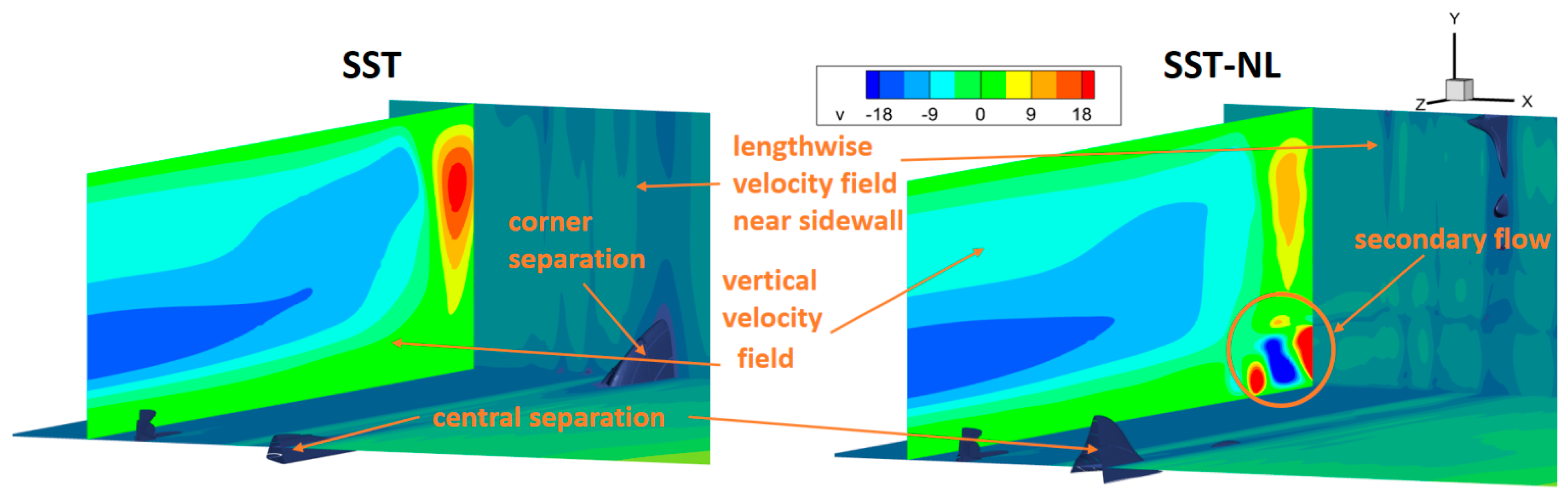
  • A significant influence on the pressure distribution along the duct and the shape of the separation zones is exerted by the nonlinear model of turbulent stresses in the case of the RANS approach and the generation of synthetic turbulence in the case of the IDDES approach.
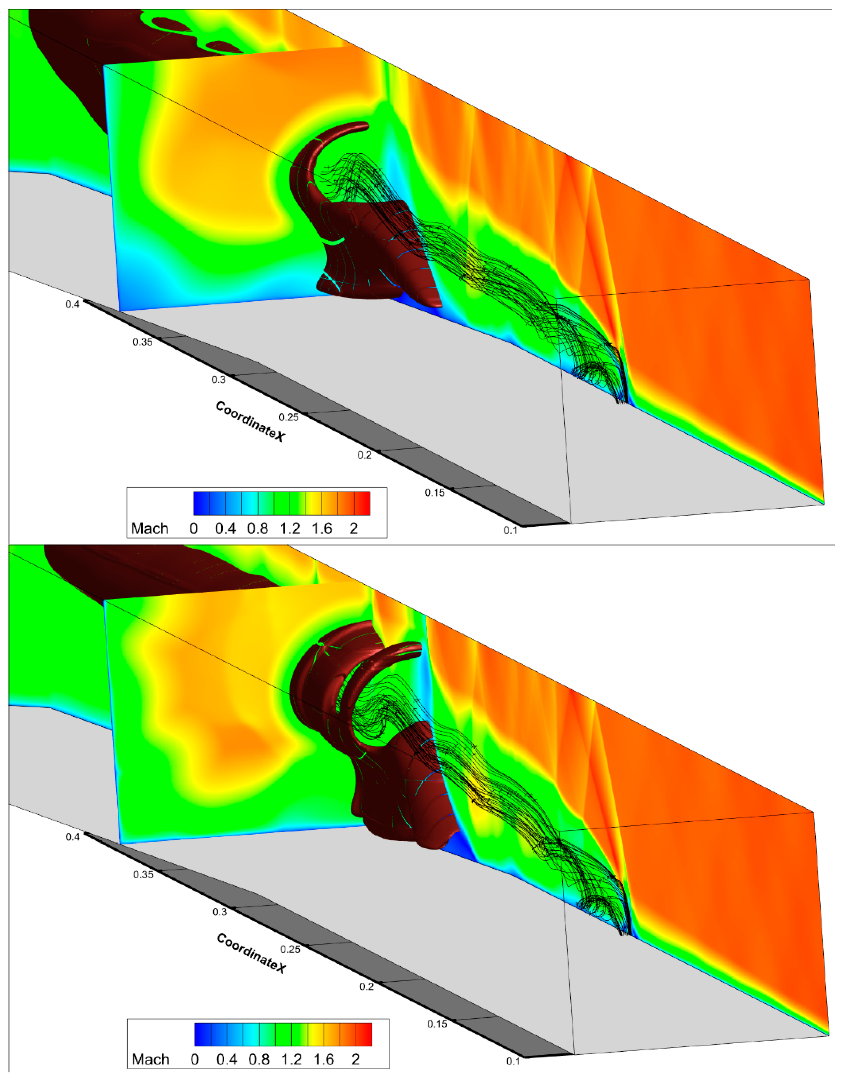
  • It was demonstrated that within the RANS framework, at a given wall temperature of 716 K, satisfactory agreement with the experimental pressure distribution can be achieved by increasing the roughness height from 65 to 85 μm if the secondary flows in the duct corners are reproduced in the simulation. In this case, the flow contains a large central separation and partial chocking, which does not contradict the Schlieren photographs taken in the experiment. However, no oscillations in this gas-dynamic structure were observed.
In the IDDES simulation, the central separation reached the injected jet and joined the recirculation region behind it. The streamwise pressure distribution in the region (0.3; 0.6) m along the X axis turns out to be significantly overestimated compared to the experiment and RANS simulations (Figure 10). This indicates a more intense heat release in this area. For comparison, Figure 17 shows the concentrations of OH radicals in the symmetry plane for the averaged IDDES simulation as well as RANS simulations with roughness heights of 65 and 80 μm. It can be seen that in the IDDES simulation, heat release begins sufficiently earlier in comparison with the RANS simulation. In the previous section, it was established that an increase in the eddy viscosity completely changes the flow pattern. All these facts indicate that in the eddy-resolving simulation, the conditions necessary for self-ignition (mixing of fuel and oxidizer, high temperatures and pressures) were formed much earlier.
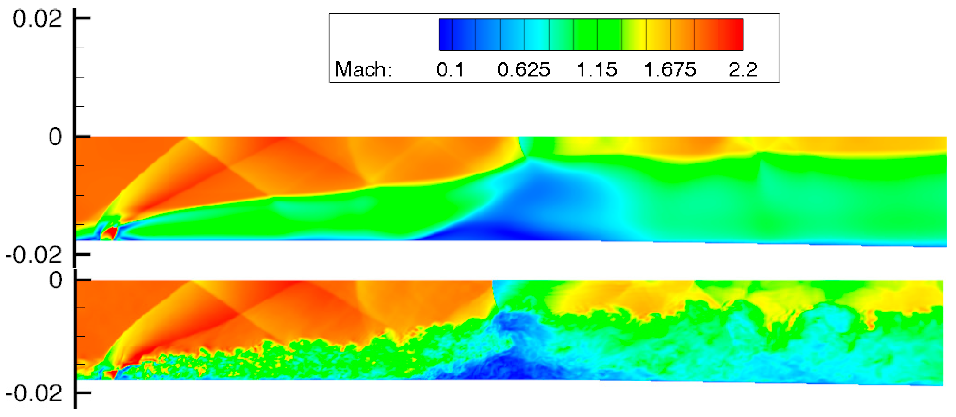
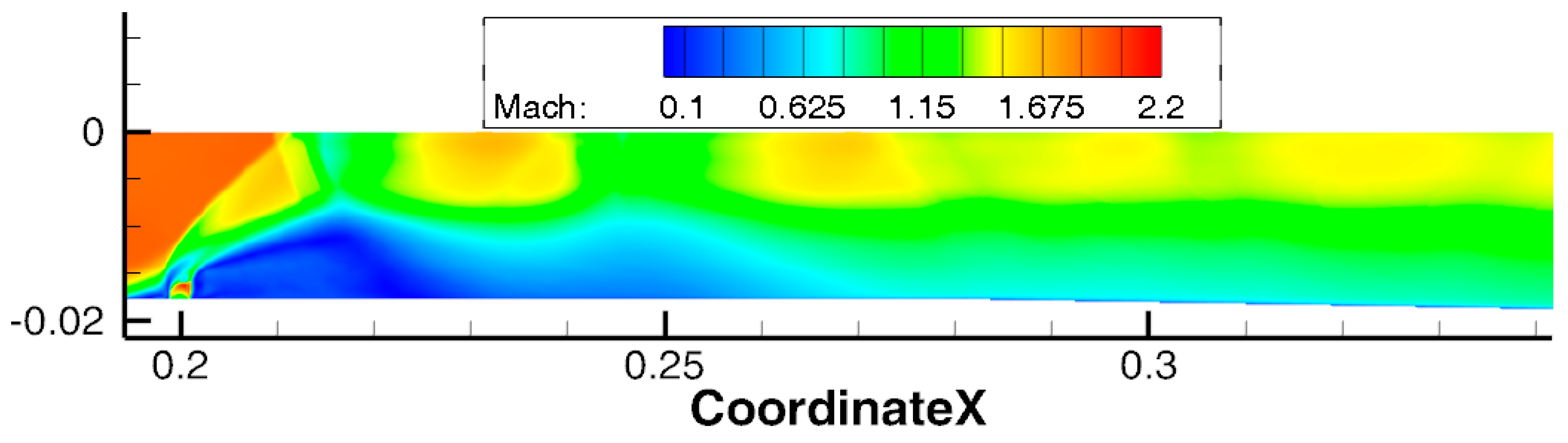
  • The first reason for excessive temperature and pressure values in the flow may be the initial field and the first 0.002 s of the simulation, during which hs = 80 μm was maintained. To check this, an IDDES simulation was run from the field obtained in the RANS simulation with hs = 65 μm. Figure 18 shows the simulation at the time moment 0.00204 s; the flow pattern is in good agreement with the experiment. However, the pressure distribution on the wall contains a second peak at x = 0.3 m, which is not present in the experiment. At the same time, the pressure is still overestimated in the area (0.3;0.6) m along the X axis (Figure 19). During further modeling, the gas-dynamic structure oscillated once along the X axis and reached the same state as the previous eddy-resolving simulation.
  • The second reason may be an incorrect description of the separation before the injection, as evidenced by the difference in the pressure distribution. In all simulations, the pressure level before injection is lower than in the experiment; see Figure 10 and Figure 19. In RANS simulations, this disadvantage is probably compensated by an increase in the roughness height. The question of modeling this separation using an eddy-resolving approach and its effect on the combustion process requires a separate study.
  • The third reason is a possibly excessive level of turbulence kinetic energy in the boundary layer upstream of the injection. The synthetic turbulence generator converts the turbulence energy received in RANS into resolved and subgrid energies while maintaining the total value. However, the initial value was obtained as a result of a relatively coarse simulation of the heater and may turn out to be too high. This may not affect RANS simulations but may be significant in eddy-resolving simulations. A decrease in the turbulence energy at the duct entrance will lead to a decrease in the subgrid energy. Therefore, the eddy viscosity and the quality of fuel mixed with oxidizer will decrease. This issue also needs to be researched separately.
  • The fourth reason is modeling only the lower half of the duct. According to experimental data kindly provided by Dr. A. Vincent-Randonnier, the selected mode is statistically symmetric (4098 snapshots were taken, and the correlation coefficient between the leading edges of the top and bottom flames ≈ 0.95). However, the instantaneous positions of the top and bottom flames can differ by up to 6 mm in the streamwise direction during the first 0.015 s of the simulation. In eddy-resolving simulations, this may turn out to be significant. This can be investigated by simulating the full model, which will require at least twice as many computational resources.

Author Contributions

Conceptualization, V.S. and V.V.; methodology, A.T. and A.S.; software, A.T., A.S. and S.B.; formal analysis, S.B.; research, S.B.; resources, V.V. and A.S.; data curation, S.B.; writing—original draft preparation, V.V. and S.B.; writing—review and editing, S.B., A.T., V.V., A.S. and V.S.; funding, A.S. All authors have read and agreed to the published version of the manuscript.

Funding

The research results related to the SST-NL model were obtained within Russian Science Foundation grant 22-29-00660, https://rscf.ru/project/22-29-00660/.

Data Availability Statement

The data presented in this study are available on request from the corresponding authors.

Acknowledgments

Many thanks to Axel Vincent-Randonnier and Guillaume Pelletier (ONERA) for multiple discussions of the results of experiments and simulations, as well as for providing additional information on the experimental conditions [22] and the simulations [24]. The authors are also grateful to Anna Budnikova, who helped with the translation of the text, and to Dmitry Afanasyev, who performed one-dimensional calculations.

Conflicts of Interest

The authors declare no conflict of interest.

References

  1. Zhiyin, Y. Large-eddy simulation: Past, present and the future. Chin. J. Aeronaut. 2015, 28, 11–24. [Google Scholar] [CrossRef]
  2. Piomelli, U. Large eddy simulations in 2030 and beyond. Philos. Trans. R. Soc. A 2014, 372, 2022. [Google Scholar] [CrossRef] [PubMed]
  3. Tkatchenko, I.; Kornev, N.; Jahnke, S.; Steffen, G.; Hassel, E. Performances of LES and RANS models for simulation of complex flows in a coaxial jet mixer. Flow Turbul. Combust. 2007, 78, 111–127. [Google Scholar] [CrossRef]
  4. Bogey, C.; Bailly, C. Computation of a high Reynolds number jet and its radiated noise using large eddy simulation based on explicit filtering. Comput. Fluids 2006, 35, 1344–1358. [Google Scholar] [CrossRef]
  5. Bres, G.A.; Lele, S.K. Modelling of jet noise: A perspective from large-eddy simulations. Philos. Trans. R. Soc. A 2019, 377, 2159. [Google Scholar] [CrossRef]
  6. Gaitonde, D.V. Progress in shock wave/boundary layer interactions. Prog. Aerosp. Sci. 2015, 72, 80–99. [Google Scholar] [CrossRef]
  7. Oefelein, J.C. Large eddy simulation of turbulent combustion processes in propulsion and power systems. Prog. Aerosp. Sci. 2006, 42, 2–37. [Google Scholar] [CrossRef]
  8. Spalart, P.R. Detached-eddy simulation. Annu. Rev. Fluid Mech. 2009, 41, 181–202. [Google Scholar] [CrossRef]
  9. Menter, F.; Hüppe, A.; Matyushenko, A.; Kolmogorov, D. An overview of hybrid RANS-LES models ddeveloped for industrial CFD. Appl. Sci. 2021, 11, 2459. [Google Scholar] [CrossRef]
  10. Oran, E.S.; Boris, J.P. Numerical Simulation of Reactive Flow, 2nd ed.; Cambridge University Press: Cambridge, UK, 2001; p. 540. Available online: https://citeseerx.ist.psu.edu/document?repid=rep1&type=pdf&doi=5e66cd1269fd730eb764ba71d60ddab94b558805 (accessed on 25 October 2023).
  11. Poinsot, T.; Veynante, D. Theoretical and Numerical Combustion; RT Edwards, Inc., 2005; p. 545. Available online: https://books.google.ru/books?hl=ru&lr=&id=cqFDkeVABYoC&oi=fnd&pg=PR11&dq=poinsot+combustion&ots=LftXMSQVex&sig=u42NxkhRjF_5LL8OPFDBgm-lv_s&redir_esc=y#v=onepage&q=poinsot%20combustion&f=false (accessed on 25 October 2023).
  12. Westbrook, C.K.; Mizobuchi, Y.; Poinsot, T.J.; Smith, P.J.; Warnatz, J. Computational combustion. Proc. Combust. Inst. 2005, 30, 125–157. [Google Scholar] [CrossRef]
  13. Poludnenko, A.Y.; Oran, E.S. The interaction of high-speed turbulence with flames: Global properties and internal flame structure. Combust. Flame 2010, 157, 995–1011. [Google Scholar] [CrossRef]
  14. Gatski, T.B. Second-moment and scalar flux representations in engineering and geophysical flows. Fluid Dyn. Res. 2009, 41, 12202. [Google Scholar] [CrossRef]
  15. Agostinelli, P.W.; Laera, D.; Boxx, I.; Gicquel, L.; Poinsot, T. Impact of wall heat transfer in Large Eddy Simulation of flame dynamics in a swirled combustion chamber. Combust. Flame 2021, 234, 111728. [Google Scholar] [CrossRef]
  16. Marusic, I.; McKeon, B.J.; Monkewitz, P.A.; Nagib, H.M.; Smits, A.J.; Sreenivasan, K.R. Wall-bounded turbulent flows at high Reynolds numbers: Recent advances and key issues. Phys. Fluids 2010, 22, 6. [Google Scholar] [CrossRef]
  17. Petranović, Z.; Edelbauer, W.; Vujanović, M.; Duić, N. Modelling of spray and combustion processes by using the Eulerian multiphase approach and detailed chemical kinetics. Fuel 2017, 191, 25–35. [Google Scholar] [CrossRef]
  18. Sun, X.; Liu, H.; Duan, X.; Guo, H.; Li, Y.; Qiao, J.; Liu, Q.; Liu, J. Effect of hydrogen enrichment on the flame propagation, emissions formation and energy balance of the natural gas spark ignition engine. Fuel 2022, 307, 121843. [Google Scholar] [CrossRef]
  19. Duan, X.; Xu, L.; Xu, L.; Jiang, P.; Gan, T.; Liu, H.; Ye, S.; Sun, Z. Performance analysis and comparison of the spark ignition engine fuelled with industrial by-product hydrogen and gasoline. J. Clean. Prod. 2023, 424, 138899. [Google Scholar] [CrossRef]
  20. Bakhne, S.; Troshin, A.; Sabelnikov, V.; Vlasenko, V. Improved delayed detached eddy simulation of combustion of hydrogen jets in a high-speed confined hot air cross flow. Energies 2023, 16, 1736. [Google Scholar] [CrossRef]
  21. Vincent-Randonnier, A.; Moule, Y.; Ferrier, M. Combustion of hydrogen in hot air flows within LAPCAT-II dual mode ramjet combustor at Onera-LAERTE facility-Experimental and numerical investigation. AIAA Pap. 2014, 2014–2932. [Google Scholar] [CrossRef]
  22. Balland, S.; Vincent-Randonnier, A. Numerical study of hydrogen/air combustion with CEDRE code on LAERTE dual mode ramjet combustion experiment. AIAA 2015, 2015–3629. [Google Scholar] [CrossRef]
  23. Vincent-Randonnier, A.; Sabelnikov, V.; Ristori, A.; Zettervall, N.; Fureby, C. An experimental and computational study of hydrogen–air combustion in the LAPCAT II supersonic combustor. Proc. Comb. Inst. 2019, 37, 3703–3711. [Google Scholar] [CrossRef]
  24. Pelletier, G.; Ferrier, M.; Vincent-Randonnier, A.; Sabelnikov, V.; Mura, A. Wall roughness effects on combustion development in confined supersonic flow. J. Propuls. Power 2021, 37, 151–166. [Google Scholar] [CrossRef]
  25. Sabelnikov, V.A.; Troshin, A.I.; Bakhne, S.; Molev, S.S.; Vlasenko, V.V. Poisk opredeljajushhih fizicheskih faktorov v validacionnyh raschetah jeksperimental’noj modeli ONERA LAPCAT II s uchetom sherohovatosti stenok kanala. (Search for determining physical factors in variational simulations of the experimental model ONERA LAPCAT II, taking into account the roughness of the duct walls.). Goren. I Vzryv (Combust. Explos.) 2021, 14, 55–67. (In Russian) [Google Scholar] [CrossRef]
  26. Reynolds, O. On the dynamical theory of incompressible viscous fluids and the determination of the criterion. Proc. R. Soc. Lond. 1894, 56, 40–45. [Google Scholar]
  27. Bruce, P.J.K.; Burton, D.M.F.; Titchener, N.A.; Babinsky, H. Corner effect and separation in transonic channel flows. J. Fluid Mech. 1997, 679, 247–262. [Google Scholar] [CrossRef]
  28. Bruce, P.J.K.; Babinsky, H.; Tartinville, B.; Hirsch, C. Corner effect and asymmetry in transonic channel flows. AIAA J. 2011, 49, 2382–2392. [Google Scholar] [CrossRef]
  29. Boychev, K. Shock Wave-Boundary-Layer Interactions in High-Speed Intakes. Ph.D. Thesis, University of Glasgow, Glasgow, Scotland, 2021. Available online: https://theses.gla.ac.uk/82577/ (accessed on 8 February 2023).
  30. Sabnis, K. Supersonic Corner Flows in Rectangular Ducts. Ph.D. Thesis, University of Cambridge, Cambridge, UK, 2020. [Google Scholar] [CrossRef]
  31. Spalart, P.R. Strategies for turbulence modeling and simulations. Int. J. Heat Fluid Flow 2000, 21, 252–263. [Google Scholar] [CrossRef]
  32. Mani, M.; Babcock, D.; Winkler, C.; Spalart, P.R. Predictions of a supersonic turbulent flow in a square duct. In Proceedings of the 51st AIAA Aerospace Sciences Meeting, Dallas, TX, USA, 7–10 January 2013. [Google Scholar] [CrossRef]
  33. Shur, M.L.; Spalart, P.R.; Strelets, M.K.; Travin, A.K. Synthetic Turbulence Generators for RANS-LES Interfaces in Zonal Simulations of Aerodynamic and Aeroacoustic Problems. Flow Turbul. Combust 2014, 93, 63–92. [Google Scholar] [CrossRef]
  34. Liu, W. Analysis of factors determining numerical solution in the calculation of flow with combustion using the ONERA experimental model. Thermophys. Aeromech. 2023, 30, 507–523. [Google Scholar] [CrossRef]
  35. Fureby, C. Large eddy simulations of the LAPCAT-II and the SSFE combustor configurations. AIAA SciTech Forum 2020, 2020-1109. [Google Scholar] [CrossRef]
  36. Volino, R.J.; Devenport, W.J.; Piomelli, U. Questions on the effects of roughness and its analysis in non-equilibrium flows. J. Turb. 2022, 23, 454–466. [Google Scholar] [CrossRef]
  37. Aupoix, B. Roughness corrections for the k-w SST model: Status and proposals. J. Fluids Eng. 2015, 137, 21202. [Google Scholar] [CrossRef]
  38. Latin, R.M.; Bowersox, R.D. Flow Properties of a Supersonic Turbulent Boundary Layer with Wall Roughness. AIAA J. 2000, 38, 10. [Google Scholar] [CrossRef]
  39. Schlichting, H. Experimental Investigation of the Problem of Surface Roughness; Technical Memorandums National Advisory Committee for Aeronautics: Washington, DC, USA, 1937. [Google Scholar]
  40. Troshin, A.I.; Molev, S.S.; Vlasenko, V.V.; Mikhailov, S.V.; Bakhne, S.; Matyash, S.V. Modelirovanie turbulentnih tecenii na osnove podhoda IDDES s pomosciu programmi zFlare (Simulation of turbulent flows based on the IDDES approach using the zFlare solver). Vici. Meh. Splosh. sred (Comput. Contin. Mech.) 2023, 16, 203–218. [Google Scholar] [CrossRef]
  41. Bosnyakov, S.; Kursakov, I.; Lysenkov, A.; Matyash, S.; Mikhailov, S.; Vlasenko, V.; Quest, J. Computational tools for supporting the testing of civil aircraft configurations in wind tunnels. Progr. Aerosp. Sci. 2008, 44, 67–120. [Google Scholar] [CrossRef]
  42. Menter, F.R.; Kuntz, M.; Langtry, R. Ten years of industrial experience with the SST turbulence model. Turbul. Heat Mass Transf. 2003, 4, 625–632. Available online: https://cfd.spbstu.ru/agarbaruk/doc/2003_Menter,%20Kuntz,%20Langtry_Ten%20years%20of%20industrial%20experience%20with%20the%20SST%20turbulence%20model.pdf (accessed on 8 February 2023).
  43. Suga, K.; Craft, T.J.; Iacovides, H. An analytical wall-function for turbulent flows and heat transfer over rough walls. Int. J. Heat Fluid Flow 2006, 27, 852–866. [Google Scholar] [CrossRef]
  44. Zhang, R.; Zhang, M.; Shu, C.W. On the order of accuracy and numerical performance of two classes of finite volume WENO schemes. Commun. Comput. Phys. 2011, 9, 807–827. [Google Scholar] [CrossRef]
  45. Suresh, A.; Huynh, H. Accurate Monotonicity-Preserving Schemes with Runge–Kutta Time Stepping. J. Comput. Phys. 1997, 136, 83–99. [Google Scholar] [CrossRef]
  46. Gritskevich, M.S.; Garbaruk, A.V.; Schütze, J.; Menter, F.R. Development of DDES and IDDES formulations for the k-ω Shear Stress Transport model. Flow Turb. Comb. 2011, 88, 431–449. [Google Scholar] [CrossRef]
  47. Guseva, E.K.; Garbaruk, A.V.; Strelets, M.K. An automatic hybrid numerical scheme for global RANS-LES approaches. J. Phys. IOP Pub. Conf. Ser. 2017, 929, 12099. [Google Scholar] [CrossRef]
  48. Bakhne, S.; Sabelnikov, V.A. Method for choosing the spatial and temporal approximations for the LES approach. Fluids 2022, 7, 376. [Google Scholar] [CrossRef]
  49. Bakhne, S.; Troshin, A.I. Comparison of upwind and symmetric WENO schemes in large eddy simulation of basic turbulent flows. Comput. Math. Math. Phys. 2023, 63, 1122–1136. [Google Scholar] [CrossRef]
  50. Jachimowski, C.J. An Analysis of Combustion Studies in Shock Expansion Tunnels and Reflected Shock Tunnels; Technical Paper 3224; NASA: Hampton, VA, USA, 1992.
  51. Matyushenko, A.A.; Garbaruk, A.V. Non-linear correction for the k-ω SST turbulence model. J. Phys. IOP Pub. Conf. Ser. 2017, 929, 12102. [Google Scholar] [CrossRef]
  52. Menter, F.R.; Garbaruk, A.V.; Egorov, Y. Explicit algebraic Reynolds stress models for anisotropic wall-bounded flows. Prog. Flight Phys. 2012, 3, 89–104. [Google Scholar] [CrossRef]
  53. Raiesi, H.; Piomelli, U.; Pollard, A. Evaluation of Turbulence Models Using Direct Numerical and Large-Eddy Simulation Data. J. Fluids Eng. 2011, 133, 021203. [Google Scholar] [CrossRef]
  54. Savelyev, A.A.; Kursakov, I.A.; Matyash, E.S.; Streltsov, E.V.; Shtin, R.A. Application of the Nonlinear SST Turbulence Model for Simulation of Anisotropic Flows. Supercomput. Front. Innov. 2022, 9, 38–48. [Google Scholar] [CrossRef]
  55. Pelletier, G.; Ferrier, M.; Vincent-Randonnier, A.; Mura, A. Delayed Detached Eddy Simulations of Rough-Wall Turbulent Reactive Flows in a Supersonic Combustor. In Proceedings of the 23rd AIAA International Space Planes and Hypersonic Systems and Technologies Conference, Montreal, QC, Canada, 10–12 March 2020. [Google Scholar] [CrossRef]
  56. Mikheev, M.A. Rasciotnie formuli konvektivnogo teploobmena (Calculation formulas for convective heat transfer). Izv. AN SSSR (Izv. USSR Acad. Sci.) 1966, 5, 96–105. [Google Scholar]
  57. Abramovich, G.N. Applied Gas Dynamics, 3rd ed.; Defense Technical Information Center: Fort Belvoir, VA, USA, 1973; p. 1139.
  58. Garbaruk, A. Eddy-Resolving Methods. Turbulence Modeling. 2019. Available online: https://cfd.spbstu.ru/agarbaruk/SRS_methods/Term10_Part2_Lec02_les_chan.pdf (accessed on 8 August 2023).
  59. Troshin, A.; Bakhne, S.; Sabelnikov, V. Numerical and Physical Aspects of Large-Eddy Simulation of Turbulent Mixing in a Helium-Air Supersonic Co-Flowing Jet. In Progress in Turbulence IX; Örlü, R., Talamelli, A., Peinke, J., Oberlack, M., Eds.; Springer: Berlin/Heidelberg, Germany, 2021; pp. 297–302. [Google Scholar] [CrossRef]
Figure 1. The sketch of the ONERA LAERTE experimental set-up. The figure was courteously provided by Dr. A. Vincent-Randonnier.
Energies 16 07262 g001
Figure 2. Profiles of the streamwise and spanwise velocity at the diagonal of the duct cross section (DNS [53], SST-NL [51], zFlare).
Energies 16 07262 g002
Figure 3. Computational domain. Block boundaries are shown. C1—compartment of constant cross-section; C2, C4—compartments with expansion 2°; C3—compartment with expansion 6°; C5—expanding buffer block with slip walls.
Energies 16 07262 g003
Figure 4. Grid near the hydrogen injection.
Energies 16 07262 g004
Figure 5. Temperature distributions at different times.
Energies 16 07262 g005
Figure 6. Mach number in the symmetry plane, RANS simulations. The simulation with the initial boundary condition is shown in the top image, and the bottom image presents the results with the windows taken into account.
Energies 16 07262 g006
Figure 7. Structure of separations (flow is directed from left to right). RANS simulation using the SST (left) and SST-NL (right) models.
Energies 16 07262 g007
Figure 8. Influence of secondary flows (flow is directed from left to right). RANS simulation using the SST (top) and SST-NL (bottom) models. A quarter of the duct is shown.
Energies 16 07262 g008
Figure 9. Radical OH concentration isosurface = 0.017 (flow is directed from right to left). RANS simulation using the SST (top) and SST-NL (bottom) models. A quarter of the duct is shown.
Energies 16 07262 g009
Figure 10. Pressure distribution along the duct: RANS simulations with the SST model and hs = 65 µm (blue line), with the SST-NL model and hs = 65 µm (pink line), 80 µm (orange line), 85 µm (green line), 90 µm (turquoise line); IDDES simulations with hs = 65 µm at the times 2.88 ms (red line) and 4.88 ms (brown line) and the experimental data (black dots) [21] are also shown.
Energies 16 07262 g010
Figure 11. Mach number field in the symmetry plane. RANS simulations with hs = 65, 80, and 90 µm (from top to bottom).
Energies 16 07262 g011
Figure 12. Temperature field in the symmetry plane. RANS simulations with hs = 80 and 90 µm (from top to bottom).
Energies 16 07262 g012
Figure 13. Mach number field in the symmetry plane in the vicinity of the injection. The IDDES without an STG from [20] (top) and the IDDES with an STG (bottom).
Energies 16 07262 g013
Figure 14. Mach number field in the symmetry plane. RANS simulation (top image) and the IDDES simulation (from top to bottom, at consecutive moments in time) are presented.
Energies 16 07262 g014aEnergies 16 07262 g014b
Figure 15. Averaged Mach number field in the symmetry plane in the IDDES simulation.
Energies 16 07262 g015
Figure 16. Instantaneous Mach number field in the symmetry plane in the IDDES simulation with an increased subgrid viscosity.
Energies 16 07262 g016
Figure 17. Concentration field of OH radicals in the symmetry plane. (a) averaged IDDES simulation, (b) RANS simulation with hs = 65 µm, (c) RANS simulation with hs = 80 µm.
Energies 16 07262 g017
Figure 18. Fields of OH radicals concentration and Mach number in the plane of symmetry at the time instant 0.00204 s. IDDES simulation from the initial RANS field with hs = 65 µm.
Energies 16 07262 g018
Figure 19. Instantaneous streamwise pressure distribution on the wall at time 0.00204 s. IDDES simulation from the initial RANS field with hs = 65 µm.
Energies 16 07262 g019
Disclaimer/Publisher’s Note: The statements, opinions and data contained in all publications are solely those of the individual author(s) and contributor(s) and not of MDPI and/or the editor(s). MDPI and/or the editor(s) disclaim responsibility for any injury to people or property resulting from any ideas, methods, instructions or products referred to in the content.

