Optimising Highway Energy Harvesting: A Numerical Simulation Study on Factors Influencing the Performance of Vertical-Axis Wind Turbines

Abstract

Vertical-axis wind turbines (VAWTs) are an innovative solution for energy harvesting, as they harness the power of the wind by enabling rotational motion around a vertical shaft situated on the ground. This paper deals with the design optimisation of VAWT systems for highway energy harvesting. The four design parameters, blade number, blade curvature angle, blade thickness and blade diameter ratio, have been investigated to find their respective optimalities for the enhanced energy efficiency of VAWT systems. Computational fluid dynamics (CFD) simulations are conducted in Ansys Fluent using a Banki turbine model created in Solidworks^®, with a constant velocity inlet of 4 m/s and rotational speeds ranging from 0.5 to 3 rad/s. The simulations consider the placement of the turbine in the central reservation of a highway with a windshield for enhanced performance. From the results, it was observed that increasing blade thickness and blade number improve turbine performance, with maximum power coefficients achieved at specific tip speed ratios (TSRs). The optimal blade diameter ratio has been found to be approximately 0.75 for TSR values between 0.1 and 0.5, whilst a ratio of 0.83 gave the best performance at higher TSR values. Also, a blade curvature angle of 60 degrees has been found optimal for slow rotations, while 100 degrees yielded the highest power coefficient for faster rotations. The study could also highlight the significance of blade curvature angle variation, resulting in a notable 14% performance increase compared to the baseline. The geometric changes proposed in the study allow for greater power extraction from the same turbine footprint, leading to increased energy efficiency in VAWT systems.

1. Introduction

Alternative and innovative methods of renewable energy harvesting are constantly being researched and developed as divergence away from our reliance on fossil fuels is accelerated [1]. This paper explores a relatively uncharted means of energy harvesting in the form of Vertical-Axis Wind Turbines (VAWTs) designed for use in the central reservation of a highway in which they capture the wake energy of passing vehicles from both sides. The paper intends to explore an alternative solution to renewable energy generation which is of utmost importance in the current climate crisis. On identifying the need for utilisation of vast untapped energy from the air wake of vehicles, this paper attempts to explore the VAWT performance factors that would increase the efficiency and therefore viability of this energy-harvesting method. Similar studies demonstrate the viability of power generation [2,3] from the usable and substantial value of power obtained, meaning capturing this energy would be highly useful in the drive to a sustainable future by making use of every available resource.

VAWTs are a type of wind turbine where the rotational motion occurs vertically to the ground. They are typically much smaller than the more common Horizontal-Axis Wind Turbine (HAWT) used extensively today [4] and there exist two main VAWT types. Darrieus wind turbines utilise the lift principle from air flowing over the aerofoil, generating lift, and are commonly seen in helical geometries [5]. A Savonius wind turbine is a drag type, which features blades and/or scoops that catch air flow to spin the turbine [5]. Within these two types are sub-categories of VAWTs which have many different geometric designs that suit different operating conditions, such as the drag-type Banki turbine which is studied in the current paper. The Banki or cross-flow turbine has prominent use in hydro-power applications and design processes [6,7,8] where water drives the turbine to generate electricity. The flow performance characteristics are very similar in either medium (air or water). However, due to water’s much greater density it is likely that forces acting on turbine blades are greater with water. Study [6] obtains CFD cross-flow contours depicting water flow characteristics. The study concludes that the turbine has low efficiency at 50 RPM and proceeds to find an optimal RPM of 125 to negate the effects of so-called recirculation phenomena in which water interacts negatively with the runner shaft. The studies [7,8] attempt to create effective equations in dimensionless form to select the optimal number of blades for particular TSR values, rotational speeds, runner material and blade thickness. It is unclear whether these can be transferred to an air-based medium application.

VAWTs were used in their primitive form as early as the 7th century in the Middle East and possess several advantages over the HAWT [9]. They have the ability to function omni-directionally, meaning they can be installed anywhere and do not require a yaw system to stay in the direction of the prevailing wind. This, along with their smaller form factor, means a greater ease of installation and maintenance as complex parts are found at the base. It is considered that for installations up to 10 kW, VAWTs emit less noise than HAWTs, which is particularly important for urban areas as this is the ideal installation place due to the turbulent flows of the environment created by passing vehicles [10]. Despite these advantages, VAWTs face certain drawbacks that hinder their practical implementation for energy-harvesting purposes. One such limitation is that they are prone to oscillations in torque, whereas the blades of a HAWT exert a constant torque [11]. This is because each blade has a different angle of attack as a function of time and therefore experiences a different force which produces varying torque. Therefore, wear is a big issue as it can become uneven. Hence, VAWTs that have a greater number of blades tend to suffer less from this issue as the force applied is distributed more evenly, although this increases the mass and therefore rotational inertia of the system which inhibits power generation. Another drawback is that they are less efficient than HAWTs [12]; however, this can be combated by their small form factor and therefore can be situated with a greater density. Owing to these disadvantages, the implementation of VAWTs for highway energy harvesting has been limited in experimental and commercial applications. However, academic research in this field has been increasing over the past 5–10 years as researchers explore new energy-harvesting solutions [13,14]. Commercial examples, such as the ‘Alpha 311’ start-up company, demonstrate ongoing efforts to incorporate VAWTs into existing infrastructure, such as lamp posts in highway central reservations in the UK [15]. Prior academic studies explored different geometric designs [16], the blade thickness [17], the diameter ratio [18] and the effect of blade number on drag-type VAWT performance [19]. The findings from these studies have influenced the design parameters explored in the present study, encompassing blade thickness, diameter ratio, blade number and curvature angle. Notably, the novelty of this study provides an optimum blade-angle curvature of a VAWT which is not achieved in [20] due to the small-angle geometry set from 0 to 60 degrees. Other than this example, to the best of the authors’ knowledge, the specific geometry variation of blade-angle curvature cannot be found in the related academic literature. The study extends previous work [17,18,19] by considering a wider range of blade number configurations, equidistant blade thicknesses and a greater variation of inner diameter ratio.

This paper aims to assess how different geometric variations will affect the performance of a Banki wind turbine with the overarching quest of finding the highest-performing geometry and the most crucial geometric change in terms of the coefficient of power. Empirically, the higher the coefficient of power achieved by a given design, the more efficient it will be at capturing incoming air wakes, thus producing more energy. Initially, an attempt is made to identify the most suitable type of VAWT to use for the highway energy-harvesting application. Once chosen, each geometry set (blade number, blade curvature angle, blade thickness and blade diameter ratio) is created in Solidworks^® [21] as a parasolid model. Each model is based on a Banki wind turbine design and is used in the simulations with Ansys Fluent. The Banki turbine is chosen as it exhibits the best performance in terms of power generated from the wake of a moving vehicle out of all VAWT types for the flow conditions created by vehicle wakes [22]. The computational geometry domain, mesh and setup are created for each design in Ansys Workbench [23].

In this study, the simulations are conducted at a speed of 4 m/s, which mimics the conditions experienced by a VAWT placed in the central reservation of a highway [24]. Notably, results of a previous study show [25] that whilst straight-bladed turbines exhibited poor performance, a curved design versus a twisted Savonius design yields no difference in performance. Thus, for simplicity, the curved design is adopted for all the designs. A baseline geometry on which all the designs are based is initially established. Each geometry variation has five designs, with two equidistant above and below the baseline (0.67 diameter ratio, 10 mm thickness, 80 degrees curvature and 20 blades). Subsequently, each parasolid model and their respective setup in Ansys Workbench is created. At the end of a simulation, extraction of performance data files allows the computation of the performance parameters: average power and torque coefficients, average torque value and peak average power output. From this, the effect of each geometry has been analysed, and suggestions on the optimal design are made.

The major contributions of this study include the design of multiple VAWT models in Solidworks^® and the identification of the most suitable model through the literature for analysing the highway energy-harvesting application. The paper also features the optimisation of four critical design parameters, blade number, blade curvature angle, blade thickness and blade diameter ratio, for maximum energy efficiency operation of VAWT systems.

2. Model Equations for CFD Analysis

Ansys Fluent is based on the finite volume method approach. This approach divides the flow region into small control volumes (cells) which make up the overall mesh of a geometry. The flow in and out of each cell is expressed by the integral form of the conservation equations with respect to the volume of each cell, whereby a set of linear algebraic equations can be obtained and solved [26]. The Navier–Stokes equations govern the physical properties of fluids for mass, momentum and energy. In this specific 2D case, only two equations for the incompressible Navier–Stokes are present, representing the x and y components with the addition of the continuity equation which is given by

$$\frac{\partial \rho }{\partial t}+\frac{\partial u}{\partial x}+\frac{\partial v}{\partial y}=0,$$

(1)

where each term represents conservation of mass in their respective direction and u and v are velocity components.

The Navier–Stokes equation representing X-axis momentum (Horizontal) is given by

$$\frac{\partial u}{\partial t}+u\frac{\partial u}{\partial x}+v\frac{\partial u}{\partial y}=-\frac{1}{\rho }\frac{\partial \rho }{\partial x}+v\left(\frac{{\partial }^{2}u}{\partial x^2}+\frac{{\partial }^{2}u}{\partial y^2}\right),$$

(2)

where t is time and $\rho$ is density.

The Navier–Stokes equation representing Y-axis momentum (vertical) is given by

$$\frac{\partial v}{\partial t}+u\frac{\partial v}{\partial x}+v\frac{\partial v}{\partial y}=-\frac{1}{\rho }\frac{\partial \rho }{\partial y}+v\left(\frac{{\partial }^{2}v}{\partial x^2}+\frac{{\partial }^{2}v}{\partial y^2}\right).$$

(3)

The k-$\omega$ shear stress transport (SST) turbulence model is used in these simulations to model the turbulence terms in the Reynolds-averaged Navier–Stokes (RANS) equations. The model is merited for its ability in flow separation, which is likely to occur with rotating blades and exhibits good operation in adverse pressure gradients [27]. This model has been used successfully in similar applications with rotating VAWTs [2,3] which proves its suitability for the case.

The equations for the k-w SST model are a two-equation eddy-viscosity model [28]. The ‘k’ part or the turbulent kinetic energy determines the energy in the turbulence and is given by:

$$\frac{\partial k}{\partial t}+U_j\frac{\partial k}{\partial x_j}=P_k-\beta ·k\omega +\frac{\partial }{\partial x_j}\left[\left(\nu +{\sigma }_k{\nu }_T\right)\frac{\partial k}{\partial x_j}\right]$$

(4)

The ‘w’ or specific dissipation rate determines the rate of dissipation per unit turbulent kinetic energy and is given by:

$$\frac{\partial \omega }{\partial t}+U_j\frac{\partial \omega }{\partial x_j}=\alpha S^2-\beta {\omega }^2+\frac{\partial }{\partial x_j}\left[\left(\nu +{\sigma }_{\omega }{\nu }_T\right)\frac{\partial \omega }{\partial x_j}\right]+2(1-F_1){\sigma }_{\omega 2}\frac{1}{\omega }\frac{\partial k}{\partial x_i}\frac{\partial \omega }{\partial x_i}$$

(5)

Performance of a VAWT can be characterised by the torque coefficient:

$$C_m=\frac{M_a}{0.5\rho v_{\infty }^2{D}_{2}A}$$

(6)

and the power coefficient:

$$C_P=\frac{P_a}{0.5\rho v_{\infty }^{3}A}=TSR·C_m$$

(7)

where $M_a$ is the average moment acting on the turbine, $P_a$ is the average power acting on the turbine, $v_{\infty }$ is the free-stream velocity, $R_1$ is the radius and A is the area of the turbine.

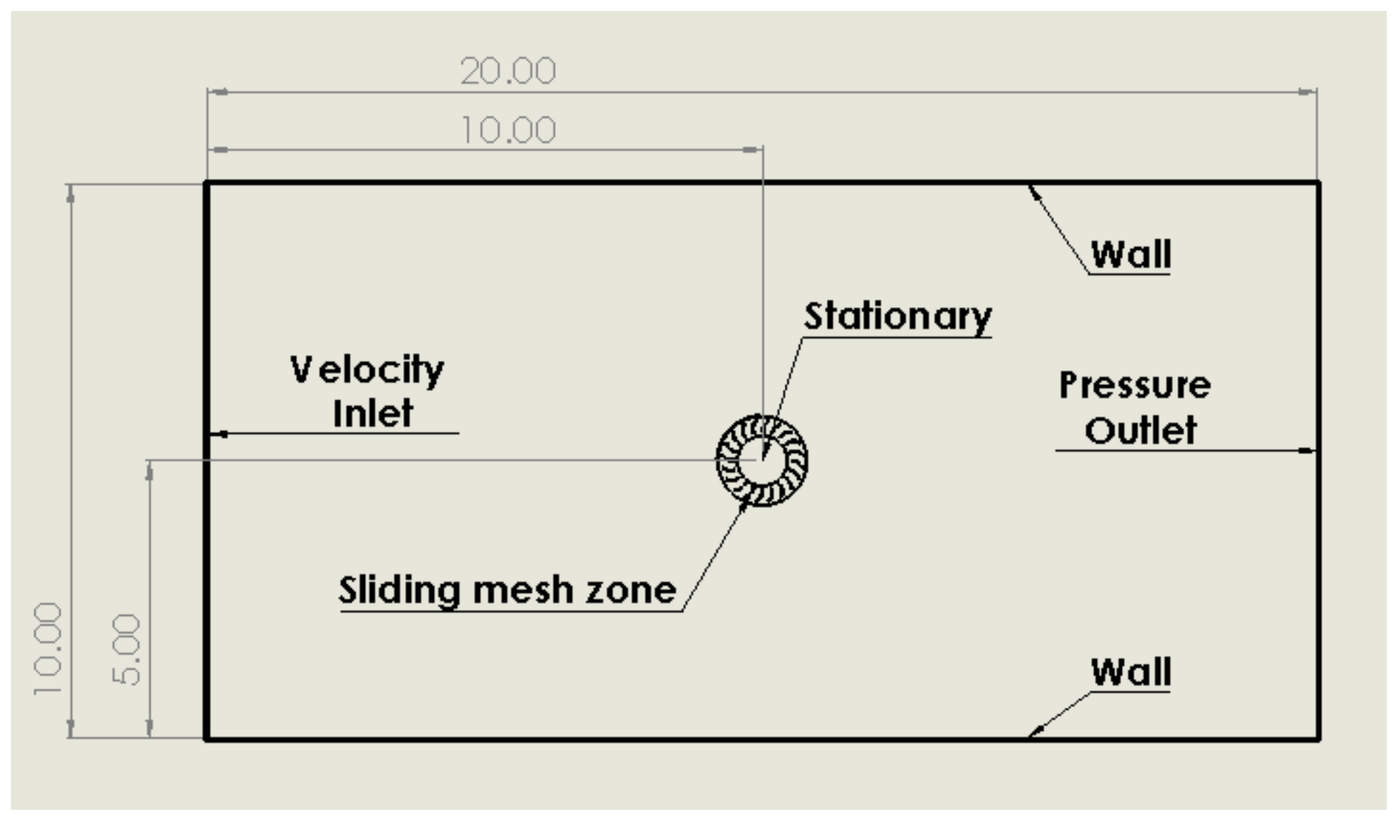
2.1. Setup and Modelling Method

For VAWT CFD simulations, there are two modelling methods that may be considered: moving reference frame (MRF) or sliding mesh method. However, it is inaccurate to model with the MRF approach because the wind turbine blade location versus the wind direction will change with time. Consequently, the sliding mesh approach is adopted, which is a moving mesh. This means that the geometry of the blades moves with it. The sliding mesh is the most accurate method, although more computationally expensive than the MRF approach [29]. The moving mesh is specified in the initial cell zone conditions for the inner rotating VAWT zone. The movement relative to the cell zone is set to ‘absolute’ within the CFD software for each rotational speed from 0.5 to 3 rad/s with revolution about the turbine axis origin (0,0). The interfaces between the computational domain and the inner VAWT zone were specified as an interface to allow for the transport of flow properties. Within each simulation, 400 timesteps at 20 iterations per timestep were adopted. To avoid large movements per timestep resulting in errors, 3 degrees rotation per timestep was adopted with the aim of the same number of revolutions per simulation period of 3. This choice can be justified through successful use in a similar study [2] where 1 degree per timestep was used; however, this involved high velocities up to around 40 m/s and therefore higher velocity gradients. Hence, a larger timestep by a factor of 3 was considered to be adequate when velocities did not exceed 10 m/s in this study. To achieve this at different rotational speeds, the timestep size was altered from 0.1 s for 0.5 rad/s to 0.017 s for 3 rad/s. Whilst this changed the flow time that was simulated, the number of rotations and iterations for each rotational speed and geometry were kept the same. In all simulations, the residual convergence criteria of 10⁻⁵ were specified.

2.2. Initial Conditions and Model Assumptions

Within each simulation, the density of inlet air was set to 1.225 kg/m³ with the dynamic viscosity at $1.7894\times {10}^{-5}$ Ns/m² and the pressure outlet was set to the standard atmospheric value of 101,325 Pa. These values were chosen to recreate conditions that a VAWT would likely experience in the UK (at sea level and 15 degrees Celsius). The air was set to incompressible to simplify the study and would likely not make any difference versus compressible flow due to the low velocity of inlet air.The baseline turbine geometry had an inner blade tip diameter of 1 m which extended outwards to 1.5 m. The computational domain in Figure 1 is such that the length is 13+ times the turbine diameter and the width is 6+ times the diameter. This particular size was chosen to negate errors caused by the influence of walls and was considered adequate when compared to similar studies [3,19,24,26,29,30].

An assumption within the simulations is the inlet velocity speed from the previously mentioned finding of the average air wake speed from passing vehicles at 4.4 m/s [24]. This value is obviously subject to change with factors such as vehicle type and shape, vehicle speed, distance away in the x-direction and the height at which this value was obtained. Thus, for ease of calculations, 4 m/s inlet velocity was used for all subsequent simulations. With this chosen inlet speed, the Reynold’s number for all simulations was ≈400,000.

3. Simulation Work and Designs

3.1. Initial Design Geometries

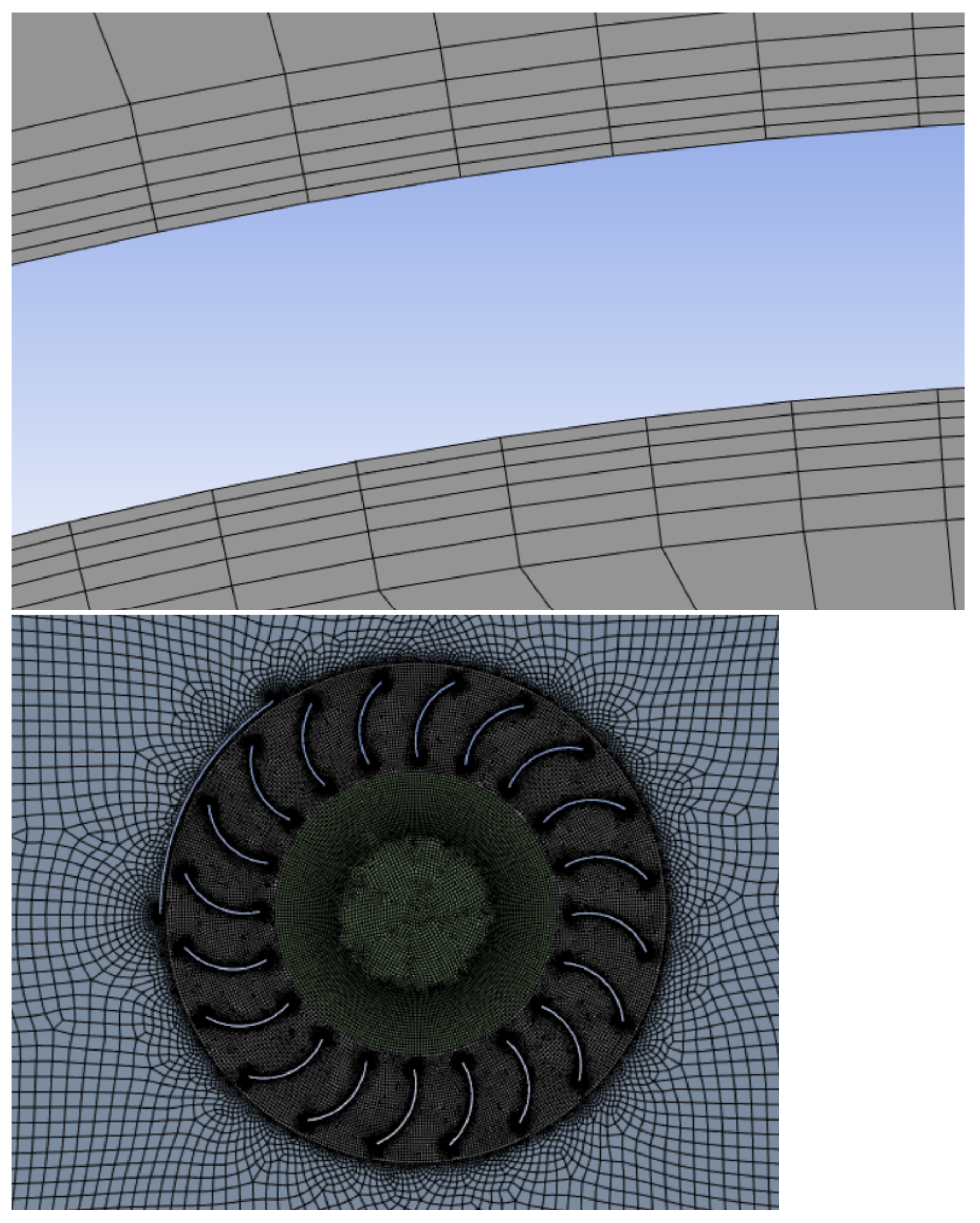
The initial design takes inspiration from a previous study [3] and is denoted as the ‘baseline’ which each geometry variation varies from. This is a 20-bladed Banki turbine design at 10 mm thickness, 0.67 blade diameter ratio and 80 degrees curvature with blade tips at tangent to an inner radius of 1 m and outer radius of 1.5 m situated in a rotating domain of 1.6 m as shown in Figure 2 (left), with the addition of a windshield [30,31], where 60 degrees of the circle is ‘shielded’ against incoming air for all designs as shown in Figure 2 (right). This addition of the windshield prevents negative torque acting against the turbine which occurs on the convex side of a blade, with 60 degrees being the angle most effective out of a range of 0 (no windshield) to 150 degrees, varied in 30-degree increments.

From this, the number of blades was varied to find the effect of blade number variation on performance. A set of five different blade number turbines were created, with equal differencing of blade number about the baseline of 20. Thus, this resulted in turbine blade configurations of 16, 18, 20, 22 and 24. Each required its own geometry and meshing setup in Ansys workbench for use in Ansys Fluent.

The blade curvature angles were varied by adopting the same method with 0 degrees being a straight line and 180 degrees as the shape of a semicircle. The initial model had 80 degrees curvature and the subsequent four further variations were 40, 60, 100 and 120 degrees. The same procedure was followed for blade thickness with the baseline at 10 mm blade thickness. In increments of 2.5 mm, blade thickness increased from 5 mm to 15 mm. The blade diameter ratio was varied between 0.83 and 0.5 where 0.5 has blades with the longest chord length. To keep the outer edge position of each blade and the sliding mesh area the same, the inner diameter (D1) was varied from 0.75 m to 1.25 m, whilst keeping the outer diameter (D2) the same. The baseline diameter ratio was 0.75 and corresponds to a 1 m inner diameter. Figure 3 presents the geometrical parameters explored in this paper as explained. The diameter ratio is given by the ratio of D1/D2, where D1 is the inner diameter between opposite blade tips and D2 is the outer diameter of the outer blade tips.

3.2. Model Mesh

Ansys workbench formed the backbone of each geometry setup and meshing. Initially, a parasolid model created in Solidworks^® was imported and the computational domain was sketched and constructed around this in Ansys DesignModeler for which several Boolean operations were performed to separate surface bodies and the blade walls. Once complete, the mesh was created the same on each design using Ansys meshing. This meant that each model had a similar element number of ≈150,000 elements and an equally fine mesh in areas of high gradients. A combination of mesh methods ensured regions of high rates of change were able to accurately capture the fluid behaviour. This meant fine face sizing within the circular moving mesh area, edge sizing and inflation on the blades as this is where the force is calculated and therefore is the region of interest. Additionally, the treatment of mesh close to the rotating domain features inflation and edge sizing methods on the diameter of the rotating domain and the wind shield. The inflation of the blades ensured that the y+ value was within the specified 1–5 region for use of the k-w SST turbulence model [32]. This value was around 2.6 for all models and was computed at the end of each simulation to ensure that each setup was similar. Figure 4 depicts the near wall boundary (top) and mesh (bottom).

Notably, different geometries varied in element number by up to 5 k. This increase is most prevalent with longer blades and an increase in blade number. This is due to the highly refined wall region being greater in area, thus requiring more elements to cover this area at the desired meshing quality.

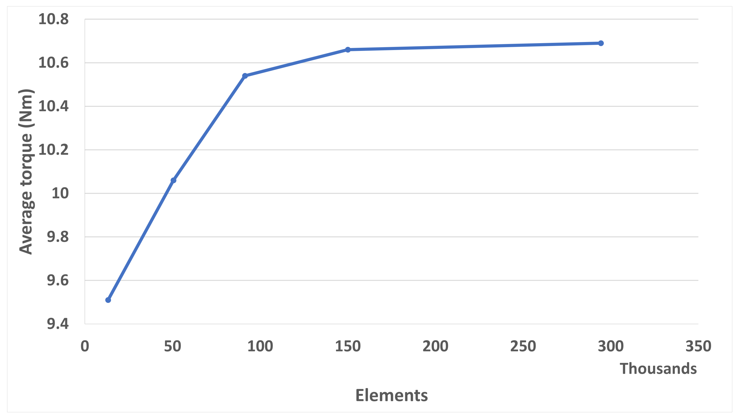
3.3. Mesh Resolution and Quality

A mesh independence study was conducted before all the design simulations to optimise the element number for the correct solution and therefore computational time. Five simulations were conducted at different mesh resolutions, starting with a coarse mesh, and increasing until a very fine mesh was created wherein the solution did not change for an increase in elements. Figure 5 shows the results of the study. The average torque becomes independent of an increase in mesh elements at ≈150,000. Hence, this value was chosen for all subsequent calculations so as not to cause unnecessary calculation times yet still provide an accurate value.

This quality of meshing used in each simulation was appropriate and sufficient per reported standards from [33,34]. The high smoothing operation when meshing was selected to achieve the highest possible meshing quality and this mesh quality was checked in each geometry. Through adherence to meshing guides [33,34], the following mesh metrics analysed were all suitable:

• Orthogonal quality guide: 0.95–1 [33].
• Aspect ratio: no larger than 5 in bulk flow, and up to 10 can be in the boundary layer [33].
• Skewness: maximum should be no higher than 0.9, but 0.95 is acceptable [34].

Table 1. Mesh quality metrics.

Mesh Metric	Min	Max	Average	Standard Deviation
Orthogonal quality	0.38138	1	0.98906	$3.816\times {10}^{-2}$
Aspect ratio	1	7.0033	1.2256	0.85156
Skewness	$1.3057\times {10}^{-10}$	0.8873	$5.2463\times {10}^{-2}$	0.10151

shows the mesh quality for the baseline simulation.

When comparing the acceptable values to values in this study, the orthogonal quality is excellent as it is between the range (0.95–1). For the aspect ratio, the maximum (worst) value is still within the maximum tolerable value for the boundary layer of 10 and this is found infrequently on blade-tip edge boundary layers. Finally, the skewness is well within the 0.95 maximum acceptable value and the average value obtained is in the range of 0–0.25, denoted as excellent.

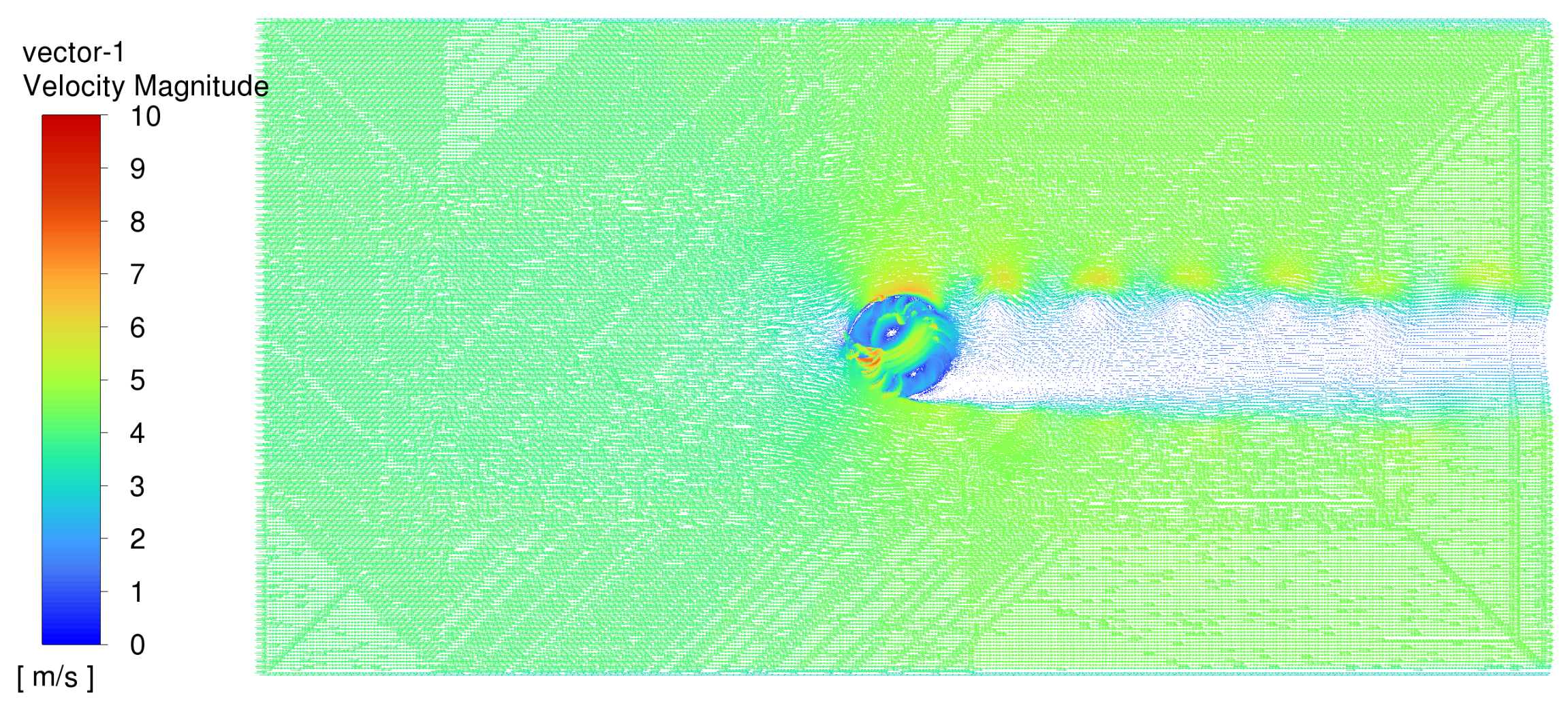
3.4. Data Extraction and Handling

After each simulation, a momentum file is generated which can be extracted and transferred to Microsoft Excel. Here, the data are initially separated into three columns: Timestep, momentum and flow-time. This is 400 timesteps long and the averages are calculated from timestep 50 to 400 as this excludes the initial time taken for the solution to stabilise. All VAWTs are fundamentally prone to torque ripple [35] which can be seen in Figure 6. The results show that the simulation does not reach steady state which is as expected because the torque varies as a function of the azimuthal position of the blades due to the varying amount of ‘captured’ air that the blade will achieve at different orientations to the incoming flow. Hence, average values of torque and power are calculated as there is no peak instantaneous power for constant inlet air, thus averaging allows for the whole performance to be quantified.

The repeating torque ripple pattern is characteristic of all simulations undertaken and shows that the simulation was stable when the same repeating peaks and troughs occur. The same process is repeated for all rotational speeds of 0.5 to 3 rad/s. Once torque and power coefficients are calculated, these are plotted with respect to TSR for each blade geometry variation to produce the results presented in Section 4.

3.5. Model Validation and Handling

The performance plots of power and torque coefficients match the trendlines seen in previous studies. The negative gradient slope for torque coefficient with respect to TSR and the ‘n’ shaped curve for the coefficient of power is similar to the peaks seen at the approximate values of about 0.5 TSR [24], and at around 0.3 TSR [29]. In this study, most geometry variations peak at a power coefficient of 0.5 TSR, although often the best performing geometries peak at higher TSR. For each geometry set apart from blade curvature angle, there have been previous studies in some form to compare results with to check the validity. For blade thickness variation, this study’s results are in line with a similar study where blade thickness is varied from 2.6 mm to 20 mm, at four intervals [18]. The same conclusion is reached wherein the thickest blade exhibits the highest power coefficient as well as the converging behaviour of each thickness for the torque vs TSR plot. For blade number variation, the study’s results match similar behaviour wherein an increase in blade number increases the performance [19,26]. However, one other study [29] finds the optimal number of blades to be 20 when considering a blade set from 16 to 24 in increments of four. The reason for this may be due to the 2 m/s inlet velocity and the blade variation being completed at 0.68 diameter ratio compared to 0.67 as well as differences in blade curvature which are undefined. It could also be argued there is evidence for this to be an optimal number of blades as the blade number against torque plot shows the 20-bladed design above the trendline. Finally, for diameter ratio, this study agrees with a prior study [29] for low blade diameter ratios of <0.6, although it finds the optimal ratio to be slightly higher. Once again, this can be explained by the slightly different setup with a 2 m/s velocity inlet and blade curvature angle difference.

4. Simulation Results

The results of the variation of each geometry are graphed for each respective set. Torque and power are investigated, both in their dimensionless and dimensioned form for a comprehensive perspective of each geometry set’s performance. Fluid behaviour is then visualised through velocity vector contours for each change in geometry.

The flow structure in the whole computational domain is presented in Figure 7:

It is evident from Figure 7 that the area directly downstream of the VAWT experiences very little airflow as shown by the lack of velocity vector contours as well as the change in colour corresponding to the scale. The areas of high velocity are seen as vortices of decreasing magnitude as they pass over the shielded part of the VAWT as well as on the initial blades that first experience the incoming air. The rest of the blades experience very little airflow when being blocked by other blades or are behind the windshield.

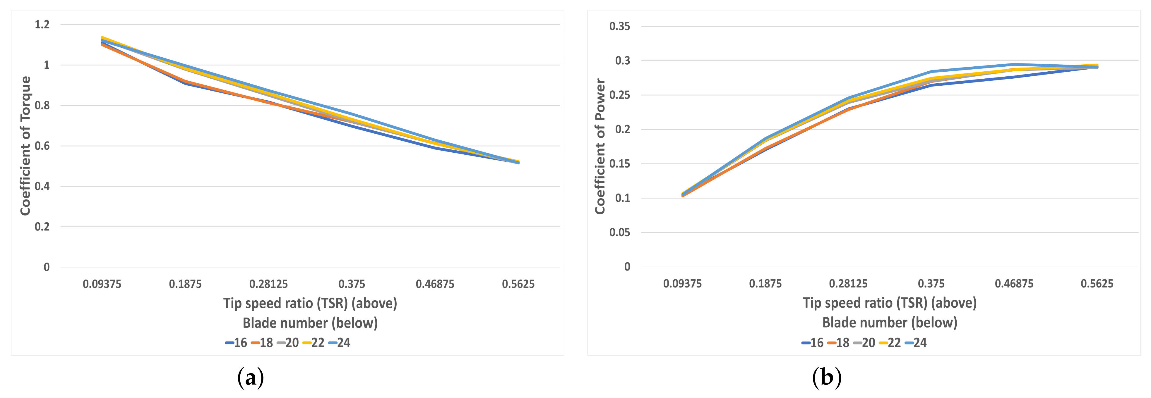
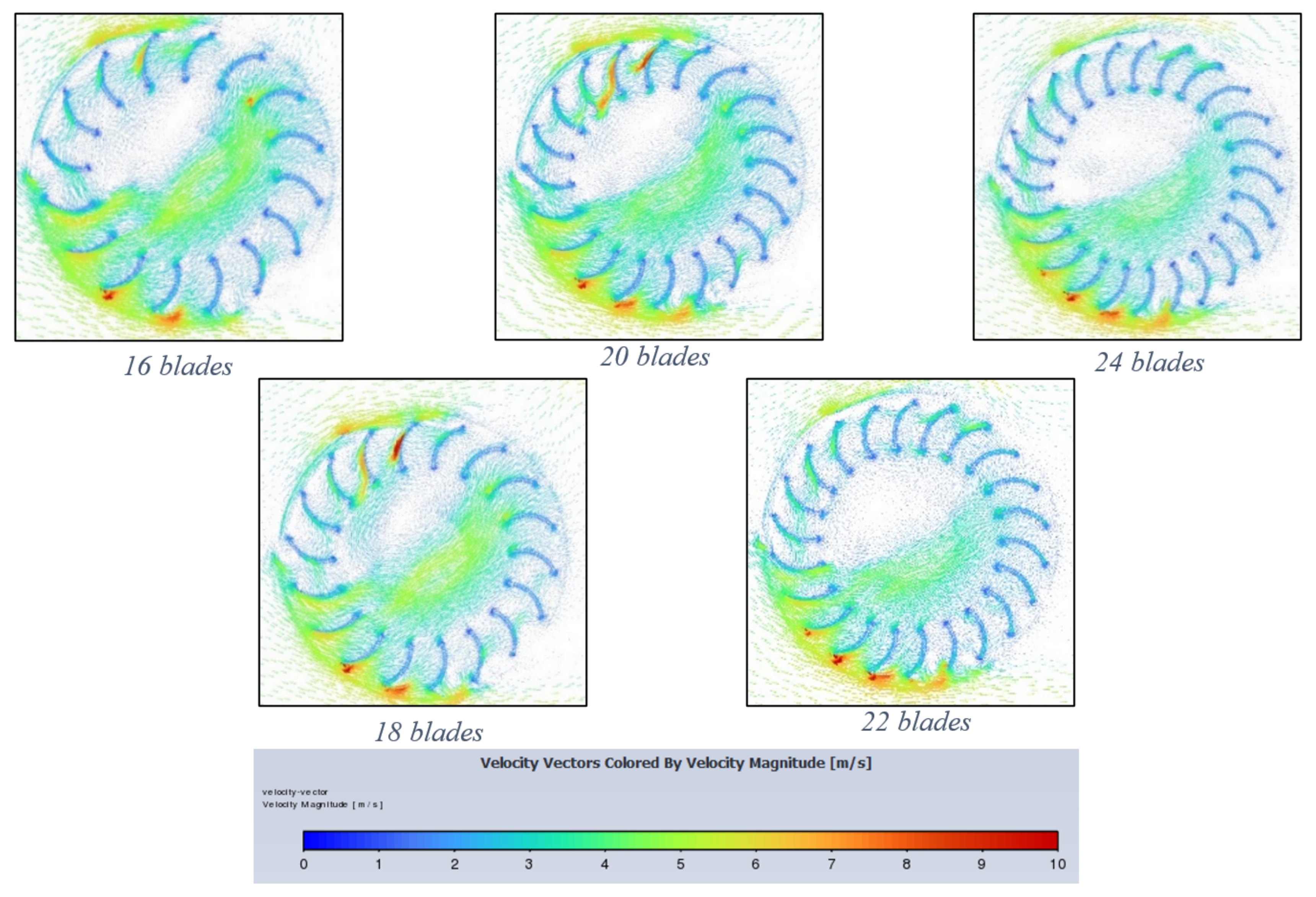
4.1. Blade Number Variation

Figure 8a shows that as blade number increase from 16 to 24 blades at increments of two blade additions, the torque increases almost linearly. Whilst the simulation with 20 blades does not break this trend, it is somewhat distant from the trendline. This could indicate that a 20-bladed design is most optimal, and this finding is also found [29]. However, the 22- and 24-bladed still outperform the 20-bladed design slightly. Figure 8b shows the peak average power (in the TSR range of the study) generation for each blade number at a rotational speed of 3 rad/s (TSR = 0.5625). As torque is closely related to the power, the trend that power generation increases with blade number is expected.

Figure 9a depicting the torque coefficient shows an almost linear decreasing negative gradient curve in which as TSR increases, the coefficient of torque also decreases. Although close, the higher the blade number, the higher the coefficient of torque apart from at low TSRs when the 22-blade turbine exhibits a higher value than 24 blades. Figure 9b shows the variation of power coefficient with respect to TSR for five different blade numbers ranging from 16 to 24 blades. All blade numbers exhibit the same positive yet decreasing gradient curve, one which levels off at around 0.5 TSR. As reported in studies [19,24,29], beyond the level-off point, the graph of the power coefficient with respect to TSR would result in an ‘n’-shaped curve, implying that the power coefficient would decrease beyond this point. Thus, it can be stated that this is a maximum value and therefore an optimal TSR. A broader range of TSR above 0.5625 would be required to confirm this.

Figure 10 exhibits flow behaviour at the end of a 400-timestep simulation at 3 rad/s (TSR = 0.5625). From these figures, the effect of the windshield is crucial in improving the overall torque and preventing negative torque. By analysing the biggest difference, which occurs between 16 and 24 blades, it can be seen that the 16-bladed turbine allows more airflow through its interior, as shown by a larger and faster region of airflow. For the 24-bladed, (top right) this region is less defined, implying that more airflow is captured by each blade. The fundamental effect of an increase in blade number from the simulation results is that torque and power increases. This is likely due to the increased catchment area that additional blades provide, thus creating a greater summation of moments about the axis centre. Whilst this increase likely invokes greater negative torque on the convex side of the blade, this is outweighed by the same increase but on the favourable concave side, which acts to catch the airflow and produce greater torque than the convex side.

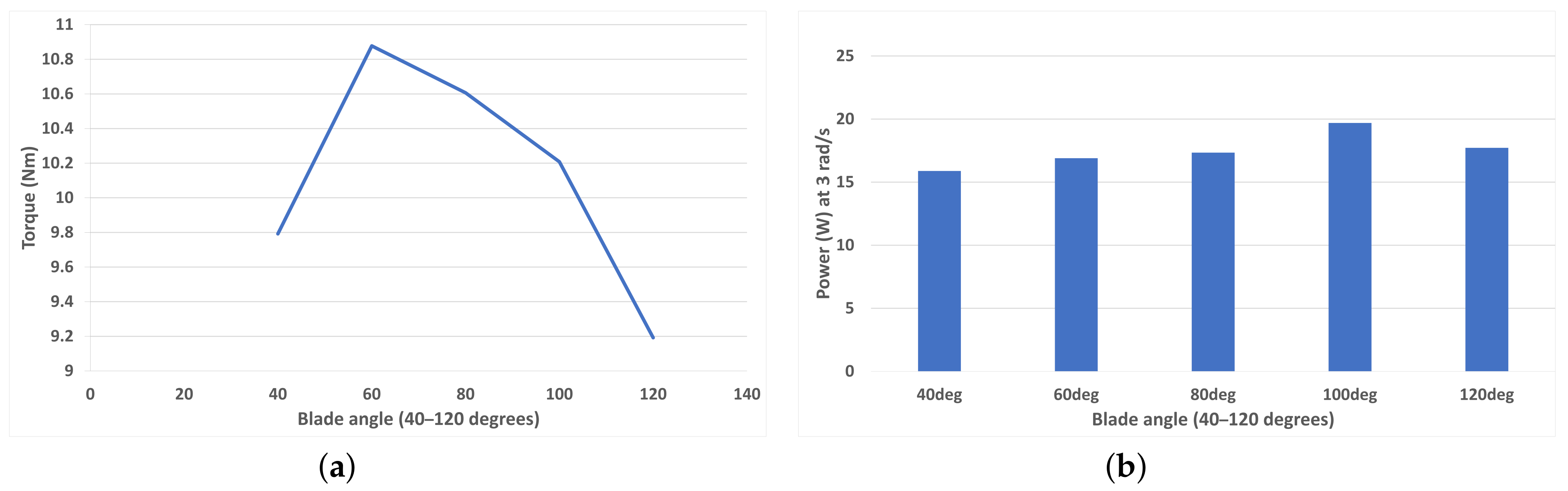
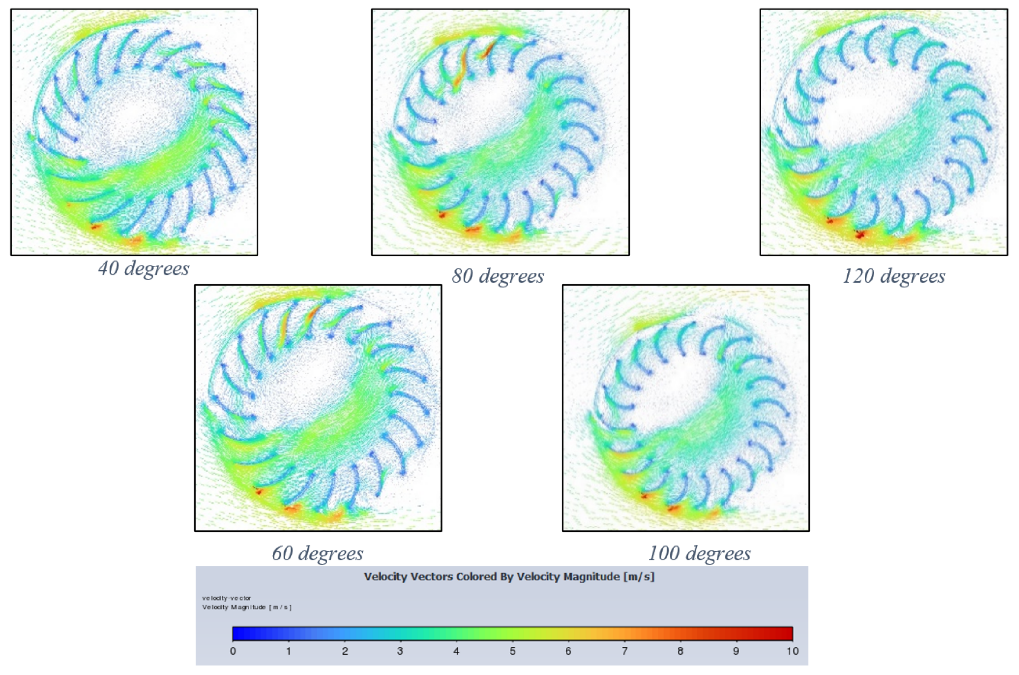
4.2. Blade Curvature Angle Variation

Figure 11a shows that as blade curvature angle curvature increases from 40 degrees to 120 degrees in 20-degree increments, there is an optimal region at around 60–70 degrees for a rotational speed of 1 rad/s (TSR = 0.1875). This torque value is lowest at high curvatures with the 120-degree blades exhibiting the worst performance. Figure 11b shows the peak average power (in the TSR range of the study) generation. It is apparent that at a faster rotational speed, the turbine with blades at 100 degrees performed best at 19.7 W power generation.

Figure 12a investigates the variation of the average torque coefficient with respect to TSR for five different blade curvature angles. As expected from the previous figures, the same trend can be seen wherein at high TSR, the turbine with blades at 60 degrees perform best at low TSR. However, at 0.25 TSR and above, the 100-degree turbine outperforms all others, with the 120-degree turbine going from the worst performing angle at slow rotational speeds to the second best at TSR = 0.5625. Figure 12b shows the variation in power coefficient with respect to TSR for blade-angle curvatures from 40 degrees to 120 degrees. Once again, the curve for all blade curvature angles shows a positive yet decreasing gradient for power coefficient versus TSR. It can be reasoned that for TSRs increasing past 0.6, the plot would peak and trail off in a symmetrical fashion. However, whilst the maximum power coefficient is almost reached for all blade curvature angles, the 100-degree turbine was yet to level off and would likely peak at a higher TSR than the others.

Figure 13 exhibits flow behaviour for blade-angle curvatures at the end of a 400 timestep, 3 rad/s simulation. Initially, at 40-degrees curvature, the blades do little to capture incoming air and optimally should function like scoops to create the most positive drag and therefore produce the highest torque. In the 120-degree curvature, which has the smallest and slowest region internally, the extreme curvature seems to produce negative torque, especially for blades at centre height on the inlet side. Therefore, whilst optimal curvature occurs at different TSRs, optimum behaviour in terms of torque and power produced is exhibited with the most ‘captured air’ to the least deflected air. The latter is characteristic of extreme curvatures.

4.3. Blade Thickness Variation

Figure 14a shows that as blade thickness increases, from 5 mm to 15 mm at 2.5 mm increments, the torque increases almost linearly for a rotational speed of 1 rad/s (TSR = 0.1875). This same result is reported in [19] and is explained by a thicker blade ‘capturing’ and impeding more of the incoming air. In line with the torque curve, Figure 14b shows that peak average power increases with blade thickness at 3 rad/s (TSR = 0.5625). As the power increase is not exponential and follows a law of diminishing gains, it is likely that in the implementation of a real-life model, the goal would be to have blade members as thin as possible.

Figure 15a depicts the coefficient of torque for all blade thicknesses with respect to the TSR. All blades follow the same trend, with a negative gradient that becomes shallower. However, at TSR > 0.3, these curves are almost indistinguishable, likely due to the relatively small effect that changes of 2.5 mm blade thickness have. Figure 15b shows the coefficient of power for each blade thickness with respect to the TSR. The curve for all blade thicknesses levels off at TSR 0.5–0.6; therefore, this region is the optimal rotational speed for maximum power generation.

Figure 16 shows airflow behaviour for each blade thickness simulation after 400 timesteps at 3 rad/s. Due to the relative similarity in the geometric and flow behaviour, the effect is much harder to visualize from this contour. Therefore, comparisons are better explained with the data obtained prior to this plot.

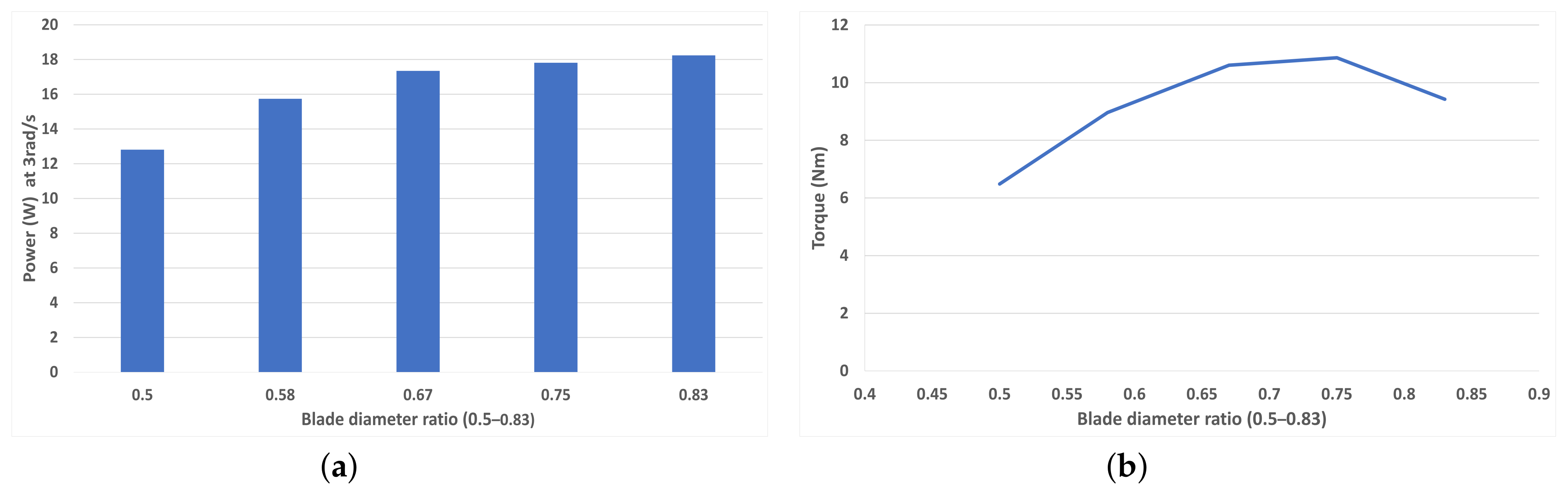
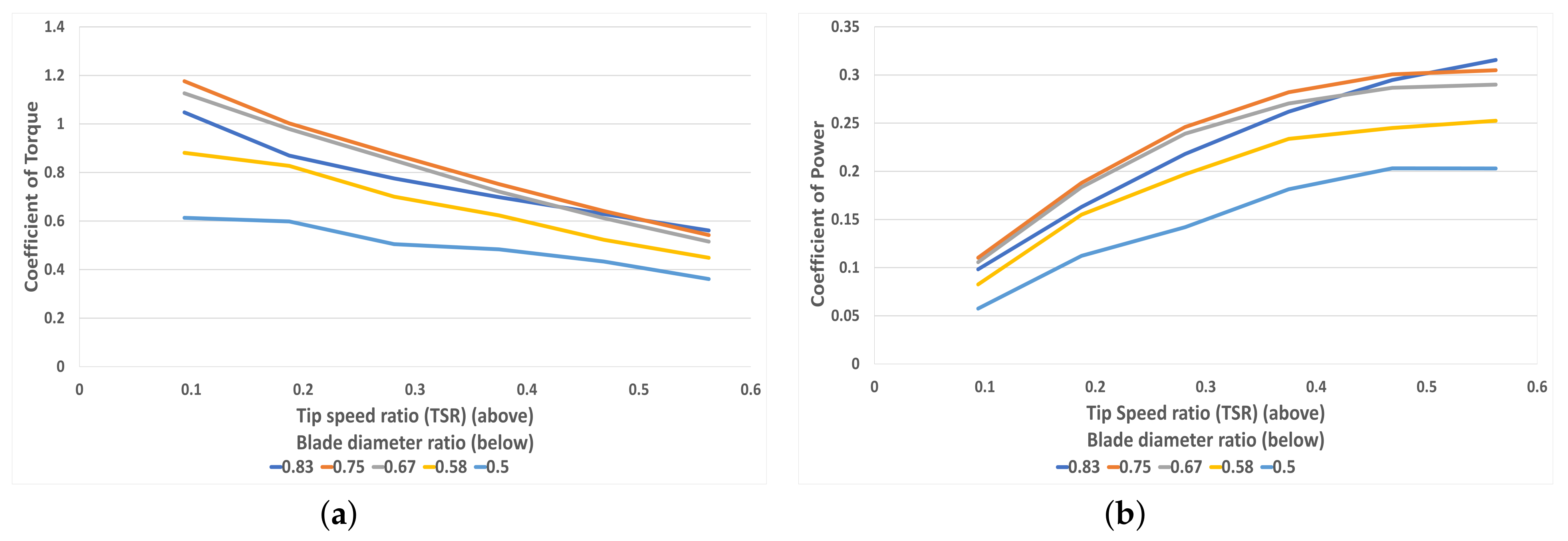
4.4. Blade Diameter Ratio Variation

Figure 17a shows that beyond and below values of diameter ratio in the range of 0.7–0.75, the torque produced trails off, suggesting that this is the optimum blade diameter ratio for 1 rad/s. Figure 17b shows peak power at 3 rad/s rotational speed. The key finding is that peak power occurs with the highest diameter ratio of 0.83 at around 18.2 W, although this is very close to the value achieved by the 0.75 diameter ratio. In a real-life scenario or a 3D simulation with inertia factored in, the weight saving of a larger diameter ratio may outweigh this difference.

Figure 18a shows the coefficient of torque for each diameter ratio with respect to TSR. Whilst the same negative gradient is seen in line with other geometries, each diameter ratio plot shows a large difference in torque coefficient compared to other geometry variations. This is due to the large difference in torque produced by each change in diameter ratio, amplified at lower ratio values. These values converge at higher TSRs, and the difference is less pronounced at fast rotational speeds. Figure 18b shows the power coefficient with respect to TSR for all blade diameter ratios. The same trend can be seen as before; however, due to the relationship between the coefficients of torque and power, the curves diverge at higher TSRs. This optimum TSR for most blade diameter ratios is reached at 0.5 TSR, except for 0.83 which was yet to peak. It can be concluded that for high rotational speeds the highest ratio is the best performing; however, at low speed the ratios 0.67 and 0.75 perform equally as well until being surpassed at 0.4 TSR.

It is apparent from Figure 19 that the higher the blade diameter ratio, the more in-flow the turbine experiences, which could be explained by the longer blades producing a shielding effect on each other. Additionally, longer blades would have more mass and, fundamentally, the section of blade closer to the turbine centre will produce less torque due to a smaller perpendicular moment arm about the centre. The inflow in the turbine centre and its blades is highest at 0.83 diameter ratio and gradually decreases for each blade diameter ratio decrease. For this ratio, the contour shows a greater number of blades experiencing substantial air velocity compared to lower velocity in lower blade diameter ratios. This will result in a greater summation of moments and therefore higher performance in terms of power and torque.

5. Discussions

The simulation results obtained from Ansys Fluent find optimal blade curvature angles which vary at different rotational speeds. Notably, at TSR = 0.1875 (low rotational speeds), the 60-degree curvature produces the highest torque. However, at TSR > 0.3 (fast rotational speeds), the 100-degree curvature is optimal, and this lead only increases with larger TSRs. Therefore, it is reasonable to say that a 100-degree curvature is suitable for turbines with higher rotational speeds and 60-degree curvature for slower rotating VAWTs. Similarly, for blade diameter ratio, an optimal value of 0.75 is found at TSR in the range of 0.1 to 0.5. However, at faster rotational speeds of TSR > 0.5, the 0.83 blade diameter ratio becomes optimal with it achieving the highest coefficient of power. For geometry variation in blade number and thickness, there is an obvious trend that when increased, the torque and therefore power increase almost linearly. However, this is only completed at fixed rotational velocities and does not factor in the mass and inertia of the turbine. Thus, it can be reasoned that increasing blade number or thickness would not be beneficial in a real-life implementation unless it was found that torque and power were exponential. This is due to a greater mass found in these geometries that has a larger rotational inertia, therefore increasing the force required to spin the turbine in a real-life model. It should be noted that from the results, a real-life installation would perform best in the range of 0.5–0.7 TSR as this is the region for which the highest coefficient of power is achieved for all setups. For this to occur, the size of the installation and the average wake speed would have to be quantified in the TSR equation as well as a system to ensure that the rotational speed stays within the optimal zone as much as possible. This could be done with a series of gears which offer more/less resistance to rotation.

The best performing geometries out of each considered geometry set in terms of power coefficient and the corresponding TSR by comparison to the baseline performance are presented in

Table 2. Peak performance in each geometry set.

Characteristic Geometry	Peak Power Coefficient	TSR	% Difference from the Baseline
24 blades	0.295	0.46875	+2.7%
15 mm thickness	0.300	0.5625	3.4%
0.83 blade diameter ratio	0.316	0.5625	+9.0%
100-degree curvature	0.331	0.5625	+14.1%

. It can be concluded from this study that the most crucial geometric parameter considered to increase energy-harvesting efficiency is the blade curvature angle with a 14% increase in power coefficient from the baseline, followed closely by the optimal blade diameter ratio at 9% increase. By extraction of each best performing geometry studied, it can be reasoned that the highest numerical performance in 2D would be achieved with a turbine of 24 blades whose members are 15 mm thick, 100-degree blade curvature and 0.83 blade diameter ratio for fast rotations. However, for slow rotations TSR < 0.4, 60-degree blade curvature and a blade diameter ratio of 0.75 is optimal. Ultimately, in a worst-case scenario for energy harvesting via a VAWT (provided there is wind), the turbine is somewhat omni-directional even with windshield(s) and can therefore still generate energy. Better still would be the advent of an automatic system which operates in low air speeds (low traffic volumes), which moves/folds away these windshields for the VAWT to take full advantage of the wind.

6. Conclusions

In summary, the investigation into various geometric parameters for enhancing Vertical Axis Wind Turbine (VAWT) efficiency has yielded valuable insights. Notably, this study underscores the pivotal role of the blade curvature angle, showcasing a remarkable 14% increase in power coefficient over the baseline, closely followed by the optimal blade diameter ratio with a 9% improvement. These findings provide crucial guidance for optimizing VAWT design, with specific recommendations for different operational scenarios and wind conditions. Ultimately, a real-life implemented VAWT would benefit through the utilisation of the optimal blade-angle curvatures found in this study. The optimal curvature captures the most wind within its blades, providing greater torque about VAWT’s centre, thereby leading to enhanced energy-harvesting capacity. For the other geometry sets, a 3D simulation would be required to come to conclusiveness due to the changes in mass that occur. In this regard, future work would include a moving mesh of two Ahmed bodies moving past a VAWT through the adoption of 3D CFD methods that accurately consider mass and inertia changes that occur through geometry variations.

References

1. Sgouridis, S.; Csala, D.; Bardi, U. The sower’s way: Quantifying the narrowing net-energy pathways to a global energy transition. Environ. Res. Lett. 2016, 11, 094009. [Google Scholar] [CrossRef]
2. Tian, W.; Mao, Z.; An, X.; Zhang, B.; Wen, H. Numerical study of energy recovery from the wakes of moving vehicles on highways by using a vertical axis wind turbine. Energy 2017, 141, 715–728. [Google Scholar] [CrossRef]
3. Tian, W.; Mao, Z.; Li, Y. Numerical Simulations of a VAWT in the Wake of a Moving Car. Energies 2017, 10, 478. [Google Scholar] [CrossRef]
4. Johari, M.K.; Jalil, M.; Shariff, M.F.M. Comparison of horizontal axis wind turbine (HAWT) and vertical axis wind turbine (VAWT). Int. J. Eng. Technol. 2018, 7, 74–80. [Google Scholar] [CrossRef]
5. Ragheb, M. Vertical Axis Wind Turbines; University of Illinois at Urbana-Champaign: Champaign, IL, USA, 2011; Volume 1. [Google Scholar]
6. Popescu, D.; Popescu, C.; Dragomirescu, A. Flow control in Banki turbines. Energy Procedia 2017, 136, 424–429. [Google Scholar] [CrossRef]
7. Quaranta, E.; Perrier, J.P.; Revelli, R. Optimal design process of crossflow Banki turbines: Literature review and novel expeditious equations. Ocean Eng. 2022, 257, 111582. [Google Scholar] [CrossRef]
8. Khosrowpanah, S.; Fiuzat, A.; Albertson, M.L. Experimental study of cross-flow turbine. J. Hydraul. Eng. 1988, 114, 299–314. [Google Scholar] [CrossRef]
9. D’Ambrosio, M.; Medaglia, M. Vertical Axis Wind Turbines: History, Technology and Applications. Master’s Thesis, Högskolan-Halmstad, Halmstad, Sweden, 2010. [Google Scholar]
10. Riegler, H. HAWT versus VAWT: Small VAWTs find a clear niche. Refocus 2003, 4, 44–46. [Google Scholar]
11. Carrigan, T.J.; Dennis, B.H.; Han, Z.X.; Wang, B.P. Aerodynamic shape optimization of a vertical-axis wind turbine using differential evolution. Int. Sch. Res. Not. 2012, 2021, 528418. [Google Scholar] [CrossRef]
12. Pope, K.; Dincer, I.; Naterer, G. Energy and exergy efficiency comparison of horizontal and vertical axis wind turbines. Renew. Energy 2010, 35, 2102–2113. [Google Scholar] [CrossRef]
13. Li, Y.; Yang, S.; Feng, F.; Tagawa, K. A review on numerical simulation based on CFD technology of aerodynamic characteristics of straight-bladed vertical axis wind turbines. Energy Rep. 2023, 9, 4360–4379. [Google Scholar] [CrossRef]
14. Somoano, M.; Huera-Huarte, F. Bio-inspired blades with local trailing edge flexibility increase the efficiency of vertical axis wind turbines. Energy Rep. 2022, 8, 3244–3250. [Google Scholar] [CrossRef]
15. Alpha 311. Available online: https://alpha-311.com/ (accessed on 10 March 2023).
16. Manathunga, D.; Karurarathna, T.; Kanchana, I.; Wettasinghe, J. Design and Development of Vertical Axis Wind Turbine for Power Generation in Expressways; University of Vocational Technology: Dehiwala-Mount Lavinia, Sri Lanka, 2021. [Google Scholar]
17. Wikantyoso, F.; Oktavitasari, D.; Tjahjana, D.; Hadi, S.; Pramujati, B. The Effect of Blade Thickness and Number of Blade to Crossflow Wind Turbine Performance using 2D CFD Simulation. Int. J. Innov. Technol. Explor. Eng. 2019, 8, 17–21. [Google Scholar]
18. Tjahjana, D.D.D.P.; Purbaningrum, P.; Hadi, S.; Wicaksono, Y.A.; Adiputra, D. The study of the influence of the diameter ratio and blade number to the performance of the cross flow wind turbine by using 2D computational fluid dynamics modeling. AIP Conf. Proc. 2018, 1931, 030034. [Google Scholar]
19. Zheng, M.; Li, Y.; Teng, H.; Hu, J.; Tian, Z.; Zhao, Y. Effect of blade number on performance of drag type vertical axis wind turbine. Appl. Sol. Energy 2016, 52, 315–320. [Google Scholar] [CrossRef]
20. Yahya, W.; Ziming, K.; Juan, W.; Qurashi, M.S.; Al-Nehari, M.; Salim, E. Influence of tilt angle and the number of guide vane blades towards the Savonius rotor performance. Energy Rep. 2021, 7, 3317–3327. [Google Scholar] [CrossRef]
21. Solidworks, 2022 Student Edition. 2022. Available online: https://www.solidworks.com/product/students (accessed on 10 March 2023).
22. Tian, W.; Song, B.; Mao, Z. Numerical investigation of wind turbines and turbine arrays on highways. Renew. Energy 2020, 147, 384–398. [Google Scholar] [CrossRef]
23. Ansys, 2022 R2 Student Edition. 2022. Available online: https://www.ansys.com/en-gb/academic/students/ansys-student (accessed on 10 March 2023).
24. Bani-Hani, E.H.; Sedaghat, A.; Al-Shemmary, M.; Hussain, A.; Alshaieb, A.; Kakoli, H. Feasibility of highway energy harvesting using a vertical axis wind turbine. Energy Eng. 2018, 115, 61–74. [Google Scholar] [CrossRef]
25. Shah, S.R.; Kumar, R.; Raahemifar, K.; Fung, A.S. Design, modeling and economic performance of a vertical axis wind turbine. Energy Rep. 2018, 4, 619–623. [Google Scholar] [CrossRef]
26. Barth, T.; Ohlberger, M. Finite Volume Methods: Foundation and Analysis; John Wiley & Sons, Ltd.: Hoboken, NJ, USA, 2003. [Google Scholar]
27. Matyushenko, A.; Garbaruk, A. Adjustment of the k-ω SST turbulence model for prediction of airfoil characteristics near stall. J. Phys. Conf. Ser. 2016, 769, 012082. [Google Scholar] [CrossRef]
28. Menter, F.R. Two-equation eddy-viscosity turbulence models for engineering applications. AIAA J. 1994, 32, 1598–1605. [Google Scholar] [CrossRef]
29. Tabib, M.; Siddiqui, M.S.; Rasheed, A.; Kvamsdal, T. Industrial scale turbine and associated wake development-comparison of RANS based Actuator Line Vs Sliding Mesh Interface Vs Multiple Reference Frame method. Energy Procedia 2017, 137, 487–496. [Google Scholar] [CrossRef]
30. Wenlong, T.; Baowei, S.; Zhaoyong, M. A numerical study on the improvement of the performance of a banki wind turbine. Wind Eng. 2014, 38, 109–116. [Google Scholar] [CrossRef]
31. Matias, I.J.T.; Danao, L.A.M.; Abuan, B.E. Numerical Investigation on the Effects of Varying the Arc length of a Windshield on the Performance of a Highway Installed Banki Wind Turbine. Fluids 2021, 6, 285. [Google Scholar] [CrossRef]
32. Ansys Fluent User’s Guide, 12.3.1 Near-Wall Mesh Guidelines; Ansys Fluent Inc.: Lebanon, NH, USA, 2009.
33. Ansys Fluent User’s Guide, 6.2.2 Mesh Quality; Ansys Fluent Inc.: Lebanon, NH, USA, 2009.
34. Ansys Mesh Quality Pdf. Available online: https://featips.com/wp-content/uploads/2021/05/Mesh-Intro_16.0_L07_Mesh_Quality_and_Advanced_Topics.pdf. (accessed on 21 April 2023).
35. Dessaint, L.; Nakra, H.; Mukhedkar, D. Propagation and elimination of torque ripple in a wind energy conversion system. IEEE Trans. Energy Convers. 1986, 104–112. [Google Scholar] [CrossRef]
Figure 1. Computational domain (all dimensions in metres).
Energies 16 07245 g001
Figure 2. Banki turbine baseline design (left), windshield design (right).
Energies 16 07245 g002
Figure 3. Each geometry set definition.
Energies 16 07245 g003
Figure 4. (top) Mesh inflation layers at boundary, (bottom) Turbine mesh.
Energies 16 07245 g004
Figure 5. Mesh independency study for 5 different mesh resolutions on the baseline design.
Energies 16 07245 g005
Figure 6. Flow time vs moment (torque) depicting torque ripple for baseline simulation at 3 rad/s.
Energies 16 07245 g006
Figure 7. Flow structure of whole computational domain.
Energies 16 07245 g007
Figure 8. (a) Average torque for each blade number (16–24) at 1 rad/s (TSR = 0.1875), (b) Peak average power for each blade number at 3 rad/s (TSR = 0.5625).
Energies 16 07245 g008
Figure 9. (a) The correlation between torque coefficient and TSR for each blade number (16–24), (b) The correlation between power coefficient and TSR for each blade number (16–24).
Energies 16 07245 g009
Figure 10. Velocity vector contours for each blade number at 3 rad/s (increasing from left to right) (16–24 blades).
Energies 16 07245 g010
Figure 11. (a) Average torque for each blade curvature angle (40–120 degrees) at 1 rad/s (TSR = 0.1875). (b) Peak average power for each blade curvature angle (40–120 degrees) at 3 rad/s (TSR = 0.5625).
Energies 16 07245 g011
Figure 12. (a) The correlation between torque coefficient and TSR for each blade curvature (40–120 degrees), (b) The correlation between power coefficient and TSR for each blade curvature (40–120 degrees).
Energies 16 07245 g012
Figure 13. Velocity vector contours for each blade curvature (40–120 degrees) decreasing from left to right.
Energies 16 07245 g013
Figure 14. (a) Average torque for each blade thickness (5–15 mm) at 1 rad/s (TSR = 0.1875), (b) Peak average power for each blade thickness (5–15 mm) at 3 rad/s (TSR = 0.5625).
Energies 16 07245 g014
Figure 15. (a) The correlation between torque coefficient and TSR for each blade thickness (5–15 mm), (b) The correlation between power coefficient and TSR for each blade thickness (5–15 mm).
Energies 16 07245 g015
Figure 16. Velocity vector contours for each blade thickness (5–15 mm) increasing from left to right.
Energies 16 07245 g016
Figure 17. (a) Average torque for each blade diameter ratio (0.5–0.83) at 1 rad/s (TSR = 0.1875), (b) Peak average power for each blade diameter ratio (0.5–0.83) at 3 rad/s (TSR = 0.5625).
Energies 16 07245 g017
Figure 18. (a) The correlation between torque coefficient and TSR for each blade diameter ratio (0.5–0.83), (b) The correlation between power coefficient and TSR for each blade diameter ratio (0.5–0.83).
Energies 16 07245 g018
Figure 19. Velocity vector contours for each blade diameter ratio (0.83–0.5) decreasing from left to right.
Energies 16 07245 g019