Abstract
Because of the control complexity of voltage source converters (VSCs), transient stability analysis of multi-VSC parallel systems is challenging, and there are still no effective methods to solve this problem. Inspired by the decoupling principle and combined with the normal form method, an innovative coupling-factor-based nonlinear decoupling (CFND) method is proposed. According to the coupling factors that can be used to evaluate the nonlinear coupling degree among different state variables, the CFND method approximately transforms a high-order nonlinear multi-VSC parallel system into multiple decoupled low-order modes. Thus, the transient stability of the original high-order multi-VSC system can be reflected indirectly by the mature inversing trajectory method and the phase plane method. The CFND method has universality, flexibility, and insensitivity to system order, and no need to construct corresponding Lyapunov functions for different nonlinear systems, breaking through the inherent limitations of traditional analysis methods. Furthermore, this paper derives a reduced-order large-signal model and the corresponding truncated model for a single VSC grid-connected system. The effectiveness of the reduced-order model is verified through simulation waveforms and ROAs partitioning. Subsequently, a generalized model of the multi-VSC grid-connected system is developed. Finally, taking the grid-connected system with three VSCs as an example, the proposed CFND method is used to analyze typical operation cases, and the conclusions of transient stability analysis are verified using the hardware-in-loop (HIL) experiments.
1. Introduction
With urgent carbon reduction requirements, an increasing number of renewable sources are integrated into the power grid through power electronic devices. Compared with the power system mainly composed of synchronous machines, the multi-voltage-source-converter (multi-VSC) parallel system lacks inherent inertia and damping, and its dynamics are more dependent on the adopted digital control algorithms. Hence, system state variables such as voltages and frequencies can be easily changed in real-time and present complex dynamic trajectories when the system suffers a large disturbance. This has led to increasing public concern about power system stability [1,2,3].
Generally, stability analysis is categorized into steady stability and transient stability, which are also known as small-signal stability and large-signal stability. Small-signal stability adopts the linear theory to analyze the system dynamics around the operation point, which mainly focuses on the ability of the system to maintain stable operation under small disturbances. There has been a variety of literature on small-signal stability analysis for a single VSC or multiple paralleled VSCs [4,5,6,7,8,9]. Eigenvalue-based [7,8] and impedance-based [9] stability analyses are conducted to verify various control strategies. However, it is not sufficient for the relatively mature small-signal stability analysis to evaluate the stability of a system that may be subjected to extreme disturbances.
In the large-signal stability analysis, the ideal analysis method is to find the exact analytical solution. However, for a high-dimensional nonlinear differential equation system, even finding an approximate solution is quite difficult. The commonly used methods for transient stability analysis of power systems can be mainly classified into numerical methods, equal area methods, Lyapunov methods, and modal analysis methods. The numerical method mainly involves establishing an accurate model for the system, using computational methods to integrate and solve differential and algebraic equations, and obtaining numerical solutions or operating trajectories for each state variable. This method has high accuracy, but it requires a lot of computational power. Especially when dealing with large-scale and high-dimensional systems, the computational complexity of numerical methods significantly increases, requiring a large number of computational resources and time. In addition, numerical methods are suitable for determining the stability of a system with a certain model and cannot conclude the stability mechanism from the perspective of physical models. Although the Lyapunov function can be used for transient stability analysis of various high-order nonlinear systems [10], in terms of stability domain judgment, the ROA obtained by the Lyapunov method is mostly elliptical, while the actual system has various forms of ROA. Therefore, as the order of transient stability analysis issues increases, the analysis results of the Lyapunov method gradually become conservative and are not suitable for the precise division of transient stability domains. The high-order modal analysis method, as a continuation of small-signal modal stability analysis methods, is an important research hotspot in the current nonlinear field. Currently, it can be mainly divided into normal form methods, Kalman linearization methods, and so on. The normal form method was initially established by Poincaré, aiming to simplify the dynamics of nonlinear systems by continuously using approximate identity transformations of coordinates, which were selected to eliminate nonresonant terms of corresponding orders. Ref. [11] proposed a normal form method that extends to the cubic term and is applied to transient stability analysis of a 2-zone 4-machine system. The Kalman linear method involves embedding a nonlinear system into an infinite dimensional linear model and analyzing it using linear theory to obtain information such as higher-order modes and nonlinear participation factors [12]. However, most of the current high-order modal analysis methods are limited to converting high-order nonlinear systems into the superposition of linear modes, and then using mature linear methods for analysis, making it difficult to provide specific ROA and effective transient stability judgment conclusions.
Due to the limitations of high-order nonlinear system transient stability analysis methods, existing work mainly focuses on the second-order model development for the single VSC and the stable region calculation. Ref. [13] develops a reduced-order nonlinear model of the VSC and clarifies the negative effect of voltage sag owing to the nonexistence of stable operation points. However, the existence of the stable operation point is only a necessary condition, and the mechanism by which the system cannot converge to the stable operation point is not revealed. Based on the reduced-order model, a PLL is considered to be the key factor of system instability, and the adoption of a low-order PLL is proposed as an adaptive control method to improve stability [14]. The equal area criterion (EAC), the improved equal area criterion (IEAC), and the Lyapunov methods are compared in [15] regarding the advantages and disadvantages as well as the accuracy of stable region estimation. The results show that the stable region obtained based on Lyapunov is relatively conservative, while the EAC may lead to an erroneous conclusion owing to ignoring the unfavorable influence of negative damping. In contrast, the stable region obtained by the IEAC is in better agreement with the simulation results. In addition, ref. [16] comprehensively summarizes the current status of transient stability analysis of a single VSC under various control modes.
The stability analysis is more difficult owing to the strong nonlinearity and complexity of dynamic interactions in multi-VSC parallel systems [4,5]. The transient stability of the paralleled synchronous and VSG (SG-VSG) system and the paralleled VSG system are analyzed and compared in [17]. However, that paper focuses on the transient stability between two machines, which cannot be easily generalized to multiple machines. In large-scale converter-based wind farms, the preconditions for the existence of steady-state operation points in the low-voltage ride-through (LVRT) process are calculated and summarized [18]. Furthermore, the innovative Lyapunov’s direct method [19] and the normal form (NF) method [20] are proposed and adopted for multi-VSC system transient stability analysis. However, the computational complexity and scalability of these two methods still need to be improved. Moreover, the nonlinear modal decoupling (NMD) method is developed to construct decoupled oscillations to analyze the initial multi-oscillation system [21]. Nonetheless, this method applies only to the conventional power grid dominated by synchronous generators and considers the multi-oscillations system whose Jacobian matrix has only complex-valued eigenvalues. In summary, transient stability analysis for power systems dominated by multiple VSCs needs to be further promoted and explored.
To fill the gap in transient stability analysis for multi-VSC parallel systems with strong nonlinear features, this paper proposes the coupling factor-based nonlinear decoupling (CFND) method to decouple the high-order nonlinear model to numerous decoupled low-order modes, where coupling factors are developed to evaluate the coupling degree between different state variables. After that, through mature analysis methods for low-order nonlinear equations, including the trajectory reversing method and the phase plane method, the transient stability of the multi-VSC parallel system can be indirectly reflected by the decoupled low-order modes. In addition, a case of a three-VSC parallel system is analyzed as an illustration for transient stability analysis, and experiments verify the results. The results show that the decoupled modes can indirectly and accurately reflect the stability of the original high-order strong coupling nonlinear system.
This paper elaborates on the proposed method and experiments through five sections. Section 2 introduces the CFND method. Section 3 develops the case studies and conducts discussions. In Section 4, hardware-in-loop (HIL) experiments are conducted to verify the theoretical analysis. Conclusions are summarized in Section 5.
2. Coupling-Factor-Based Nonlinear Decoupling Method for Stability Analysis
The conventional small-signal stability analysis methods retain only the linear characteristics of the system near the equilibrium point, which is oversimplified under large disturbances. In addition, the methods cannot provide information about the exact disturbance range that the system can tolerate. This may bring a nonnegligible error and lead to inaccurate stability conclusions. However, high-order nonlinearity poses a challenge to the evaluation of the system’s region of attraction (ROA). This section introduces the method of decoupling the high-order nonlinear equations into numerous first-order and second-order modes and reflects the original system’s ROA by numerous decoupled modes.
2.1. Linear Transformation
The state space equation of a system [11] can be established as
where represents the state variable vector of the system and is the state equations matrix of the system.
Compared with the small-signal stability analysis method, linearizing the equations around the operation point, if the dominant nonlinear features of the system can be further covered, the reliability of the stability analysis conclusion will be improved. However, the higher the nonlinear order is considered, the more limited the nonlinear analysis tools will be, and the computational complexity will increase exponentially. Hence, the degree of retention of the system nonlinearity involves a tradeoff between the reliability of the conclusion and the realizability of the analysis.
In general, retaining the nonlinear quadratic terms for typical power electronic devices can typically reflect the nonlinear characteristics of the system. For example, a constant power load and DC/DC converter are typical quadratic nonlinear systems. Thus, the nonlinear quadratic terms in the equations are retained to improve the completeness of the model, which can be represented as
where matrix is the Jacobian matrix of , represents the quadratic terms of the system and is the Hessian matrix. Similarity transformation can be performed as
where is the eigenvector matrix and represents the state variable vector after the linear transformation (also named the primary transformation). Thus, the system equations can be derived as
where matrix is the eigenvalue matrix. We define matrix ; thus, .
The systems’ small-signal stability can be determined by checking whether positive eigenvalues exist in . If the eigenvalues are positive or have a zero real part, the system is unstable or critically stable, and this conclusion is trivial. Therefore, this paper presupposes that all the system’s eigenvalues are negative. In theory, similarity transformation can be regarded as a linear decoupling method.
2.2. Classification of Variables Based on Coupling Factors
To keep the dominant nonlinear characteristics of the system and reduce the complexity of analysis as much as possible, the system is decoupled into a series of modes represented by the first- and second-order differential equations. The decoupled state equations should be of the form
where represents the state variable vector after the nonlinear quadratic transformation, and . represents polynomials of higher degree concerning . This paper assumes that the cubic term has limited influence on the stability analysis conclusion and can, therefore, be ignored.
If other state variables have limited influence on state variable , can be considered an “isolated state variable”, and the corresponding state space equation is
where the three subscripts of represent the matrix and the corresponding row and column numbers in turn.
If the coupling effect between two state variables cannot be ignored, they can be considered as a coupling pair. The equations are
Variables whose eigenvalues are complex conjugate numbers are generally considered to have strong relations and should be regarded as coupling pairs. The classification of the state variables with negative real eigenvalues depends on the coupling strength between variables, which the coupling factor can measure. The coupling factor between the state variables and can be defined as
where represents the element in the matrix and where the last two subscripts indicate the row and column numbers. In addition, and are the i-th and j-th eigenvalues of the matrix . We select the variables with the largest coupling factors from the unpaired state variables and classify them as the coupling pair. Then, the above operations are repeated until the coupling factors between the remaining variables are lower than the threshold or there is only zero or one unpaired variable left. Therefore, the state variables are classified into two categories: coupling pairs whose influence on each other cannot be omitted as (7) and isolated variables that mainly incorporate their own effects as (6).
2.3. Nonlinear Transformation Derivation
According to (4), from the perspective of primary terms, the changing trend of each state variable is related only to itself. However, the quadratic terms of different variables are still coupled together. This paper’s purpose of nonlinear decoupling is to differentiate the state variables in quadratic terms after decoupling, which cannot be obtained by a linear transformation. Consider the nonlinear transformations:
where . According to the expected decoupled state equations as (6) and (7), isolated variables incorporate only their own influence on the quadratic terms, and coupling variables incorporate only their paired variables’ influence on the quadratic terms. Therefore, uncorrelated variables should be reflected as zero in the coefficients of the quadratic terms. Moreover, to possibly preserve the original system information, the quadratic terms’ coefficients of the retained terms should be consistent with the original system, which can be expressed as (10) and (11).
For isolated state variable , the coefficients of quadratic terms are as in (10), where , .
For coupling pair variables, and , the coefficients of quadratic terms are as in (11), where and ,
Substituting (9) into (4) leads to
Combining (5) and (12), we obtain
For the quadratic terms of (13), the expression can be derived for the i-th equality of the matrix:
Expanding the above expression yields
By shifting the terms of (15), the following can be deduced:
Thus, if , the nonlinear transformation matrix can be deduced as
By nonlinear transformations as (9) and (17), the original high-order system can be decoupled into multiple low-order modes as (6) and (7), the ROA of which can be analyzed by the mature trajectory reversing method and phase plane method.
2.4. Transient Stability Assessment
Transient stability can be determined by calculating whether the initial point lies in the ROA of the steady-state operation point. According to the decoupling process described in the previous sections, the system undergoes linear transformation from the initial model in the -domain to the linear decoupling model in the -domain, and nonlinear transformation from the -domain to the nonlinear decoupling model in the -domain. The initial point in the -domain can be calculated by solving in (1). Then, similar to the process of model decoupling, it is intuitive to determine the initial point in the -domain by the similarity transformation in (3). For nonlinear transformation as (9), the initial point in the -domain can be calculated by setting as the iteration starting point through the Newton–Raphson method.
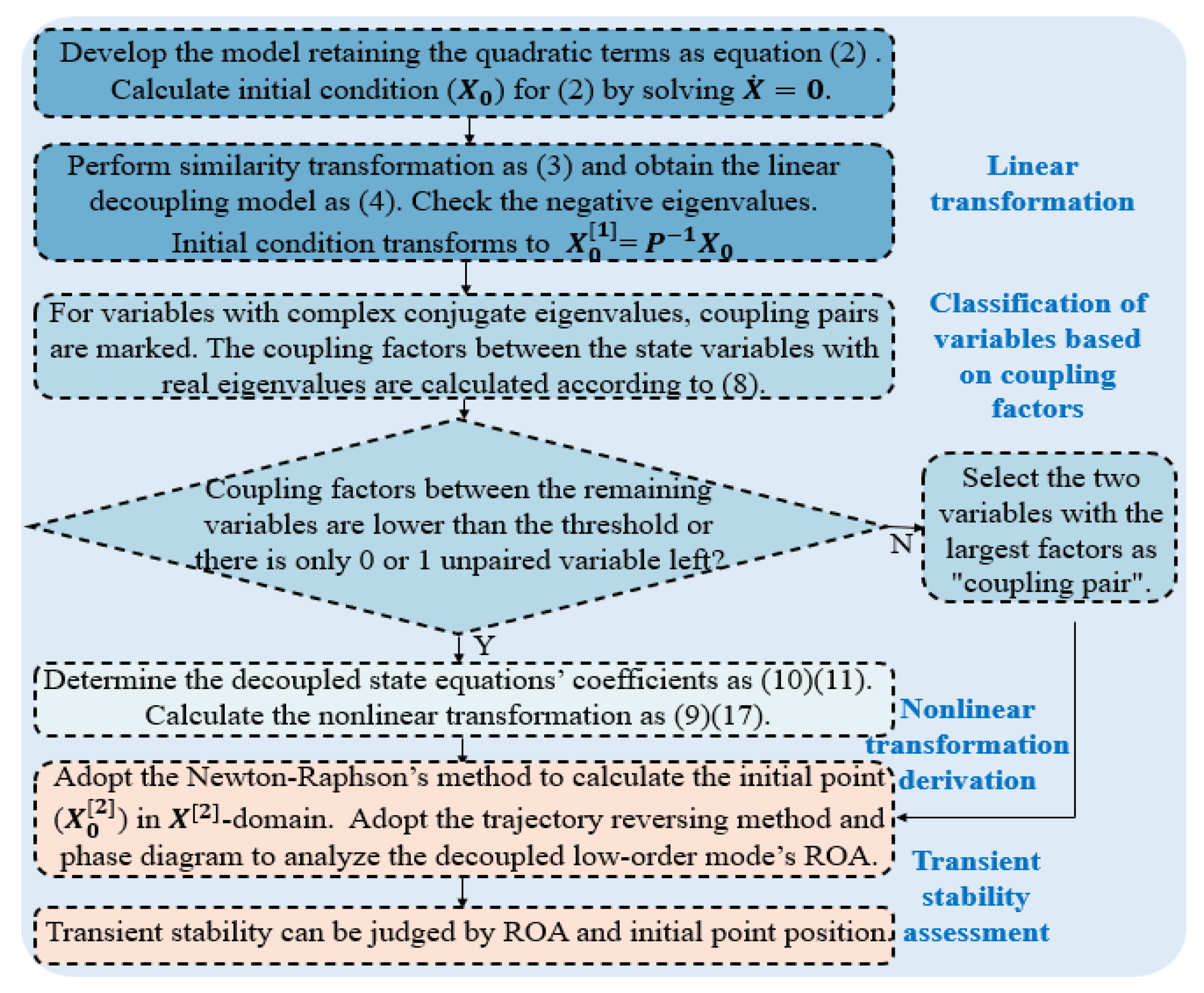
For the decoupled first-order quadratic modes in (6), the ROA can be calculated by the corresponding diagram. As shown in the diagrammatic sketch in Figure 1a, the curve intersects the abscissa axis at points a and b. When , will gradually destabilize by moving toward point a. When , also gradually moves toward point a. When , moves toward the right axis and loses stability. Upon synthesizing the derivative signs of the above three intervals, the ROA of the state variable is which means that when the initial point is in this interval, the state variable returns to the stable operating point.

Figure 1.
ROA diagrammatic sketch. (a) First-order mode. (b) Second-order mode.
For the decoupled second-order quadratic modes as (7), the ROA can be calculated by the trajectory reversing method and the phase plane method, and the diagrammatic sketch is shown in Figure 1b. If the initial point is within ROA, as with the green triangle in the figure, the mode can maintain transient stability. However, if the initial point is outside ROA, as with the red triangle in the figure, the mode is unstable.
In summary, the proposed CFND method calculates the coupling factors to evaluate the coupling degree between different variables and decouples the original high-order nonlinear system into multiple low-order quadratic modes. Thus, mature methods can be adopted to analyze the low-order modes, and the transient stability of the initial system can be reflected indirectly. The complete flow chart of the CFND method is summarized in Figure 2.
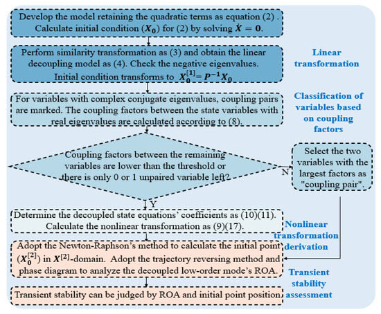
Figure 2.
Flow chart for the nonlinear decoupling stability analysis method.
3. Modeling and Transient Stability Analysis for a Multi-VSC Parallel System
3.1. System Description and Mathematical Model of the Single VSC
In this paper, the transient stability of the multi-VSC parallel system is targeted. To coherently derive a reduced order model for the multi-VSC parallel system, taking a single VSC grid-connected system as an example, the topology and control strategy of the adopted grid-following VSC are introduced, and the reduced-order model of the single VSC is obtained.
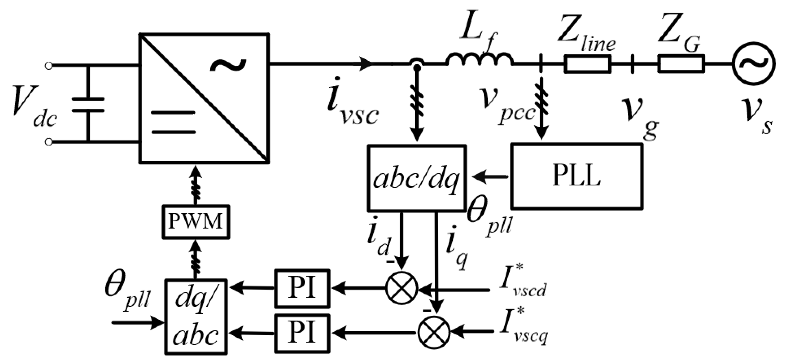
Figure 3 represents the simplified diagram and the adopted control method for each VSC. For VSC in grid-following mode, there is usually a large capacitor or a control part adopted to stabilize the DC voltage, so the DC side can be considered an ideal voltage source, the voltage of which can be represented as On the AC side, the VSC is filtered by the inductor (). After that, the VSC is connected to the weak grid by line impedance (). The weak grid consists of the ideal voltage source () and grid impedance (). The amplitude and phase of the grid voltage can be represented as and , respectively. In terms of the control strategy, the VSC measures the three-phase current () and the point of common coupling (PCC) voltage () to the PLL to obtain a phase . Through Park transformation, can be transferred to the active current () and the reactive current (). The active current reference is , and the reactive current reference is . The current is regulated by the PI controller to achieve zero-steady-state error.
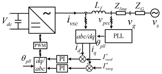
Figure 3.
Simplified single-line diagram and the adopted control method of VSC. Steady-state values are marked with *.
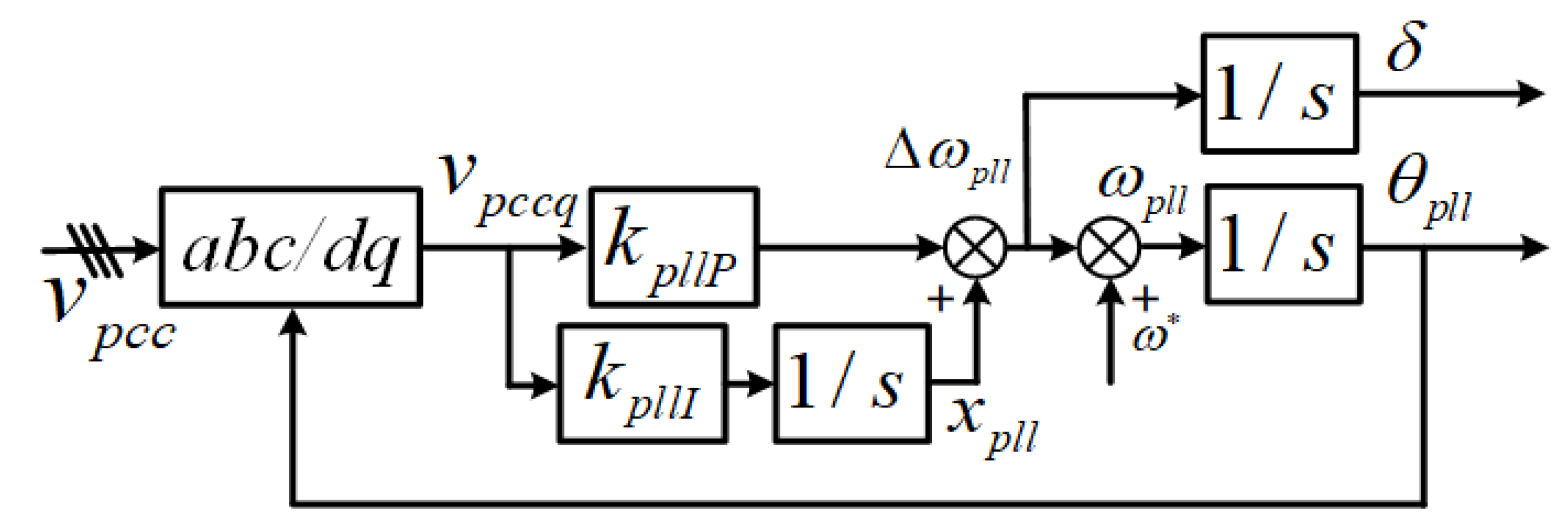
Figure 4 shows the control principle of the PLL, where and represent the proportional and integral parameters of the PI controller. Due to the presence of PI control and frequency integration, the disturbance of will be transmitted to through two integrators. Therefore, the PLL cannot achieve instant phase locking. In addition, due to the presence of line impedance and weak grid impedance, there is complex coupling between different parallel VSCs as well as between the VSC and the grid, making the transient stability analysis of multi-VSC systems more complex.
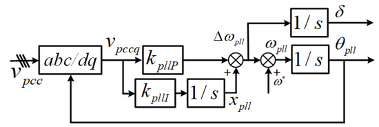
Figure 4.
Block diagram of the PLL control. Steady-state values are marked with *.
To facilitate modeling, the amplitude and phase representation is used for impedance, voltage, and current, which can be represented as
The utility grid composed of an ideal voltage source and grid impedance in series can be converted into the current source form, where
The bus voltage can be represented as
Thus, the voltage of the PCC can be represented as
For simplification, define
Combining (18)–(24), the projection of PCC voltage on the phase-locked angle can be derived as
where is the angular frequency and is the rated angular frequency value. indicates the deviation between the system frequency and the rated frequency. Power angle () can be defined as
The control principle of PLL is to achieve phase lock using a PI controller to make the projection value of the q-axis PCC voltage zero. The q-axis voltage can be derived as follows:
where represents taking the imaginary part. Generally, the system frequency is relatively close to the rated frequency, thus
When displays the inductive characteristic, and . When displays the capacitive characteristic, and
To simplify the expression and highlight the components of the q-axis voltage projection value, define the constant component as , thus the q-axis PCC voltage can be represented as
According to the PLL control principle shown in Figure 4, the state-space model can be represented as
where is the space variable introduced by the PLL integrator controller.
According to (26), considering the PLL control strategy, expressions about power angle can be derived as
Combining (29) and (31), this can be derived:
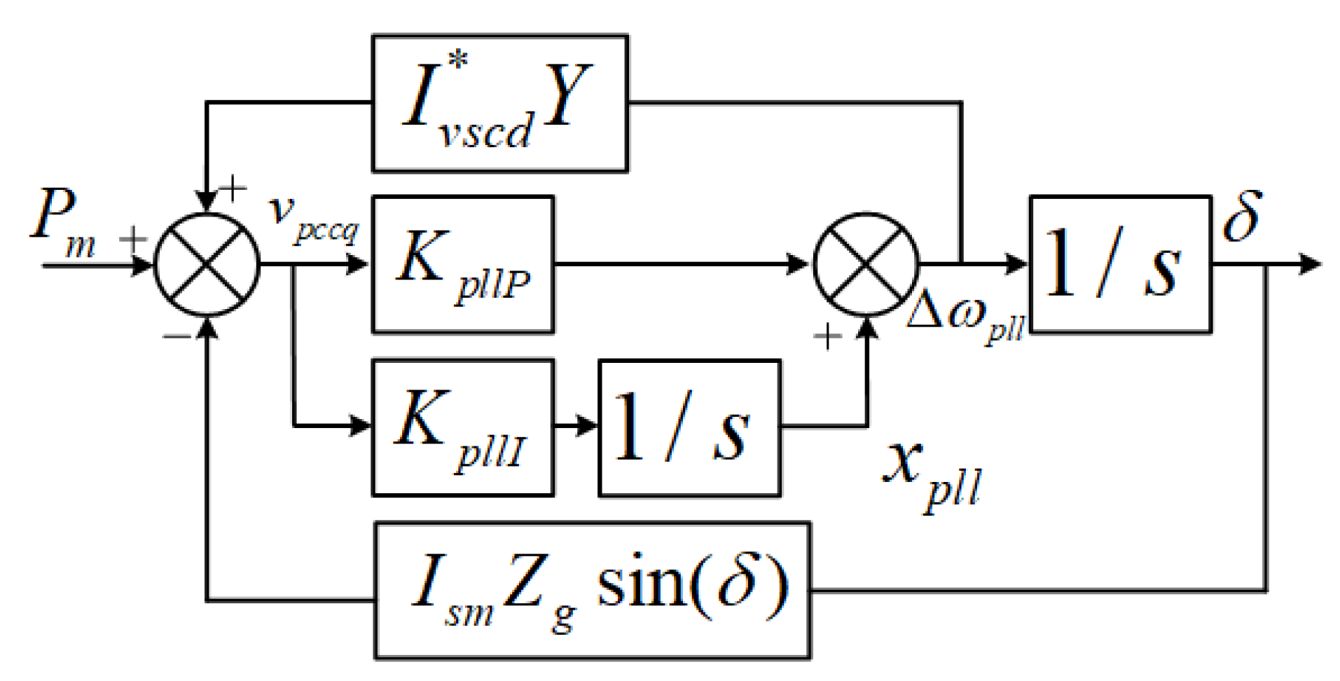
Combining (30)–(32), the reduced-order big-signal model for the single VSC system can be developed as
The big-signal model can be represented in Figure 5.
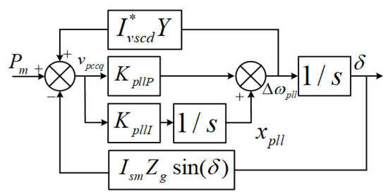
Figure 5.
Block diagram of the reduced-order big-signal model for the single VSC system. Steady-state values are marked with *.
Trigonometric functions in large-signal models pose challenges for transient stability analysis. Consequently, Taylor expansion is applied to derive the second-order and cubic-order truncated models based on the reduced-order large-signal model.
The state variable can be expressed as a combination of the steady-state quantity and the incremental value, as , where and represent the steady-state and the incremental value, respectively. Taylor’s expression about the trigonometric function is as follows:
where coefficients are .
Combining (33) and (34) by truncating the system model to the quadratic term from the steady-state operating point, the reduced-order quadratic truncation model for a single VSC grid-connected system can be derived as follows:
Similarly, by truncating the system model to the cubic term, the reduced-order cubic truncation model for a single VSC grid-connected system can be derived as follows:
Thus, the reduced-order large-signal model, along with the corresponding quadratic and cubic truncation models, for the single VSC grid-connected system is derived.
In the case of single VSC grid-connected systems, the reduced-order large-signal model is second-order, enabling direct application of mature phase diagram or inverse trajectory methods for transient stability analysis. However, as the number of VSC devices connected to the system increases, the number of system nodes grows, and the system order increases significantly. Consequently, the phase diagram method and inverse trajectory method used for analyzing low-order systems cannot be directly applied to assess the transient stability of the system.
3.2. Performance Verification for the Reduced-Order Model
To verify the effectiveness of the reduced-order model for the single VSC grid-connected system, in the case when grid voltage drops suddenly from 311 V to 31.1 V, the model can be verified by comparing response curves of the power angle, system frequency, and q-axis voltage (), adopting the accurate switch tube model and the reduced-order model through simulation. Simulation comparison diagrams are shown in Figure 6.
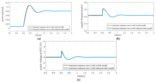
Figure 6.
Simulation comparison diagrams with switch tube model and reduced-order model when grid voltage drops from 311 V to 31.1 V. (a) Power angle curves. (b) Angular frequency curves. (c) Q-axis voltage at PCC.
According to Figure 6, when the voltage amplitude of the power grid abruptly decreases from 311 V to 31.1 V, the reduced-order model exhibits notable correspondence and robust consistency with the simulation waveforms of the switch tube model. This suggests that the reduced-order model adequately captures the dynamics of the original system. Consequently, when conducting transient stability analysis on system-level entities, employing a reduced-order model for the analysis of system transient stability is feasible, given that the control bandwidth distinction between the inner and outer loops is sufficiently large.
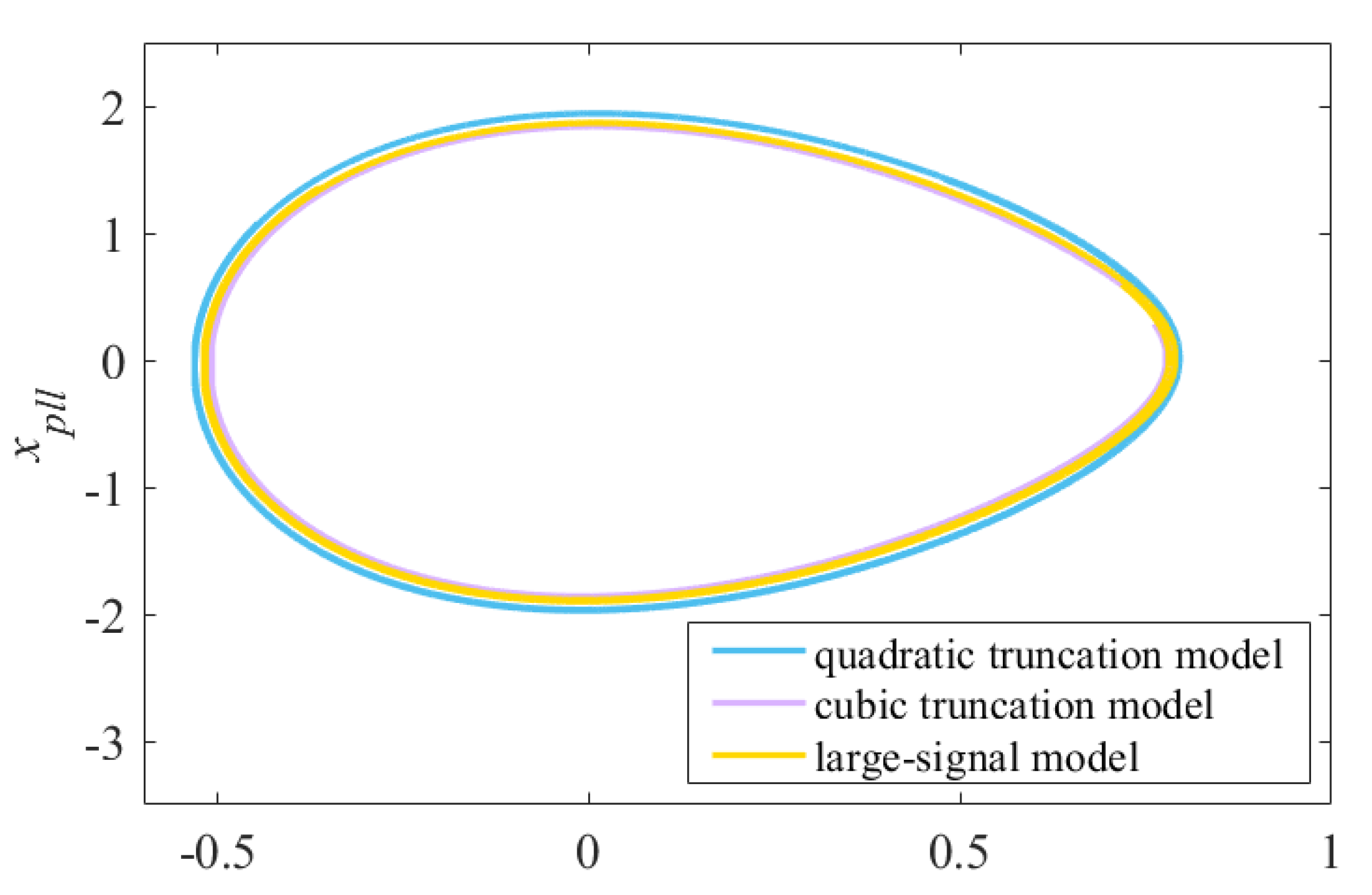
In addition, the ROAs are obtained using the mature inverse trajectory method based on the reduced-order large-signal model, quadratic truncation model, and cubic truncation model. The comparison curves can be observed in Figure 7.
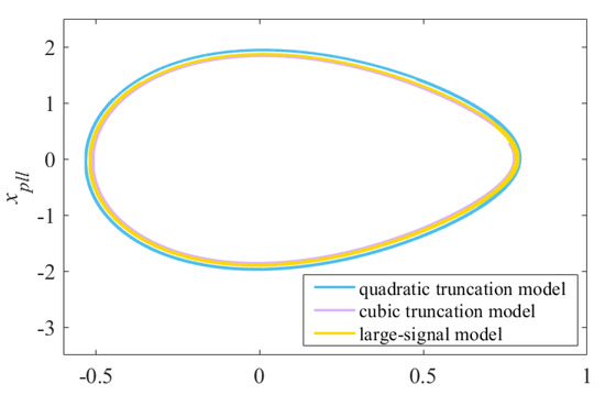
Figure 7.
Comparison of ROAs obtained using the large-signal model, quadratic truncation model, and cubic truncation model.
Figure 7 illustrates the ROAs obtained from the reduced-order large-signal model (yellow curve), quadratic truncation model (blue curve), and cubic truncation model (purple curve) for the single VSC grid-connected system. The ROAs represented by these curves exhibit significant proximity, indicating the potential use of a truncated model for simulating system characteristics and conducting transient stability analysis. Additionally, the boundaries of the ROAs obtained from the quadratic and cubic truncation models closely align with the inner and outer boundaries of the ROA obtained from the large signal model, respectively, which suggests a high degree of overlapping. Consequently, adopting the quadratic truncation model not only reduces computational complexity but also ensures adequate fitting accuracy.
3.3. Reduced-Order Derivation for the Multi-VSC Parallel System
Currently, most renewable energy sources are connected to the power grid through grid-following VSCs. Thus, this paper primarily focuses on modeling and transient stability analysis for scenarios involving multiple grid-following VSCs connected to the grid. Since the VSCs employ a similar control strategy, the circuit model and control strategy of multi-VSCs connected to the grid will not be extensively discussed further. Each grid-connected VSC will be labeled sequentially as ,. The symbol representation of circuit parameters and control parameters in a multi-VSC grid-connected system follows the same as those defined in a single VSC grid-connected system. and respectively denote the filtering inductance and line impedance associated with the k-th VSC circuit. Other parameters follow a similar pattern and will not be reiterated. To simplify the circuit topology of a multi-VSC grid-connected system, a similar circuit transformation is employed to convert the series combination of the ideal voltage source and grid impedance into a current source form. Figure 8 presents the corresponding schematic for the simplified circuit topology of the multi-VSC grid-connected system.
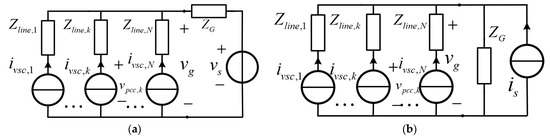
Figure 8.
Simplified system for the transient stability analysis. (a) Simplified structure diagram of the multi-VSC parallel system. (b) Equivalent circuit.
Bus voltage in the multi-VSC grid-connected system can be derived as
The measured voltage at the PCC of each VSC, which is used for the PLL of each VSC itself, can be expressed as
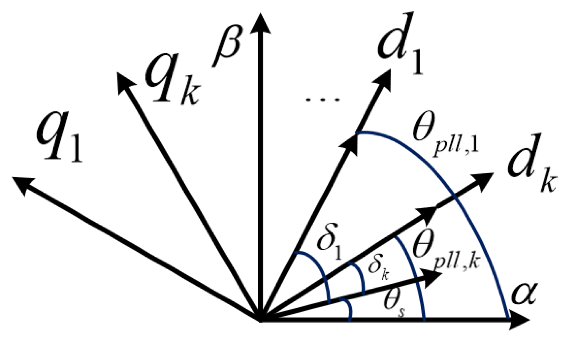
Each VSC’s PLL is regulated by locally measuring voltage information. As a result of different line impedances, the active and reactive current reference values for VSCs and angles detected by VSCs are different. Figure 9 displays the phase angle diagram for the grid-connected system with multiple VSCs.
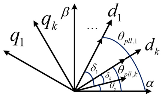
Figure 9.
Diagram of power angles in the multi-VSC grid-connected system.
For simplification, define
Thus, the voltage of PCC can be derived as
The control principle of the PLL in each VSC involves using a PI controller to make the q-axis voltage zero, ultimately determining the phase at PCC. Therefore, the q-axis voltage at each PCC can be expressed as
Thus, the q-axis voltage can be derived as
where represents the power angle of the k-th VSC. According to (42), the PCC voltage of the k-th VSC is influenced not only by its own loop’s current reference value as well as the grid current and grid impedance but also by the current and impedance on other VSC lines. It is illustrated that coupling of the frequency and phase between multiple VSCs occurs and that the complexity of the whole system is dramatically improved.
In the multi-VSC grid-connected system, considering the control principle of PLL, similar state-space model can be developed for the k-th VSC:
where represents the state variable introduced by the integrator controller in the k-th VSC.
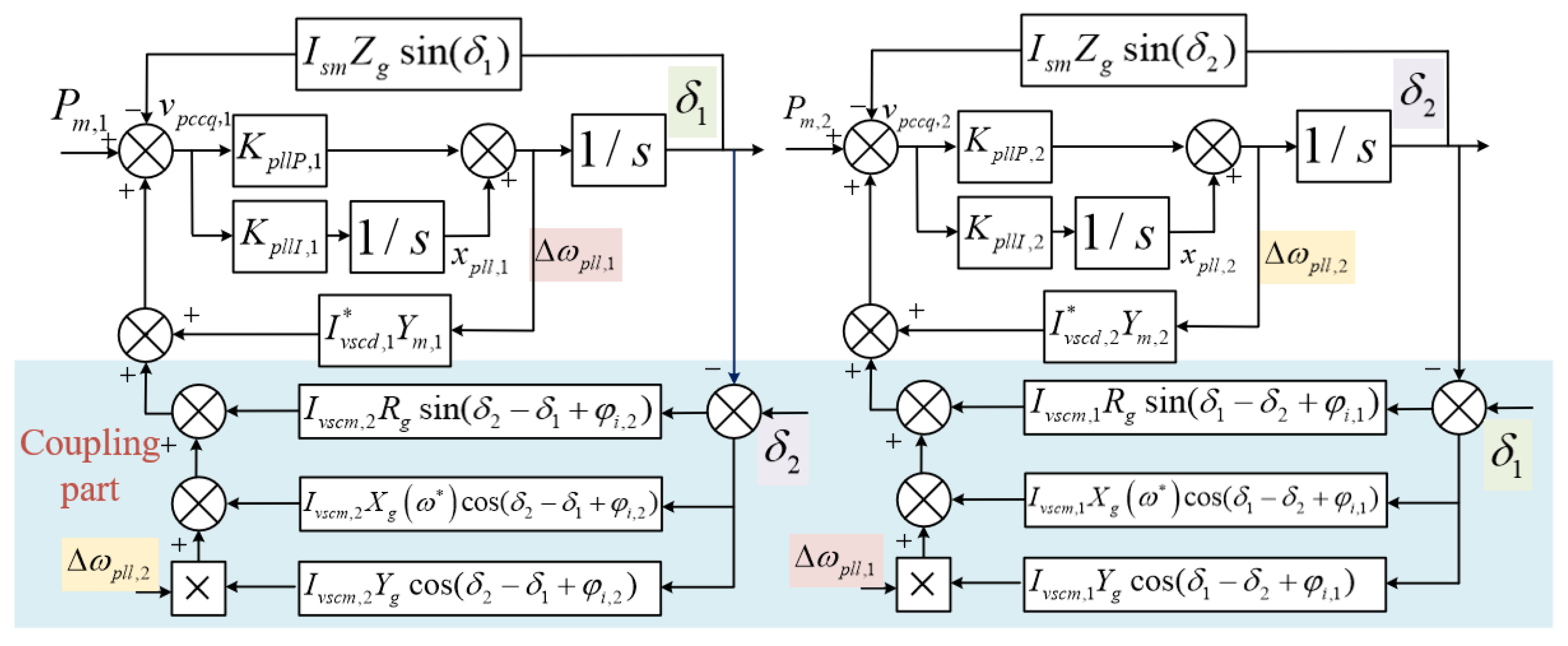
Taking the example of a grid-connected system comprising two VSCs, the corresponding large-signal block diagram is depicted in Figure 10.
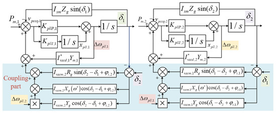
Figure 10.
Large-signal block diagram of the grid-connected system comprising two VSCs. Steady-state values are marked with *.
The multi-VSC grid-connected system, as depicted in Figure 10, exhibits high-order nonlinear characteristics and involves complex phase angle nonlinear coupling in its large signal model. Their inherent traits pose challenges in directly analyzing the transient stability of the multi-VSC parallel system.
3.4. System Transient Stability Analysis Based on CFND
This paper illustrates a three-VSC parallel system to analyze the transient stability. All state variables can be expressed as steady-state quantities (denoted by the symbol ) superimposed on the variable quantities (denoted by ), such as . Taylor expansion can be utilized for a model approximation when dealing with nonlinear functions, such as trigonometric functions, in large-signal models. Due to the comparison of the ROAs obtained from the single VSC reduced-order model and the quadratic and cubic truncation models in the previous section, it is shown that truncating to the quadratic term is sufficient to reflect the characteristics of the original system. Therefore, in the analysis of the multi-VSC grid-connected system, the truncated to quadratic Taylor expansion is used for model approximation. The relevant expansion equations are
In general, the frequency difference of VSCs in the system is slight. For simplification, if , it can be derived that . When is inductive, , where is the equivalent inductance. When is capacitive, , where is the equivalent capacitance [22]. For the sake of simplification, this paper mainly addresses the transient stability problem with slow outer loop dynamic characteristics, thus ignoring the influence of the fast current inner loop and the line dynamics [17]. Combining (42), (44) and (45), the expression of the PCC point voltage truncated to the quadratic term after Taylor transformation is as follows:
Combining (43) and (46), the nonlinear model truncated to the quadratic term of the three-VSC parallel system is developed. The form of the model is (2), and the proposed nonlinear decoupling method is utilized for stability analysis. The parameters adopted by the system are shown in Table 1. The state variables of the system can be expressed as

Table 1.
Parameters of the system.
To verify the proposed method’s effectiveness, transient stability assessments are conducted for three cases with different operation points.
CASE I: For the case when the grid voltage amplitude suddenly drops from 311 V (1.0 pu) to 31.1 V (0.1 pu), the state equations after decoupling can be obtained, and the initial operation point () can be calculated, as shown in the Table 2.
Table 2.
Initial operation points for different operation statuses.
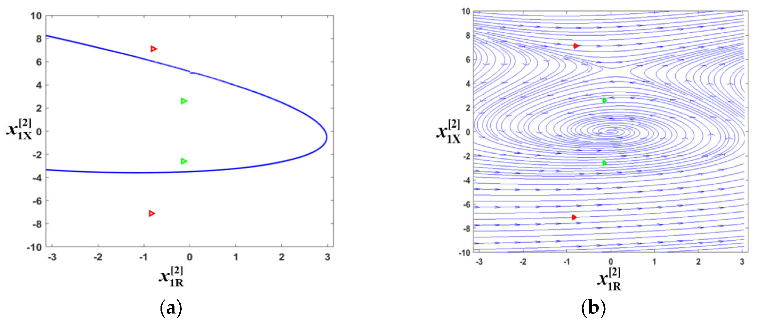
Since most of the coefficients in decoupled equations are complex, separating the real and imaginary parts for stability analysis in the real number domain is helpful. For quadratic differential equations, the mature trajectory reversing method and the phase diagram can be used to obtain the ROA.
The ROA of the coupling pair is shown inside the blue curve in Figure 11a, and the phase diagram is shown in Figure 11b. The system gradually stabilizes when the initial point lies within the blue curve range. Conversely, when the initial point is outside the ROA, the system diverges and cannot be stabilized. As Figure 11 shows, the two initial points are marked by red triangles outside the stability region, so the analysis illustrates that the system faces large-signal instability when the voltage drops from 311 V to 31.1 V.
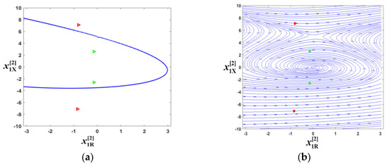
Figure 11.
Transient stability analysis of the coupling pair and the initial points for 311 V to 31.1 V (in red) and 40 V to 31.1 V (in green). (a) ROA. (b) Phase diagram.
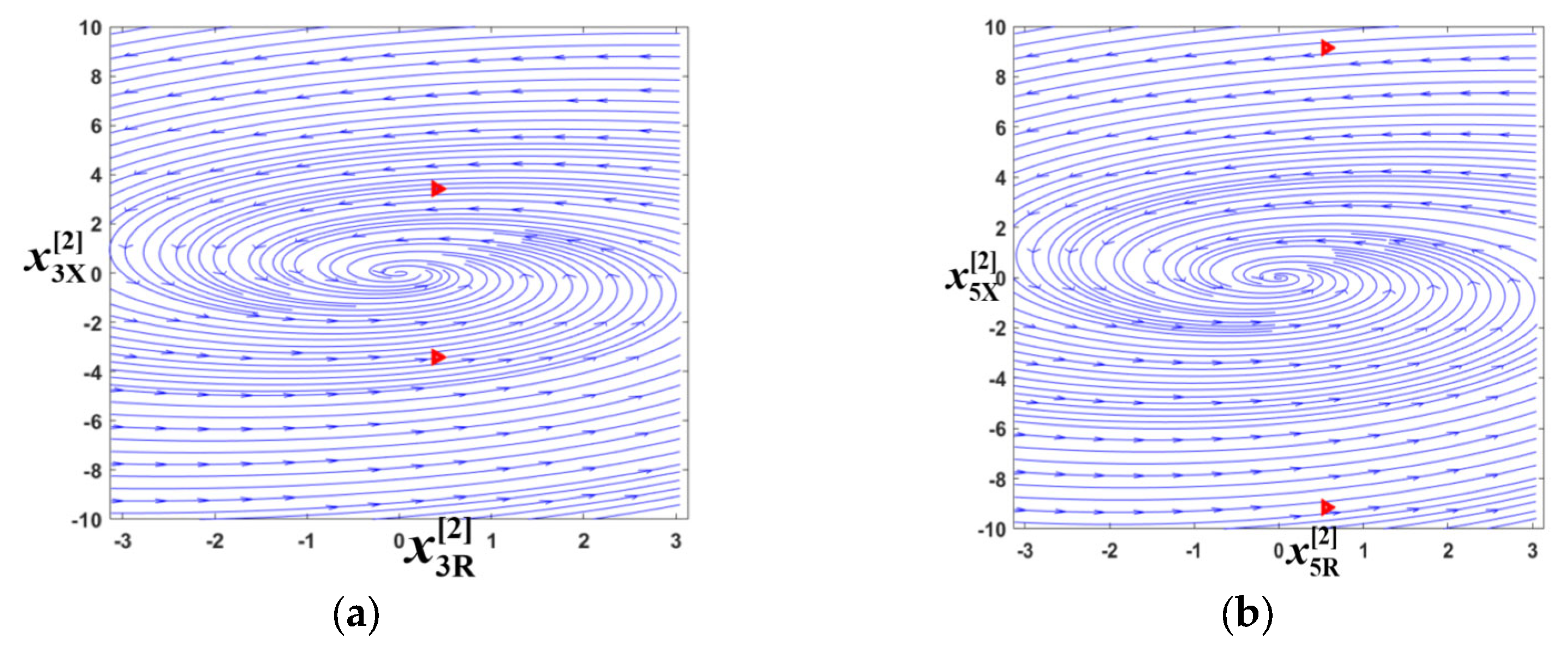
Furthermore, the phase diagrams of the coupling pairs and , and , as well as the corresponding initial points, are shown in Figure 12. The phase diagrams illustrate that these two pairs of state variables are globally stable.
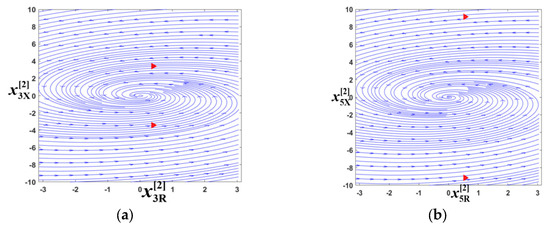
Figure 12.
Phase diagrams and the initial points for 311 V to 31.1 V. (a) Coupling pairs (b) Coupling pairs .
CASE II: For the situation when the grid voltage amplitude drops from 40 V to 31.1 V, the system parameters and steady-state operation point are the same as in case I. Therefore, the ROAs corresponding to the two cases are consistent.
As shown in Figure 11a,b, the green triangles indicate the initial points when the grid voltage amplitude drops from 40 V to 31.1 V. It can be concluded that the initial points are inside the ROA. Thus, there will be no instability when the grid amplitude drops from 40 V.
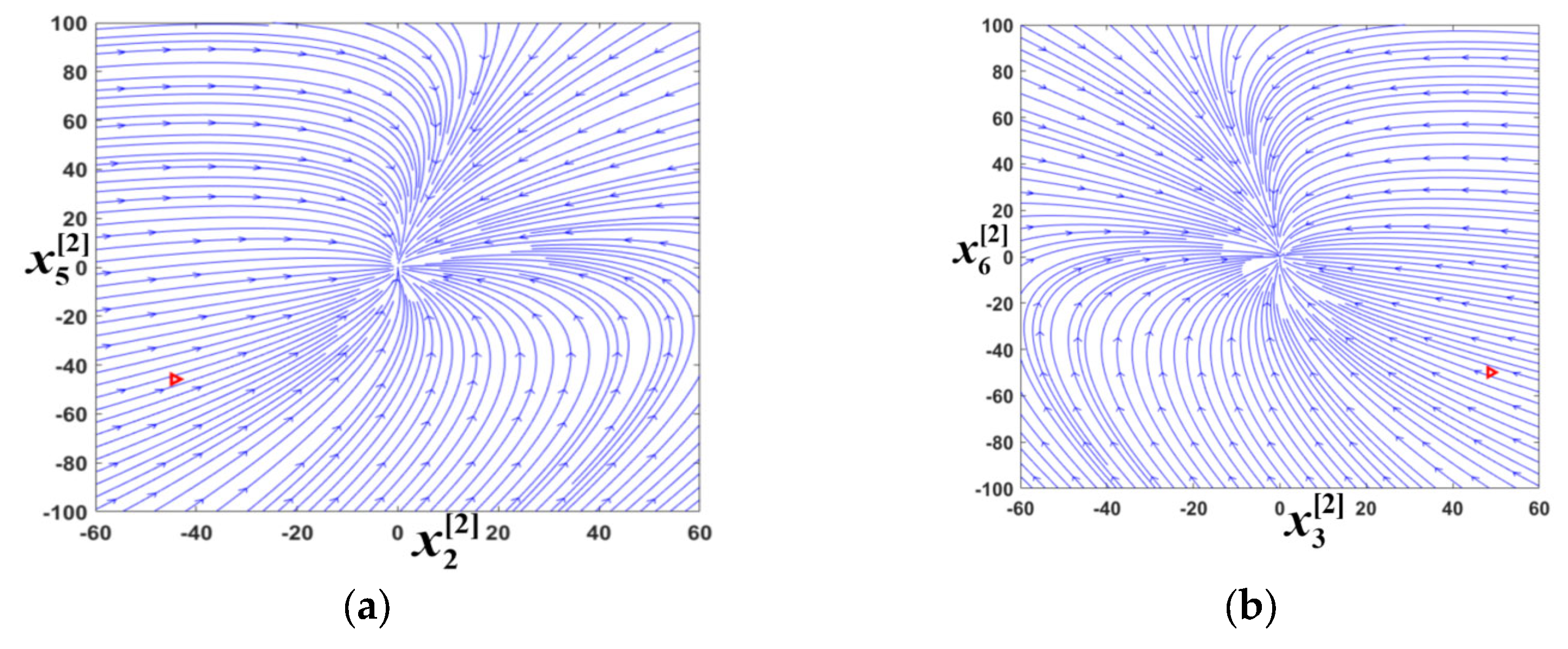
CASE III: Compared with the transient process of sudden voltage drop from 311 V to 31.1 V, the model parameters (voltage amplitude), the steady-state operation point, and the initial operation point significantly change when the grid voltage rises abruptly from 31.1 V to 311 V. The eigenvalues corresponding to the model are all real roots. The nonlinear decoupling method combines the two pairs of state variables with large coupling factors into coupled pairs. The remaining variables with limited coupling factors are kept as isolated variables. The phase diagrams of the coupling pairs and and are shown in Figure 13. The phase diagrams of these two coupling pairs are stable over a wide range, which prevents instability. The red triangles are still used to mark the initial positions of the corresponding state variables.
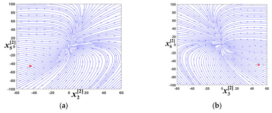
Figure 13.
Phase diagrams and the initial points for 31.1 V to 311 V. (a) Coupling pairs . (b) Coupling pairs .
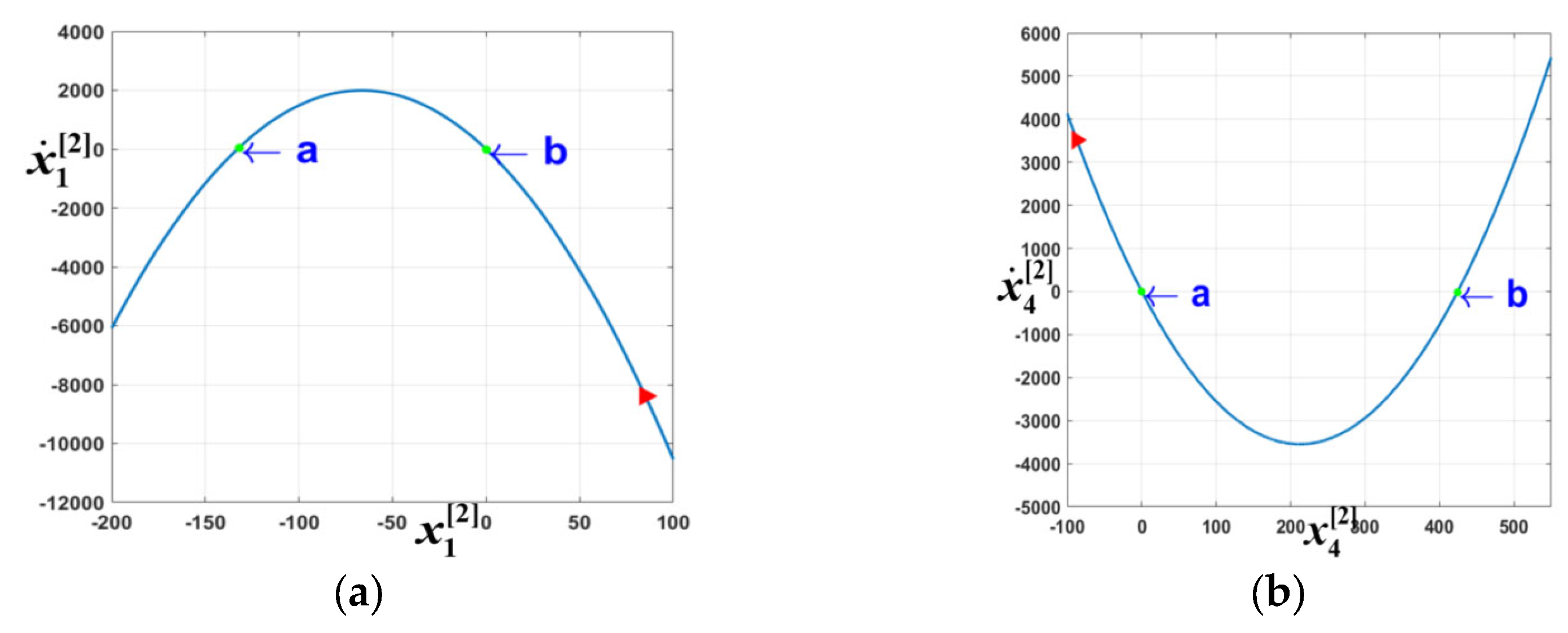
For isolated variables and , the diagram of can be calculated to view the ROA. As shown in Figure 14a, the curve intersects the axis at points a and b, and the red triangle marks the initial point. It can be easily proved that the ROA of is , which means that when the initial point is in the interval, the state variable returns to the stable operating point. According to Figure 14b, the ROA of the state variable is , and the initial point lies within the region. Hence, for a sudden voltage rise from 31.1 V to 311 V, all six variables are in stable regions, so the system is robust against large-signal instability.
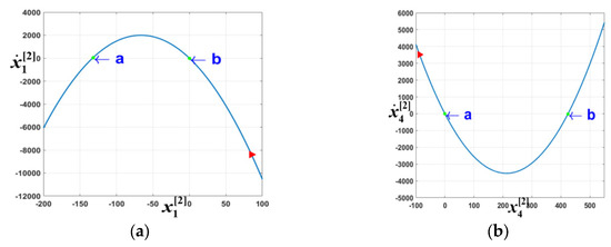
Figure 14.
ROA of the isolated variables for 31.1 V to 311 V. (a) Isolated variable . (b) Isolated variable .
A comparison of the above three cases indicates that large-signal instability occurs in the system when the grid voltage amplitude drops from 311 V to 31.1 V, but the system can maintain stability in the process of recovery from 31.1 V to 311 V. The cases also confirm that the large-signal stability of the nonlinear system needs to be analyzed by combining the initial and operation points.
4. Hardware-in-Loop Experiments
Corresponding HIL experiments are conducted to verify the effectiveness of the proposed method. The circuit is built in RTLAB, and the control strategy is implemented in TMS320F28335DSP. Figure 15 shows the experimental equipment and signal flow. The circuit parameters and the control parameters are the same as in Table 1.
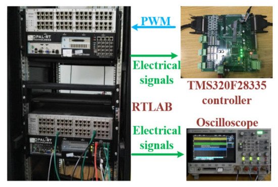
Figure 15.
HIL experimental equipment.
The experimental topology is consistent with Figure 8, where three VSCs are connected to the weak grid by line impedances. The sudden change in the grid voltage amplitude represents the large signal disturbance faced by the system.
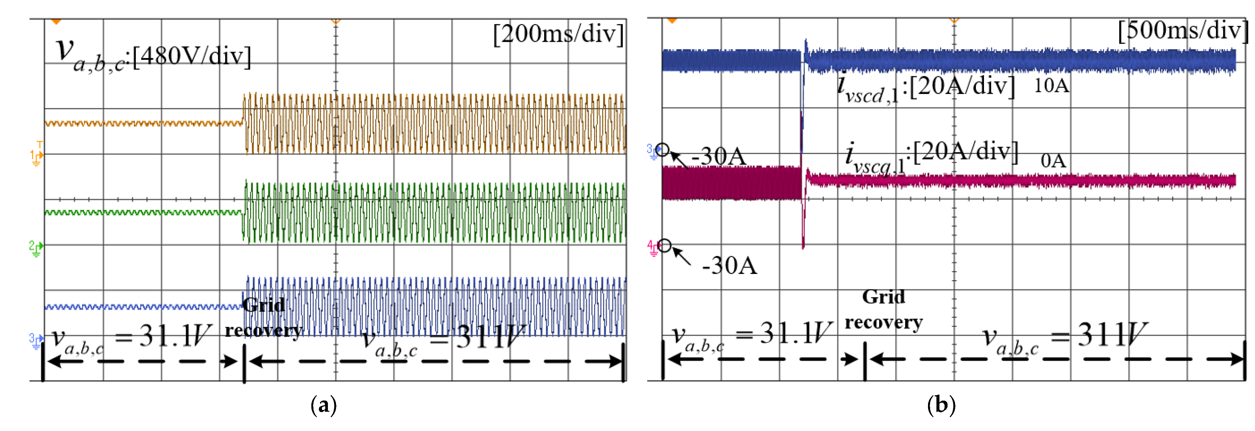
As the voltage amplitude drops from 311 V to 31.1 V, the corresponding waveforms are shown in Figure 16. Initially, the system is in the normal operation status. The grid voltage is 311 V, and the output current values of the three VSCs are consistent with the current reference values. The output phase angles of the VSCs are kept constant, which indicates that all the VSCs remain synchronized with the grid. When the grid voltage drops significantly to 0.1 pu, the output currents of VSC1 and VSC2 show a larger ripple. The phase angles deviate from the grid voltage and return around the initial values after experiencing a specific step. In contrast, the output current of VSC3 shows apparent oscillation, and its phase angle continues to increase until it exceeds the expression limit of the figure and cannot maintain stability, indicating that VSC3 has lost synchronization. Since the output current of VSCs has a significant fluctuation or oscillation and VSC3 has been out of step, the bus voltage cannot present the typical sinusoidal waveform, and the whole system is in a state of transient instability. Throughout the process, large changes in the bus voltage promote transient instability of the system, in which the VSC with a larger output current exhibits more prominent instability.
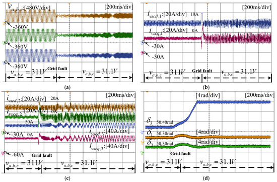
Figure 16.
Experimental results of VSCs when the voltage drops from 311 V to 31.1 V. (a) Grid voltage waveforms. (b) Active and reactive power waveforms of VSC1. (c) Active and reactive power waveforms of VSC2 and VSC3. (d) Phase angle of VSC1,2,3.
When the grid voltage is restored from 31.1 V to 311 V, the output currents of different VSCs and the phase angles are shown in Figure 17.
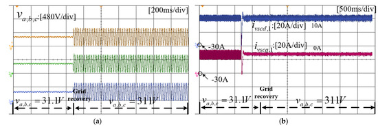

Figure 17.
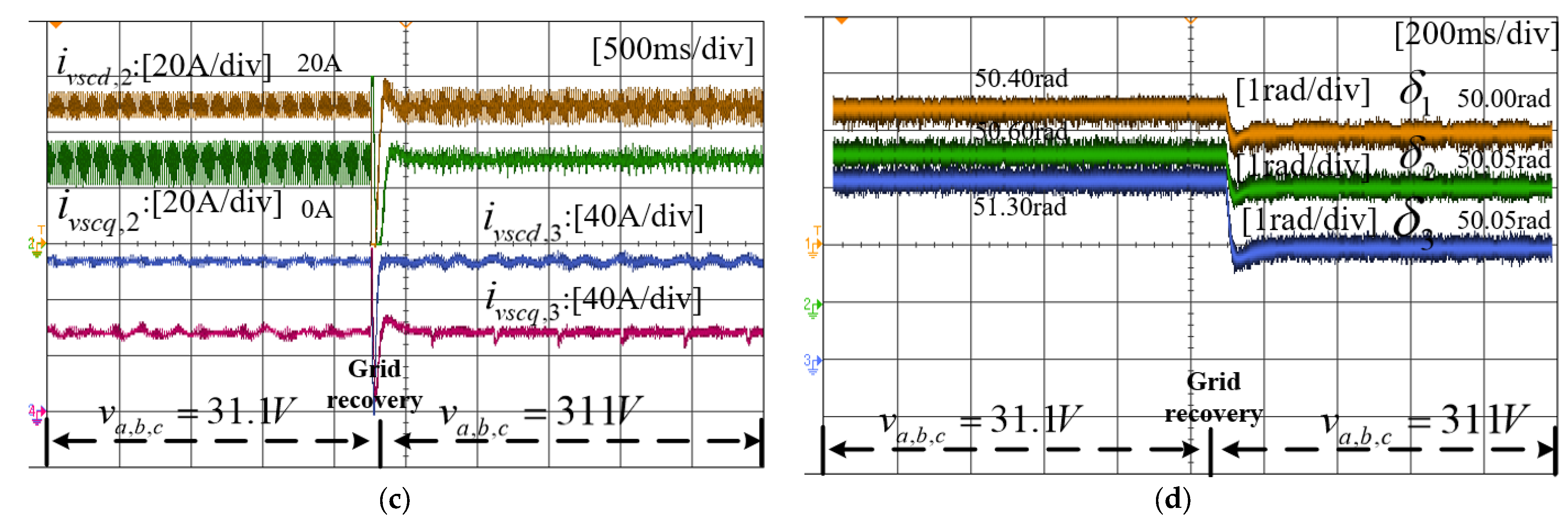
Experimental results of VSCs when voltage recovers from 31.1 V to 311 V. (a) Grid voltage waveforms. (b) Active and reactive power waveforms of VSC1. (c) Active and reactive power waveforms of VSC2 and VSC3. (d) Phase angle of VSC1,2,3.
According to Figure 17, the bus voltage recovers from 31.1 V to 311 V. Different from the process of voltage sag, Figure 17a shows that the voltage can maintain a stable sinusoidal waveform after recovery. Based on the output current waveforms of the VSCs, the output current can be maintained near the reference value before and after the voltage change. After the bus voltage recovers to the rated value, there is a specific reduction in the current ripple. In addition, the PLL tracking phase angles of the three VSCs exhibit a slight decrease, but all of them return to stability. The case represents the inverse process of the voltage drop, and the waveforms indicate that the system can remain stable under a wide range of fluctuations. Although the control and circuit parameters are unchanged, there are great differences in the transient stability caused by the voltage drop and voltage recovery. Thus, for a nonlinear system, the transient stability must be analyzed in combination with the specific operation points and the corresponding stability region.
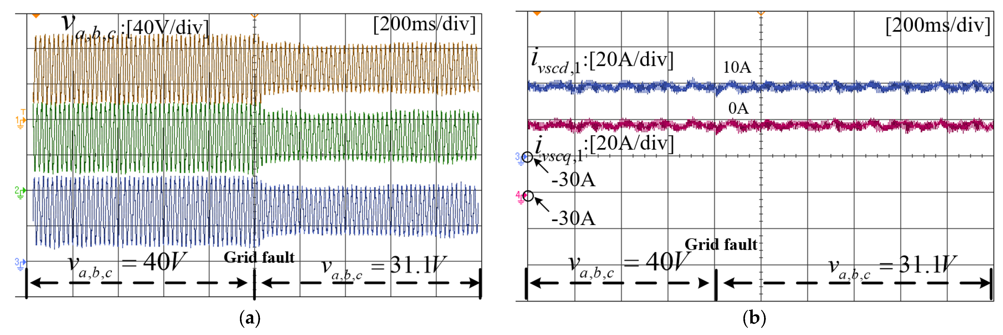
Similarly, when the grid voltage sags from 40 V to 31.1 V, the corresponding output current and phase angles are as shown in Figure 18, and the system can still maintain transient stability. During the drop in the voltage amplitude, the output current values remain equal to the reference values. Since the voltage amplitude does not change much, the transient performance of the output current change is relatively smooth. The tracking angles of VSC1 and VSC2 can be stabilized after a small oscillation, and the tracking angle of VSC3 can also be stabilized after a relatively large oscillation. The experimental results are consistent with the theoretical analysis, indicating that the system can maintain transient stability when the initial operating point lies within the stable region.
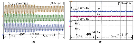
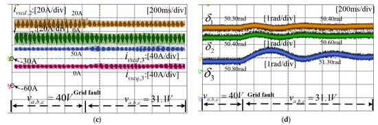
Figure 18.
Experimental results of VSCs when the voltage drops from 40 V to 31.1 V. (a) Grid voltage waveforms. (b) Active and reactive power waveforms of VSC1. (c) Active and reactive power waveforms of VSC2 and VSC3. (d) Phase angle of VSC1,2,3.
5. Conclusions
In this paper, the CFND method is proposed to investigate the transient stability of the multi-VSC parallel system. The CFND method evaluates the coupling degree between different state variables according to coupling factors and decouples the high-order model into several first-order and second-order modes. Directly using a full-order model analysis for multi-VSC grid-connected systems can introduce a significant computational burden. From the perspective of practical engineering applications, it is necessary to perform reasonable reduction and simplification for the VSC model. Thus, the reduced-order large-signal model and truncated model of the single-VSC grid-connected system are derived, and the effectiveness of the reduced-order model is verified through simulation waveforms and ROA partitioning. Subsequently, a reduced-order model of the multi-VSC grid-connected system is obtained through circuit equivalence. Taking the system with three VSCs as an example, the proposed CFND method is used to analyze typical operating conditions of the system, and the conclusions of transient stability analysis are verified using the HIL experiments.
Theoretical analysis and experimental results indicate that significant voltage fluctuations in the power grid can lead to transient instability in multi-VSC grid-connected systems. VSCs with higher active power output are more likely to experience transient instability. When the system voltage collapse is inevitable, control measures can be considered to make the voltage amplitude of the power grid drop multiple times in stages, which helps each VSC maintain synchronization with the power grid and helps the system to restore stable operation after the fault is cleared in the later stage.
Author Contributions
Methodology, Y.L. and Y.X.; Validation, J.M.; Writing—review & editing, Y.P. All authors have read and agreed to the published version of the manuscript.
Funding
This work was supported in part by the National Key R&D Program of China under Grant 2021YFB2401303, in part by the National Natural Science Foundation of China under Grant 52007162, and in part by the Key R&D Program of Zhejiang Province under Grant 2022C01161.
Data Availability Statement
No new data were created.
Conflicts of Interest
The authors declare no conflict of interest.
References
- He, X.; Geng, H.; Li, R.; Pal, B.C. Transient Stability Analysis and Enhancement of Renewable Energy Conversion System During LVRT. IEEE Trans. Sustain. Energy 2010, 11, 1612–1623. [Google Scholar] [CrossRef]
- Zhao, J.; Huang, M.; Yan, H.; Tse, C.K.; Zha, X. Nonlinear and Transient Stability Analysis of Phase-Locked Loops in Grid-Connected Converters. IEEE Trans. Power Electron. 2021, 36, 1018–1029. [Google Scholar] [CrossRef]
- Zhao, F.; Shuai, Z.; Huang, W.; Shen, Y.; Shen, Z.J.; Shen, C. A Unified Model of Voltage-Controlled Inverter for Transient Angle Stability Analysis. IEEE Trans. Power Deliv. 2022, 37, 2275–2288. [Google Scholar] [CrossRef]
- Taul, M.G.; Wang, X.; Davari, P.; Blaabjerg, F. An Overview of Assessment Methods for Synchronization Stability of Grid-Connected Converters Under Severe Symmetrical Grid Faults. IEEE Trans. Power Electron. 2019, 34, 9655–9670. [Google Scholar] [CrossRef]
- Ma, S.; Geng, H.; Liu, L.; Yang, G.; Pal, B.C. Grid-Synchronization Stability Improvement of Large Scale Wind Farm During Severe Grid Fault. IEEE Trans. Power Syst. 2018, 33, 216–226. [Google Scholar] [CrossRef]
- Zhou, Y.; Xin, H.; Wu, D.; Wang, G.; Yuan, H.; Ju, P. Small-Signal Stability Boundary of Heterogeneous Multi-Converter Power Systems Dominated by the Phase-Locked Loops’ Dynamics. IEEE Trans. Energy Convers. 2022, 37, 2874–2888. [Google Scholar] [CrossRef]
- Li, Y.; Fan, L. Stability Analysis of Two Parallel Converters with Voltage–Current Droop Control. IEEE Trans. Power Deliv. 2017, 32, 2389–2397. [Google Scholar] [CrossRef]
- Yang, P.; Yu, M.; Wu, Q.; Hatziargyriou, N.; Xia, Y.; Wei, W. Decentralized Bidirectional Voltage Supporting Control for Multi-Mode Hybrid AC/DC Microgrid. IEEE Trans. Smart Grid 2020, 11, 2615–2626. [Google Scholar] [CrossRef]
- Guo, J.; Meng, Z.; Chen, Y.; Wu, W.; Liao, S.; Xie, Z.; Guerrero, J.M. Harmonic Transfer-Function-Based αβ-Frame SISO Impedance Modeling of Droop Inverters-Based Islanded Microgrid with Unbalanced Loads. IEEE Trans. Ind. Electron. 2023, 70, 452–464. [Google Scholar] [CrossRef]
- Gless, G.E. Direct method of Lyapunov applied to transient power system stability. IEEE Trans. Power Appar. Syst. 1966, PAS-85, 159–168. [Google Scholar] [CrossRef]
- Tian, T.; Kestelyn, X.; Thomas, O.; Amano, H.; Messina, A.R. An Accurate Third-Order Normal Form Approximation for Power System Nonlinear Analysis. IEEE Trans. Power Syst. 2018, 33, 2128–2139. [Google Scholar] [CrossRef]
- Wang, Z.Q.; Huang, Q.; Zhang, C.H. An Improved Poincaré-like Carleman Linearization Approach for Power System Nonlinear Analysis. J. Electr. Eng. Technol. 2013, 8, 271–281. [Google Scholar] [CrossRef]
- He, X.; Geng, H.; Ma, S. Transient stability analysis of grid-tied converters considering PLL’s nonlinearity. CPSS Trans. Power Electron. Appl. 2019, 4, 40–49. [Google Scholar] [CrossRef]
- Wu, H.; Wang, X. Design-Oriented Transient Stability Analysis of PLL-Synchronized Voltage-Source Converters. IEEE Trans. Power Electron. 2020, 35, 3573–3589. [Google Scholar] [CrossRef]
- Tang, Y.; Tian, Z.; Zha, X.; Li, X.; Huang, M.; Sun, J. An Improved Equal Area Criterion for Transient Stability Analysis of Converter-Based Microgrid Considering Nonlinear Damping Effect. IEEE Trans. Power Electron. 2022, 37, 11272–11284. [Google Scholar] [CrossRef]
- Wang, X.; Taul, M.G.; Wu, H.; Liao, Y.; Blaabjerg, F.; Harnefors, L. Grid-Synchronization Stability of Converter-Based Resources—An Overview. IEEE Open J. Ind. Appl. 2020, 1, 115–134. [Google Scholar] [CrossRef]
- Cheng, H.; Shuai, Z.; Shen, C.; Liu, X.; Li, Z.; Shen, Z.J. Transient Angle Stability of Paralleled Synchronous and Virtual Synchronous Generators in Islanded Microgrids. IEEE Trans. Power Electron. 2020, 35, 8751–8765. [Google Scholar] [CrossRef]
- Chen, S.; Yao, J.; Liu, Y.; Pei, J.; Huang, S.; Chen, Z. Coupling Mechanism Analysis and Transient Stability Assessment for Multiparalleled Wind Farms During LVRT. IEEE Trans. Sustain. Energy 2021, 12, 2132–2145. [Google Scholar] [CrossRef]
- Pal, D.; Panigrahi, B.K. Reduced-Order Modeling and Transient Synchronization Stability Analysis of Multiple Heterogeneous Grid-Tied Inverters. IEEE Trans. Power Deliv. 2022, 38, 1074–1085. [Google Scholar] [CrossRef]
- Amano, H.; Yokoyama, A. Rotor Angle Stability Analysis Using Normal form Method with High Penetrations of Renewable Energy Sources-Energy Index for Multi-Swing Stability. In Proceedings of the 2018 Power Systems Computation Conference (PSCC), Dublin, Ireland, 11–15 June 2018; pp. 1–6. [Google Scholar]
- Wang, B.; Sun, K.; Kang, W. Nonlinear Modal Decoupling of Multi-Oscillator Systems with Applications to Power Systems. IEEE Access 2018, 6, 9201–9217. [Google Scholar] [CrossRef]
- Xia, Y.; Lv, Z.; Wei, W.; He, H. Large-Signal Stability Analysis and Control for Small-Scale AC Microgrids With Single Storage. IEEE J. Emerg. Sel. Top. Power Electron. 2022, 10, 4809–4820. [Google Scholar] [CrossRef]


Disclaimer/Publisher’s Note: The statements, opinions and data contained in all publications are solely those of the individual author(s) and contributor(s) and not of MDPI and/or the editor(s). MDPI and/or the editor(s) disclaim responsibility for any injury to people or property resulting from any ideas, methods, instructions or products referred to in the content. |
© 2023 by the authors. Licensee MDPI, Basel, Switzerland. This article is an open access article distributed under the terms and conditions of the Creative Commons Attribution (CC BY) license (https://creativecommons.org/licenses/by/4.0/).