Abstract
As the demand for power supply increases, the investment in the power transmission system constantly increases. An accurate economic evaluation of the power transmission system is essential for future investment decisions and management. Applying a single method in economic evaluation leads to excessive subjective consciousness and unreasonable weight allocation. The Euclidean distance in the traditional TOPSIS method only partially works on the condition that the criteria are linearly correlated. To solve these problems, an economic evaluation method based on improved TOPSIS and BWM-anti-entropy weight is proposed. For the assignment of weights, the method retains the advantages of subjective and objective weighting methods based on the Nash equilibrium, breaks through the limitation of utilizing a single method, which contributes to one-sided results, and enhances the scientific rigor and rationality of the comprehensive weighting process. Furthermore, based on comprehensive weights, the method improves the TOPSIS by introducing the Mahalanobis distance and Pearson correlation coefficients, which can eliminate the influence of linear correlation. Finally, ten 500 kV transmission and transformation projects are analyzed and ranked to verify the method’s feasibility. Empirical analysis shows that the method can effectively evaluate the economic benefits of the power transmission system.
1. Introduction
Energy and environmental problems are becoming increasingly prominent, and electrical energy is an indispensable secondary energy source in society. As the industry has progressed in recent years, electricity consumption has steadily increased, resulting in elevated demands for power supply reliability and safety. The power transmission system is an integral part of the electric power system—which includes transmission lines, substations, and related equipment—influencing the quality of power supply and economic and social development. The power transmission system has a significant investment scale and a long construction period [1]. Therefore, the economics of power system projects in terms of profitability, liabilities, etc. need to be quantified and comprehensively evaluated for managerial decision-making and planning.
A comprehensive evaluation uses scientific, feasible methods to evaluate and analyze all aspects of the evaluation: object behavior, multi-indicator, and multi-level. Some studies have concluded that the economic evaluation of the power transmission system focuses on cost and benefit. Based on the cost–benefit analysis, the scores for multiple power transmission systems can be calculated and ranked [2]. According to the characteristics of the power system project, the economic evaluation of the project is divided into two parts: financial analysis and economic cost-effectiveness analysis [3]. Subsequently, increasing numbers of people are researching and improving the evaluation system and criteria for power transmission systems. A two-tier indicator system for investment effectiveness evaluation was established, considering both unit- and macro-investment effectiveness [4]. To combine the metrics of investment effectiveness and investment efficiency, the criteria of comprehensive economic evaluation can be categorized into basic, modified, and appraisal criteria [5]. Existing research provides an important reference for the economic evaluation of the power system in this paper. This paper considers the three perspectives of time, value, and efficiency to establish a comprehensive evaluation system from the three aspects of profitability, solvency, and development capability.
Regarding models and methods for the economic evaluation of power transmission systems, many relevant research studies already exist in the field of MCDA. Multi-criteria decision analysis (MCDA) is a complex field of decision-making disciplines for problems with multiple criteria and multiple choices that can be used for economic evaluation [6]. The core methods and techniques are WSM, TOPSIS, AHP, PROMETHEE, ELECTRE, COMET, and SIMUS [7]. The weighted sum method (WSM) is the most commonly used [8] for assessment and decision-making in a single dimension. The analytical hierarchy process (AHP) uses a hierarchical structure to decompose a complex problem to evaluate the objectives at the top of the structure [9]. The ELECTRE method can be iterated to provide a ranking of alternatives based on consistency and thresholds [10]. The combined approaches are also proposed, and some previous research conducted a comprehensive analysis by establishing a fuzzy synthetic evaluation model using the hierarchical analysis method [11]. Pareto optimal function and merit criterion methods are also employed to enhance project comparison and decision-making [12,13]. In the study [14], which optimizes the fuzzy synthetic evaluation model, a hierarchy evaluation model for fuzzy analysis is built based on a novel comprehensive fuzzy evaluation operator. However, this model relies too much on subjectivity. A combination of the entropy weighting method and gray correlation analysis is employed to address the challenges posed by incomplete information and the subjective nature of weights. Then, the improved gray correlation analysis method is used to arrive at the optimal solution [15]. Based on the content and characteristics of specific projects in the power system, this paper proposes the improved TOPSIS method. TOPSIS is a multi-criteria decision analysis method that can be used to evaluate objects across multiple areas with satisfactory results [16]. The original TOPSIS method is likely to lead to the problem of rank reversal when changing the number of items to be evaluated [17], and the TOPSIS method can be improved by introducing the absolute ideal solution [18,19]. The absolute ideal solution provides initial support for our improvements to TOPSIS. We find that indicators are often correlated, and that correlation leads to partial failure of the Euclidean distance in traditional TOPSIS [20,21]. Although many methods and software have been applied to build evaluation systems and accurately evaluate the economics of power transmission systems, few weights can balance subjective experience and objective data.
Previous studies have often used single-dimension weights to evaluate economics, with some articles considering only subjective weights [22,23] (AHP, BWM), and some articles considering only objective weights [24,25](EWM, PCA). Combinations of subjective and objective methods are also often used in the field of evaluation [26,27]. The construction of the coupling coordination model is dependent on the coordination of weights estimated by AHP and EWM methods [28]. In the paper [29], a novel hybrid multi-criteria decision-making (MCDM) approach is devised for offshore wind turbine selection by assignment of weights using ANP and EWM. Given the limitations of assigning weights to a single dimension, we propose the BWM-anti-entropy weight method in this paper, which utilizes a game theory model to balance subjective and objective weights. Game theory models can ultimately result in more efficiently comprehensive weights [30].
In summary, based on comprehensive weights and absolute ideal solutions, the TOPSIS method can be improved using the Mahalanobis distance and Pearson’s correlation coefficient. This final improved TOPSIS method is more scientific and logical.
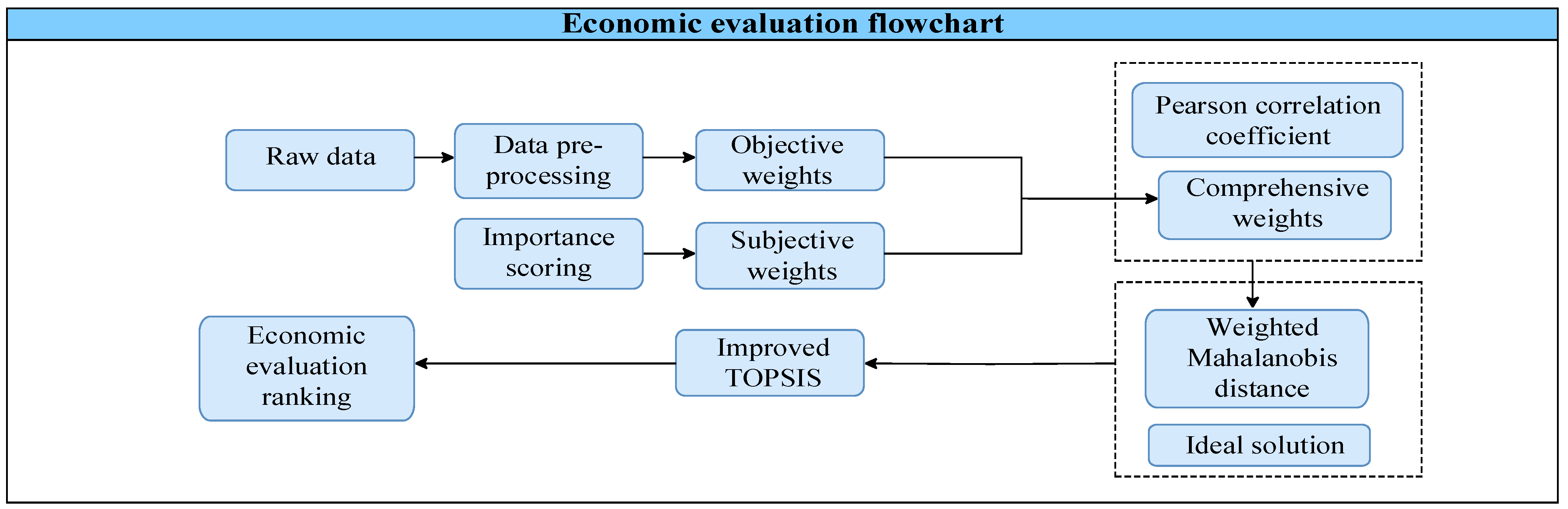
The key processes of the improved TOPSIS method are illustrated in Figure 1.
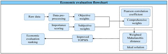
Figure 1.
Economic evaluation flowchart.
Other contents are organized as follows: The economic evaluation system of power transmission systems is constructed in Section 2, focusing on three aspects and determining the specific evaluation criteria. In Section 3, the subjective weights and objective weights are calculated, then an integrated weighting model is established by applying the game theory. Section 4 outlines the deficiencies of the traditional TOPSIS method and introduces the improved TOPSIS method utilizing the Mahalanobis distance and Pearson coefficient. In Section 5, the comparison analysis is carried out on the specific data of 500 kV transmission and transformation projects to acquire the evaluation results for the proposed criterion system, model, and improved method.
2. The System of Criteria for Economic Evaluation
The comprehensive evaluation of economic efficiency in this paper is based on the financial evaluation criterion system.
According to the characteristics of the power transmission system and the theory of financial evaluation criteria, this paper establishes the evaluation system from three perspectives: financial profitability, financial solvency, and financial development capability [31]. The evaluation of comprehensive economic efficiency is carried out mainly from the perspectives of time, value, and efficiency [32,33], and these three perspectives are substantially equivalent, which means that many of the criteria are consistent at their core.
Under each perspective, the appropriate criteria should be selected for the description. The information on different criteria is used for the economic evaluation of the power transmission system. The specific criteria system is shown in Table 1.

Table 1.
Economic evaluation criteria system.
- 1.
- Return on Investment (ROI)
ROI is a performance assessment used to evaluate the efficiency of an investment or to compare the efficiency of many different investments. ROI directly measures the amount of return on a particular investment relative to the cost of the investment. The ratio and profitability of the power transmission system have a significant positive correlation. The calculation formula is defined as shown in Equation (1) [34]:
where is Annual net income, is total investment (including construction investment and working capital).
- 2.
- Net Present Value (NPV)
Net present value (NPV) is the equivalent present value of the net cash flow for each year of the power transmission system life cycle discounted at a given discount rate, calculated as shown in Equation (2) [34]:
where is cash inflows by year, is cash outflows by year, is the whole life cycle of the power transmission system, including the construction period and operation period.
- 3.
- Payback Period (Pt)
The payback period is the time required to recover the entire investment in a power transmission system in terms of its net income, usually in years. The payback period ends when a transmission system’s net benefits equal the total initial investment. This number of years to recover the investment. This paper uses a static payback period without considering the time value. The formula is expressed in Equation (3) [34]:
where is net cash flow.
- 4.
- Internal Rate of Return (IRR)
The internal rate of return (IRR) is the discount rate when the cumulative present value of the net cash flow over the life cycle of the power transmission system is zero. Internal rate of return (IRR) is the main dynamic evaluation criterion used to examine the profitability of the power transmission system, reflecting the profitability of the whole investment during its life. This is given by Equation (4) [34]:
where is net cash flow, is the whole life cycle of the power transmission system, including the construction period and operation period.
- 5.
- Asset Liability Ratio (ALR)
Asset liability ratio refers to the percentage of total liabilities to total assets, reflecting the degree of financial risk and the liabilities of power transmission systems. This is given by Equation (4) [34]:
where is total liabilities, is total assets.
- 6.
- Current Ratio (CR)
The current ratio reflects the ability of the power transmission system to repay the current outstanding liabilities each year. It is an essential indicator of the short-term solvency of the power transmission system. The calculation formula [34] is:
- 7.
- Profit Growth Rate
The profit growth rate refers to the growth rate of the net profit of the power transmission system in the current period compared with the net profit in the previous period, and the larger the indicator’s value, the stronger the profitability [34].
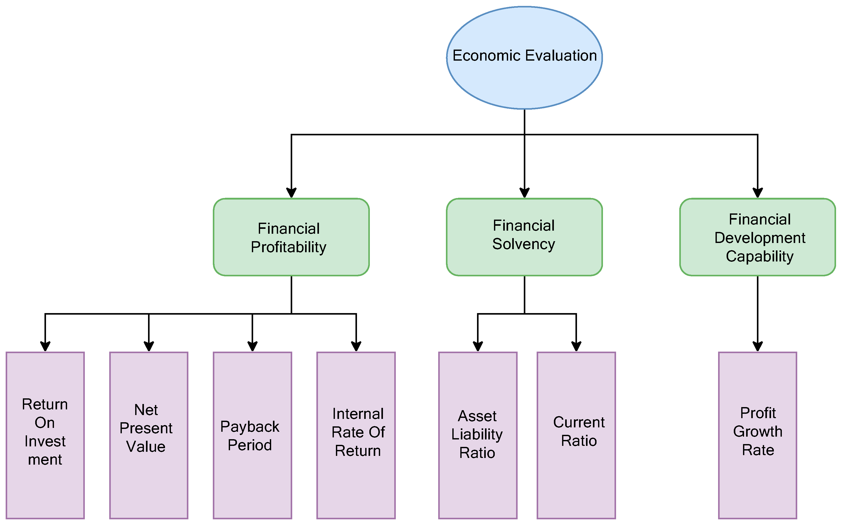
The economic evaluation criteria system is shown in Figure 2.
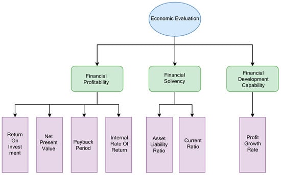
Figure 2.
Economic evaluation criteria system.
3. Comprehensive Weighting Solution Model
3.1. Subjective Weight Solving Based on the BWM Method
The BWM is proposed to determine the subjective weights of the criteria [35]. In the past, the most common method was the AHP method, which compares any two indicators with each other to determine the evaluation matrix of the indicators. This requires comparisons to determine the data [36]. Compared to the AHP method, the BWM is less cumbersome and data-intensive, reducing errors caused by confused thinking. The BWM makes it easier to pass the consistency test, making the results more reliable [37].
The BWM (best-worst method) is frequently used in multi-criteria decision-making [38]. Experts select the most important and least important criteria based on experience and practical engineering needs, then compare the best criterion with the rest of the criteria, and then compare the worst criterion with the rest. An integer value of 1–9 reflects the relative significance among the indicators. The specific procedures are as follows:
STEP 1: Identify the influencing factors of multi-criteria evaluation issues and establish a set of criteria based on the influencing factors of different aspects.
STEP 2: Identify the most important criterion and the least important criterion.
STEP 3: Compare the best, worst, and other criteria separately to create two vectors that characterize relative preferences. , .
For the criteria system of the power transmission system, two scoring tables are established, as shown in Table 2 and Table 3.
Table 2.
Scoring the relative importance of the best criterion.
Table 3.
Scoring the relative importance of the worst criterion.
STEP 4: Build a mathematical subjecting model and find the best solution to obtain the objective optimal weights. The mathematical planning [35] is as follows:
where is the weight of , is the weight of the base vector , i.e., the actual weight of the criteria, is the weight of , is the value of the importance of relative to , is the value of the importance of relative to .
STEP 5: Use the following formula [35] to calculate ; = 0 represents complete consistency. The closer it is to 0, the better the consistency.
where the obtained by Equation (8) is called , is a constant.
3.2. Objective Weight Solving Based on the Anti-Entropy Method
The entropy value is frequently mentioned when seeking objective weights in multi-criteria decision-making models. Both entropy and anti-entropy methods share a key feature: they solve for objective weights [39]. These two approaches both believe that the volatility in the data of a criterion is positively correlated with its weight. If this criterion is approximately equal for each power transmission system, then the weight corresponding to this criterion should be small. The essence of information entropy is the expected value of the amount of information.
The entropy method has been improved to become the anti-entropy method. It has the characteristic that the stronger the volatility of the criterion, the smaller the entropy value and the larger the weight coefficient [40]. The specific procedure of the anti-entropy weight method is as follows:
STEP 1: The initial matrix must be created and normalized for a comprehensive evaluation model with subjects of evaluation and criteria.
The matrix with subjects and criteria is :
The initial matrix is normalized using the vector normalization method:
The matrix is normalized to eliminate the effect of the physical dimensions, and the normalized matrix is obtained.
STEP 2: Calculate the share of the subject under the criterion and consider it as the probability used in the relative entropy calculation.
where is considered as the probability of the subject under the criterion.
The anti-entropy is calculated in Equation (14) [25]:
For each criterion, its objective weight is calculated in Equation (15) [25]:
where is the anti-entropy weight of the criterion .
3.3. Coordination of Subjective and Objective Weights Based on Game Theory
Subjective weighting methods such as BWM depend heavily on experts’ personal experiences and ideas and have some limitations. The objective weighting method is based on the data but may deviate from the actual situation. The BWM-anti-entropy weighting method is combinatorial. It is based on game theory’s ideology and considers subjective and objective weights. The BWM-anti-entropy weighting method regroups the two sets of weights into a more scientific and reasonable combined weighting.
The comprehensive weighting method, which averages the two sets of weights, is unreasonable and does not effectively eliminate the shortcomings of the two weighting methods. Using game theory, this method takes Nash equilibrium as the optimum goal, coordinates the two sets of weights to find a balance, and makes the discrepancy between the final comprehensive weights and the two original sets of weights as minimal as possible to derive a set of more scientific comprehensive weights.
STEP 1: Obtain the weights of each criterion by subjective and objective methods, respectively. A basic set of weights is constructed based on this. The arbitrary linear combination of these vectors constructs the set of comprehensive weights.
where is the subjective weight, is the objective weight, and is the linear coefficient that needs to be optimized using the model.
STEP 2: Optimize using a game-theoretic model that minimizes the deviation from each . The following policy response model [41] is used:
STEP 3: Utilize the differential property to convert the matrix constraints for the optimal solution:
Solve the equation normalization process:
Optimization problems such as comprehensive weights can also be solved using Lagrange multipliers. To make the comprehensive weight closer to both objective and subjective weights, the function is established [42] as follows:
where is the optimal combination weight, is the subjective weight, and is the objective weight.
The equation solved by the Lagrange multiplier is shown as Equation (22) [42].
4. An Improved TOPSIS
4.1. A Solution to the TOPSIS Reverse Order Problem
The TOPSIS method constructs the multi-indicator problem’s ideal and negative ideal solutions. It ranks the feasible solutions based on the evaluation criterion of the distance approximate to the absolutely ideal solution and away from the absolutely negative ideal solution.
In the traditional TOPSIS method, the reversal of order is a very prone problem for sorting multiple solutions. The root cause of the reverse order is the change in the ideal and negative ideal solutions of the decision problem after the addition of a new decision solution, which leads to a change in the evaluation criteria and, thus, to a change in the order of the superiority of the solutions [43].
If this relative ideal solution can be abandoned and absolute ideal and negative ideal solutions are defined, order reversal will not occur. More precisely, no solution is better than the absolute ideal solution or worse than the negative ideal solution in a valid decision region. Based on this concept, we define the absolutely positive ideal solution for the benefit-based criteria as follows: . Likewise, we define the absolutely negative ideal solution as follows: .
4.2. Improved TOPSIS Based on Mahalanobis Distance
The Mahalanobis distance is irrelevant to the measurement scale and is not influenced by the magnitude. The covariance between criteria is added to measure the association between them. By doing so, the effect of correlation between the criteria on the distance measurement is to some extent reduced. The fundamentals of TOPSIS and the Mahalanobis distance are detailed in Appendix A.
The equation [44] for the Mahalanobis distance of and :
where is the covariance matrix.
The Mahalanobis distance only considers the covariance between the criteria. However, it solves the problem of different magnitudes between criteria and overcomes the problem of linear correlation of the criteria. However, the inverse covariance matrix only characterizes the fluctuation of the criteria compared to the mean, which may overestimate the influence between criteria, leading to inconsistent results. The Mahalanobis distance can be improved. Firstly, it would be better to use the Pearson correlation coefficient in comparison to the covariance [45]. This is because the magnitude of the criterion influences the covariance and avoids the significant differences in values that lead to poor correlation. The Pearson correlation coefficient is limited to [−1, 1], which is more reasonable. Secondly, the Mahalanobis distance should be added to the comprehensive weights obtained in the previous section to calculate the distance more scientifically. In summary, the improved expression of the weighted Mahalanobis distance is as follows:
where is the Pearson correlation coefficient matrix, and are the comprehensive weights.
The steps of the improved TOPSIS comprehensive evaluation model are shown below:
STEP 1: Calculate the Pearson correlation coefficient between each criterion.
STEP 2: Conduct a normalization of different types of metrics (benefit-based, cost-based, intermediate value)
For benefit-based criteria [44]:
For cost-based criteria [44]:
For intermediate-value criteria:
STEP 3: Calculate the distance from the subject to the absolutely positive ideal subject and the distance to the absolutely negative ideal subject , respectively, with Equations (29) and (30).
where is the vector of normalized data on the criteria for the subject, and is the Pearson correlation coefficient matrix.
STEP 4: Calculate the relative closeness. A large relative closeness value responds to an economically efficient subject [44].
5. Example Analysis and Comparison
Transmission and transformation projects are the basic projects for the realization of the transmission system, which is responsible for the construction and maintenance of the lines and facilities required for the transmission system. This section analyzes data related to ten 500 kV transmission and transformation projects. These projects are comprehensively evaluated using the improved TOPSIS and BWM-anti-entropy weight method. First, the subjective and objective weights are sought, and then the comprehensive weights are obtained by applying game theory. Finally, a comprehensive evaluation of the ten projects is carried out based on the calculated comprehensive weights and the improved TOPSIS method.
5.1. Weighting Solution
5.1.1. Subjective Weights
The preferences of each criterion concerning the best and worst criterion are calculated in the order of 1 to 9, according to the order of comparing the best criterion with the other indicators and the other indicators with the worst criterion.
Select the Best: Return on Investment
Select the Worst: Profit Growth Rate
The specific scores are detailed in Table 4.
Table 4.
Scoring the relative importance of the best and worst criteria.
The results of the consistency test calculated according to the formula are:
; so, the pairwise comparison consistency level is acceptable.
After solving the mathematical planning, the optimal weights of BWM are shown in Table 5. The percentages and comparisons for the criteria are shown in Figure 3.
Table 5.
Subjective weights.
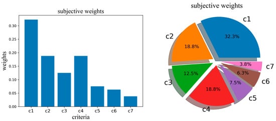
Figure 3.
Subjective weights.
5.1.2. Objective Weights
In this paper, anti-entropy weighting is applied for the objective weighting solution. This method derives its principle from the coefficient of variation and entropy weights.
Seven criteria are normalized for ten 500 kV transmission projects. The normalized matrix is detailed in Table 6.
Table 6.
Vector normalization.
The anti-entropy and weights of each criterion obtained according to the relevant formula of the anti-entropy weighting method are listed in Table 7.
Table 7.
Anti-entropy and subjective weights.
The weights and anti-entropy derived from the anti-entropy weights method can be seen: Net Present Value and Return On Investment have higher volatility and thus higher anti-entropy and weights. The data of other criteria do not change too much, and the weights are within a reasonable range.
5.1.3. Optimal Comprehensive Weights
Neither subjective nor objective weights can fully cover the information provided by the criteria. This section calculates the comprehensive weights using the Nash equilibrium and Lagrange multiplier methods.
According to the game model given by the Nash equilibrium in this paper, the coefficients of the combination of subjective and objective weights, which satisfy the Nash equilibrium, are 0.2241 = 0.7758. The combined Nash weights obtained by combining the two weights by the coefficients: . The percentages and comparisons for the criteria are detailed in Figure 4.
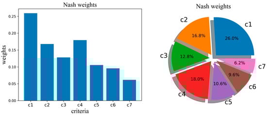
Figure 4.
Nash weights.
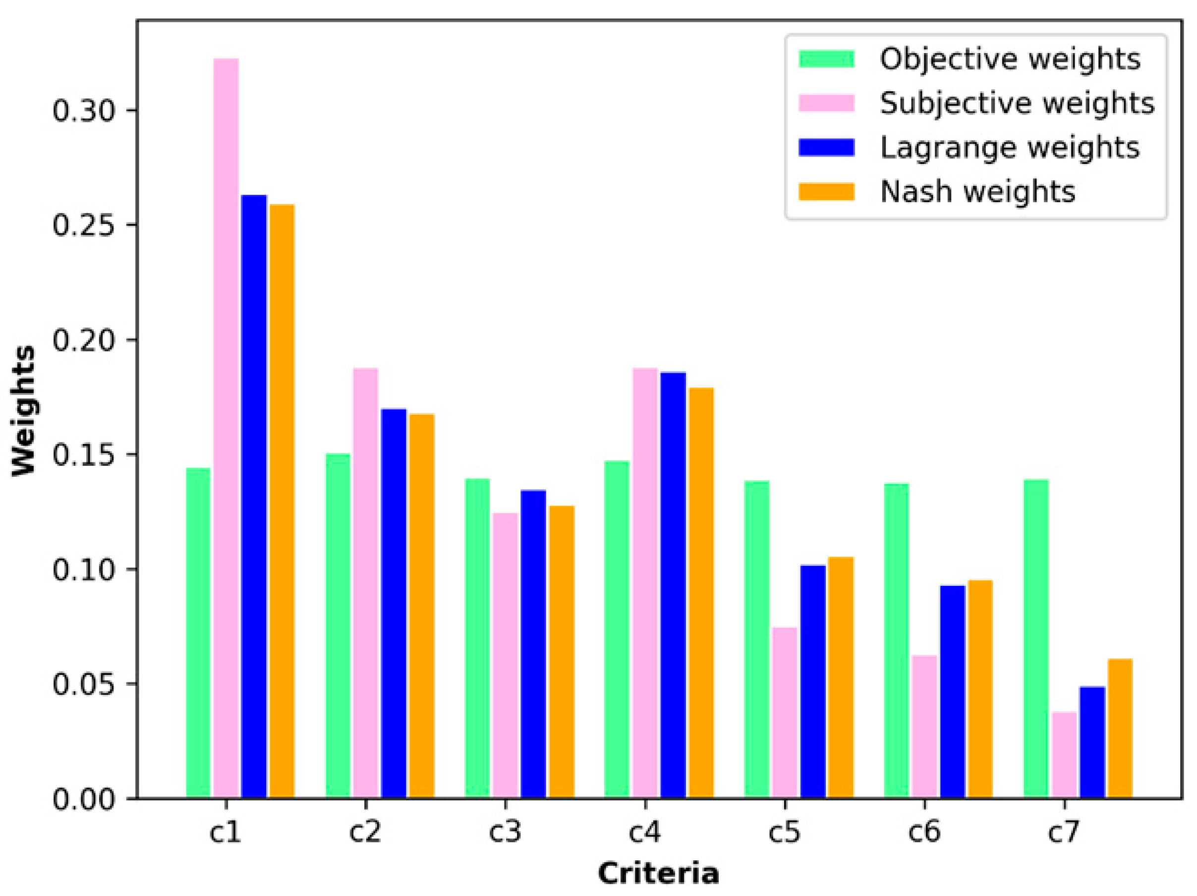
The Lagrange multiplier method can also solve the problem of finding the extrema under a set of constraints. Solving the objective function with the Lagrange multiplier method yields the optimal combination of weights: . A comparison of the two sets of basic weights (subjective, objective) and the two sets of combined weights (Nash, Lagrange) is shown in Figure 5.
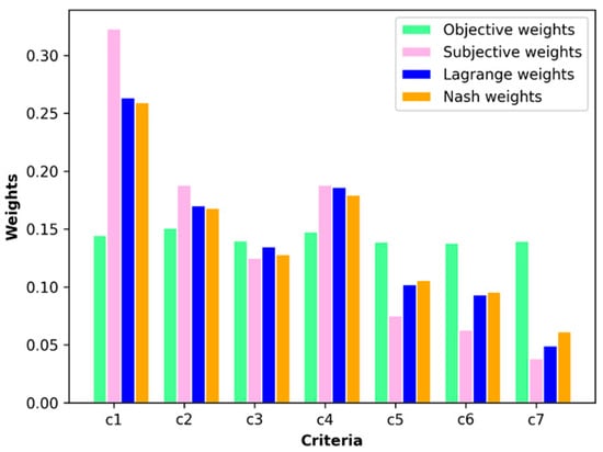
Figure 5.
Comparison of different weighting methods.
This section solves the comprehensive weights in two separate approaches. Comparing the two combined weights, the Nash and Lagrange weights are very similar, and both are between the subjective weights and objective weights. In this paper, Nash weight is chosen as the comprehensive weight of BWM-anti-entropy.
5.2. An Improved TOPSIS Method to Calculate Score Evaluation
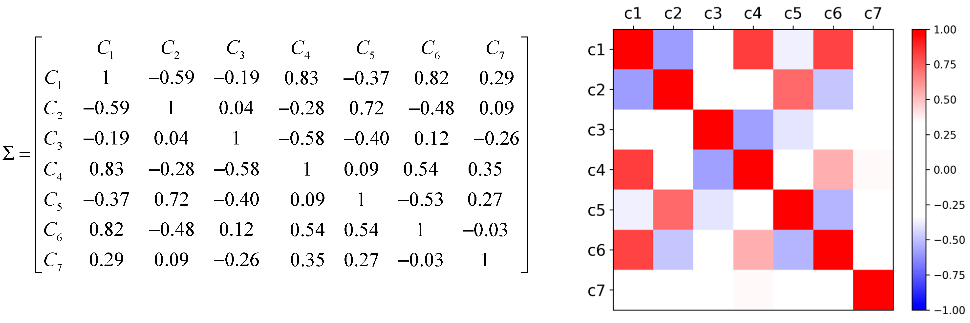
The Pearson correlation coefficient matrix between the seven criteria is shown in Figure 6.

Figure 6.
Pearson correlation coefficient matrix.
As can be seen from this Pearson correlation coefficient matrix, some of these criteria are strongly correlated. If we continue to use the Euclidean distance, it will lead to the failure of the Euclidean distance and will be unable to correctly assess the distance from the actual projects to the ideal projects. At the same time, using the inverse Pearson coefficient matrix as a substitute for the inverse covariance matrix will reduce the influence of the magnitude to a certain extent and more reasonably measure the degree of correlation between the criteria.
The data-processed results in advance by Max-Min normalization are detailed in Table 8.
Table 8.
Max-Min normalization.
The comprehensive weights and Pearson correlation coefficient matrices obtained from the Nash game model are used in TOPSIS to solve for the Mahalanobis distance.
The equation is used to find the Mahalanobis distance and the relative closeness of the evaluated solutions to the absolutely positive ideal projects and the negative ideal projects, and the evaluation projects are ranked according to the closeness. High relative closeness indicates that the project should be good. The Mahalanobis distance and closeness ranking are shown in Table 9.
Table 9.
Mahalanobis distance and closeness ranking.
After comparing the data with the final distance and closeness in Table 9, it can be seen that the relative closeness of is the highest. This is mainly because the two criteria with the highest weights, Return on Investment and Internal Rate of Return, are optimal. In contrast, for the cost-based criterion Asset Liability Ratio, is low. For , all four criteria characterizing profitability (c1~c4) are low, leading to poor evaluation results.
5.3. SIMUS and Traditional TOPSIS Solving
So far some of the more popular MCDM methods are AHP, TOPSIS, SPOTIS, COMET, SIMUS, etc. The SPOTIS method no longer performs relative comparisons between projects to avoid ranking reversal and forms a stable score preference ranking [43]. The core idea of COMET (characteristic object method) is to assign a score or ranking to each object by comparing the similarity between the object and a set of characteristic objects such as the Euclidean distance and cosine similarity [46]. COMET needs more information. The SIMUS method is not based on the same principles as these methods. It uses a linear programming algorithm to generate the Pareto efficient matrix, i.e., efficient results matrix, thus obtaining an optimal solution (scores) for each criterion. The Pareto efficient matrix is analyzed vertically, and the total score and ranking of each project is found based on the weights of the objective data (efficient results matrix ranking). The method then re-scored each project from a horizontal analysis perspective based on the ERM, forming a new matrix called the project dominant matrix (PDM). Even though the scores generated from the two perspectives are different, the ranking of the corresponding scores from the two perspectives is the same and stable.
In this paper, the traditional TOPSIS method and SIMUS method are used for comprehensive economic evaluation, respectively. The results are eventually compared with those of the proposed improved TOPSIS based on BWM-anti-entropy weight to demonstrate the feasibility of the method.
5.3.1. Traditional TOPSIS Solving
The traditional TOPSIS method considers the weights and determines the optimal and worst projects based on the decision matrix, immediately followed by the calculation of the Euclidean distance and closeness ranking.
The normalized matrix is detailed in Table 6. The optimal comprehensive weights are determined as Nash weights calculated by Section 5.1.3. The Euclidean distance and closeness ranking are shown in Table 10.
Table 10.
Euclidean distance and closeness ranking.
5.3.2. SIMUS Solving
The sequential interactive model for urban systems (SIMUS) is a model developed to support urban planning and management decisions and is now mostly used in MCDM. Based on linear programming, SIMUS is immune to rank reversal [47]. An important feature of the SIMUS model is its sequential interactivity, which means that the model runs as an iterative process, with each step based on the results of the previous step.
In this study, SIMUS V.3.13, an open-source software that has a vast user community [48], is used for evaluation to determine the optimal or most viable solution. The specific steps are as follows:
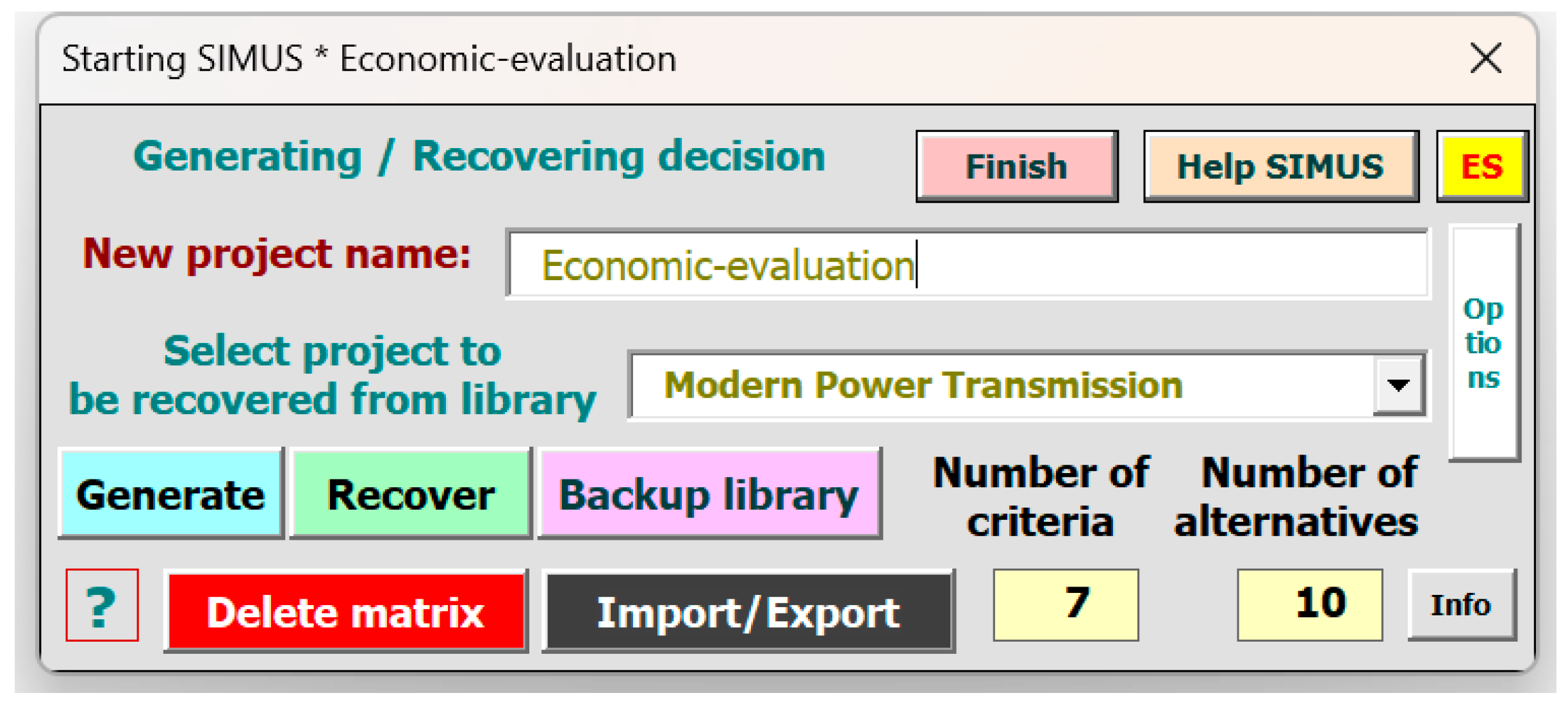
STEP 1: Create a project and enter the number of criteria and alternatives as shown in Figure 7.

Figure 7.
Criteria and alternatives in SIMUS.
STEP 2: Create and normalize a decision matrixThe results were the same as in Table 6.
STEP 3: Start analysis, then export the efficient result matrix (ERM) and the project dominance matrix (PDM). The results are detailed in Table 11 and Table 12.
Table 11.
Normalized efficient result matrix.
Table 12.
Project dominance matrix.
Final Result in ERM and NET in PDM are the scores of 10 projects from two perspectives based on linear programming and mathematical calculations by the SIMUS method. A high score represents a suitable program.
5.3.3. Comparative Analysis of Evaluation Result
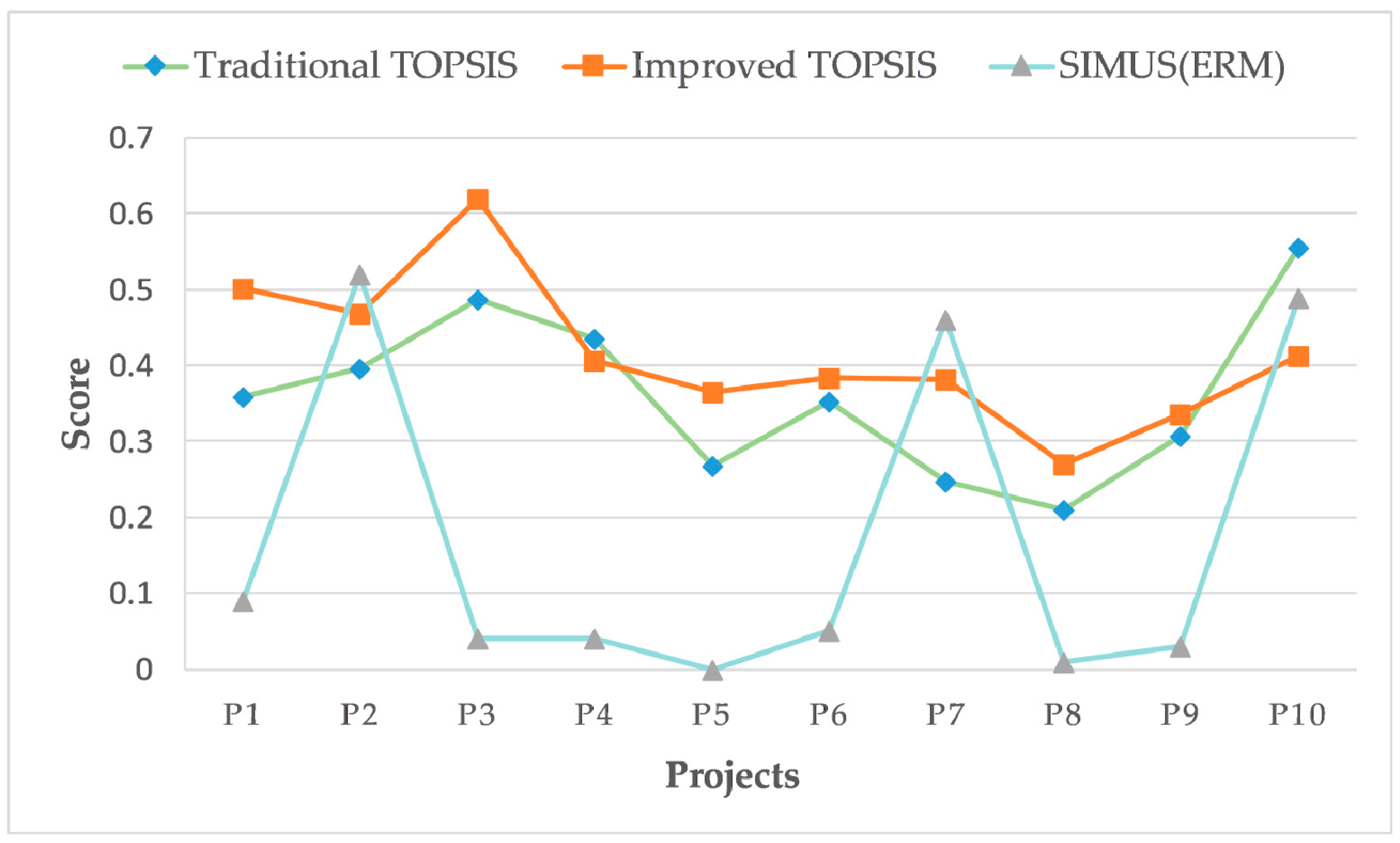
All four sets of scores (traditional and improved relative closeness, NET, and Final Result) were obtained by three different methods or perspectives to rank the example projects, as shown in Table 13. The rankings obtained by the ERM and the DPM are identical. A comparison of the results of the three methods is shown in Figure 8.
Table 13.
Comparison of evaluation scores and rankings.
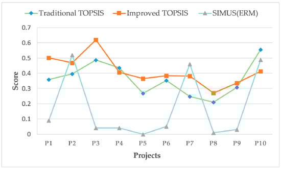
Figure 8.
Comparison of evaluation scores.
Differing methods often lead to varying rankings and preferences in MCDA. Using appropriate coefficients to test the similarity of the rankings would promote a better, more responsible decision [49]. ρ Spearman, τ Kendall, and γ Goodman-Kruskal coefficients are commonly used to check the similarity of rankings [50].
In the comparison analysis using traditional coefficients, the effect of the placement of a pair of adjacent alternatives on similarity is the same for each position in the ranking. In rank correlation analysis using traditional coefficients, interchanging the top two rankings has a commensurate effect to swapping the bottom two on the outcome [51]. This is not rational in MCDA. Hence, a new coefficient WS is proposed to compare the similarity between the rankings, making the differences within the top-ranked intervals more significant [52]:
where is a value of the similarity coefficient, is a length of ranking, and and mean the place in the ranking for - element in respectively ranking and ranking . The result of the WS coefficient is detailed in Table 14.
Table 14.
WS coefficient between the three rankings.
The comparison results are shown in Table 13 and Table 14. The rankings of all three methods have some relatively strong correlation, which follows common sense. The higher correlation between traditional TOPSIS and improved TOPSIS may be because they both use the composite weights derived in the previous section, whereas the SIMUS method focuses on iterating to find the best in the objective data through linear programming. The highest score in the SIMUS method is also because performs well in and . The weights of and in comprehensive weights are very small, so is not ranked as high in the TOPSIS method.
It can be seen in Table 13 that there are some deviations in the ranking results formed by the improved TOPSIS and the traditional TOPSIS. For example, the rankings of and in the two sets of results differ considerably, which is due to the more significant correlation in the indicator system. The improved TOPSIS method is not affected by correlation and magnitude. In contrast, the traditional Euclidean distance is affected by correlation, which leads to the problem of reversed ordering.
In summary, both the individual and comparative analyses have effectively demonstrated the rationality and feasibility of the improved TOPSIS method based on the weighted Mahalanobis distance and the absolute ideal solution proposed in this paper in the economic evaluation of power systems.
6. Conclusions
This paper proposes a comprehensive evaluation method based on improved TOPSIS and BWM-anti-entropy weighting. It applies to the power transmission system, which benefits the investment decision and management. The conclusions are as follows:
- The economic comprehensive evaluation model enhances the tedious process of the traditional AHP method of two-by-two comparison of criteria, and the consistency and reliability of the results are higher. While adding objective weights, the optimal coordination of weights is solved by the Nash equilibrium and Lagrange multiplier methods, respectively. Weights become more accurate and reasonable.
- Improving the TOPSIS method using the Mahalanobis distance and comprehensive weights solves the problem of Euclidean distance failure and inverse order when the linear correlation between criteria is high. Applying the Pearson correlation coefficient rather than covariance circumvents the problems caused by covariance’s inconsistency in magnitude between criteria.
- A comprehensive evaluation of the power transmission system economy was achieved by ranking the relative closeness of ten 500 kV transmission projects to the positive and negative ideal projects. The economic evaluation was performed using the traditional TOPSIS, improved TOPSIS, and SIMUS methods for economic integration, respectively. A comparative analysis was implemented to analyze the differences between the three rankings and their causes. The results indicate that this method provides both an economic evaluation of the power transmission systems and a reflection of the closeness of each criterion to the ideal situation. The evaluation criteria system is characterized by its comprehensiveness and objectivity, while the evaluation process is conducted scientifically and reasonably. As a result, the final evaluation conclusion possesses a high degree of credibility.
Based on comprehensive weights, the method improves the TOPSIS by introducing the Mahalanobis distance and Pearson correlation coefficients, which can eliminate the influence of linear correlation. This method is essentially a multi-attribute decision-making (MADM) method that breaks through the limitations of single-dimension weights. The evaluation can also be expanded to include safety factors and sensitivity, etc. The research object can also be expanded to an entire power grid in a region. Hence, this method is widely applied and can be implemented in the economic analysis of additional diverse subjects. The TOPSIS method will be extended to multi-attribute group decision-making issues.
Author Contributions
Methodology, W.Z., J.F., Z.R., X.L., Y.C. and X.X.; Writing—original draft, Y.C.; Writing—review & editing, X.X.; Visualization, S.L.; Supervision, J.L. All authors have read and agreed to the published version of the manuscript.
Funding
This work was supported by the Science and Technology Project of State Grid Sichuan Electric Power Company (521996220002).
Data Availability Statement
No new data were created or analyzed in this study. Data sharing is not applicable to this article.
Conflicts of Interest
The authors declare no conflict of interest.
Appendix A
As shown in Figure A1, using two dimensions as an example, point B is apparently more of an outlier than point A from a statistical point of view. Nevertheless, if we calculate the Euclidean distance of these two points to the center of the point group, point A is more out of the group. This unreasonable conclusion occurs because there is a linear correlation between and . To avoid the negative influence of this correlation, the coordinate system can be rotated counterclockwise by a certain angle into a new coordinate system .
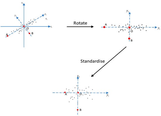
Figure A1.
Mahalanobis distance.
Figure A1.
Mahalanobis distance.
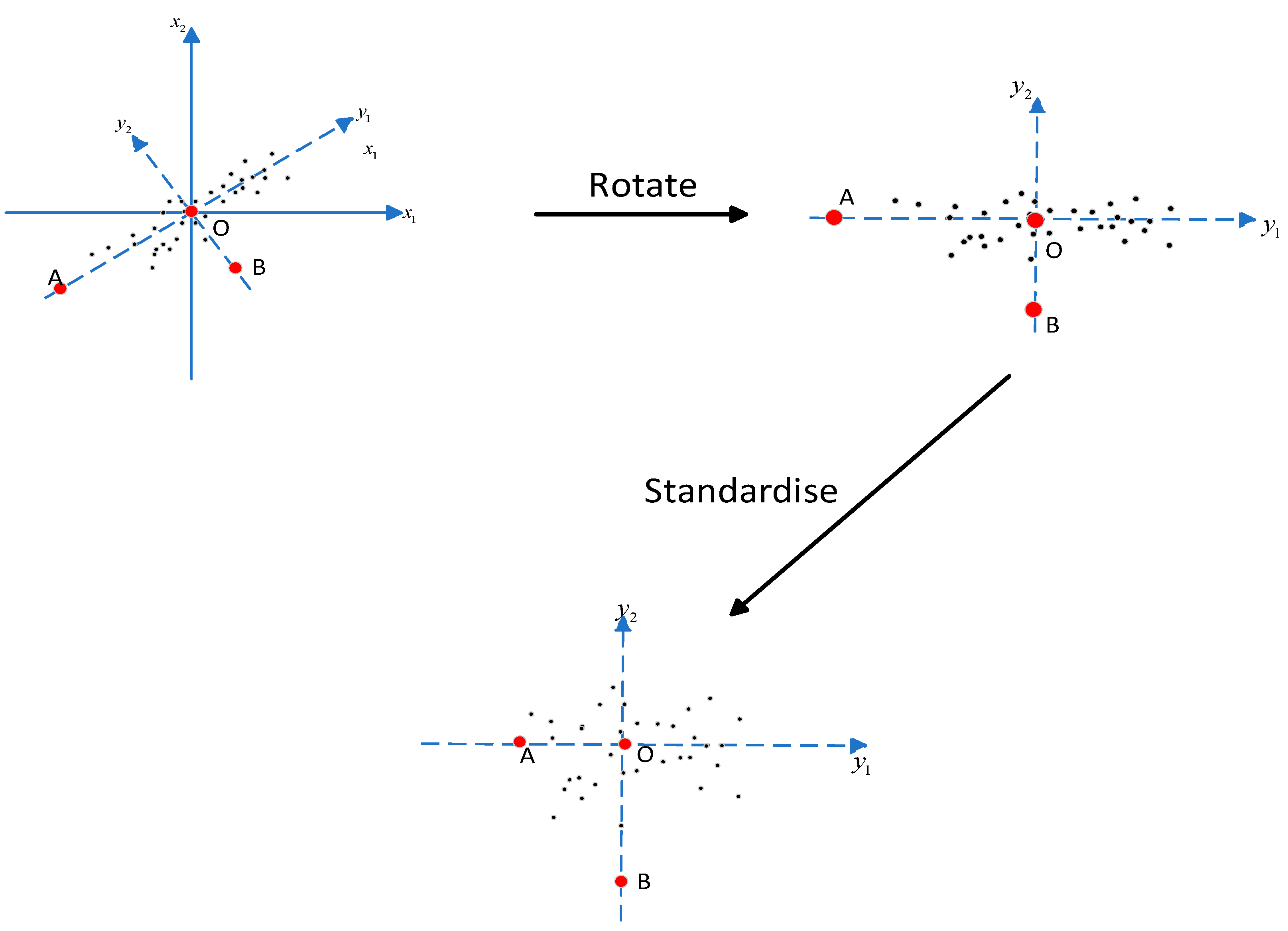
Under the new coordinate system and are uncorrelated, and, after the normalization transformation, the elliptical point group becomes a circular point group. Currently, the Euclidean distance calculated according to the formula is the Mahalanobis distance. It is not difficult to see that the Mahalanobis distance from point to point is shorter than the Mahalanobis distance from point to point .
References
- Fadaeenejad, M.; Saberian, A.M.; Fadaee, M.; Radzi, M.A.M.; Hizam, H.; AbKadir, M.Z.A. The present and future of smart power grid in developing countries. Renew. Sustain. Energy Rev. 2014, 29, 828–834. [Google Scholar] [CrossRef]
- Tinnium, K.; Rastgoufard, P.; Duvoisin, P.F. Probabilistic ranking of large scale transmission projects. Electr. Power Syst. Res. 1997, 42, 21–25. [Google Scholar] [CrossRef]
- Kishore, T.S.; Singal, S.K. Optimal economic planning of power transmission lines: A review. Renew. Sustain. Energy Rev. 2014, 39, 949–974. [Google Scholar] [CrossRef]
- Yang, J.; Xiang, Y.; Wang, Z.; Dai, J.; Wang, Y. Optimal investment decision of distribution network with investment ability and project correlation constraints. Front. Energy Res. 2021, 9, 728834. [Google Scholar] [CrossRef]
- He, Y.; Liu, Y.; Li, M.; Zhang, Y. Benefit evaluation and mechanism design of pumped storage plants under the background of power market reform—A case study of China. Renew. Energy 2022, 191, 796–806. [Google Scholar] [CrossRef]
- Kut, P.; Pietrucha-Urbanik, K. Most Searched Topics in the Scientific Literature on Failures in Photovoltaic Installations. Energies 2022, 15, 8108. [Google Scholar] [CrossRef]
- Pohekar, S.D.; Ramachandran, M. Application of multi-criteria decision making to sustainable energy planning—A review. Renew. Sustain. Energy Rev. 2004, 8, 365–381. [Google Scholar] [CrossRef]
- Samanta, S.; Chakraborty, J.; Dutta, S.B. Village Level Landslide Probability Analysis Based on Weighted Sum Method of Multi-Criteria Decision-Making Process of Darjeeling Himalaya, West Bengal, India. In Geospatial Technology for Environmental Hazards; Shit, P.K., Pourghasemi, H.R., Bhunia, G.S., Das, P., Narsimha, A., Eds.; Springer International Publishing: Cham, Switzerland, 2022; pp. 391–414. [Google Scholar] [CrossRef]
- Tavana, M.; Soltanifar, M.; Santos-Arteaga, F.J. Analytical hierarchy process: Revolution and evolution. Ann. Oper. Res. 2023, 326, 879–907. [Google Scholar] [CrossRef]
- Zahid, K.; Akram, M.; Kahraman, C. A new ELECTRE-based method for group decision-making with complex spherical fuzzy information. Knowl.-Based Syst. 2022, 243, 108525. [Google Scholar] [CrossRef]
- Naseem, A.; Ullah, K.; Akram, M.; Božanić, D.; Ćirović, G. Assessment of Smart Grid Systems for Electricity Using Power Maclaurin Symmetric Mean Operators Based on T-Spherical Fuzzy Information. Energies 2022, 15, 7826. [Google Scholar] [CrossRef]
- Barros, J.R.P.; Melo, A.C.G.; da Silva, A.M.L. An approach to the explicit consideration of unreliability costs in transmission expansion planning. In Proceedings of the 2004 International Conference on Probabilistic Methods Applied to Power Systems, Ames, IA, USA, 12–16 September 2004; pp. 927–932. [Google Scholar]
- Minoia, A.; Ernst, D.; Dicorato, M.; Trovato, M.; Ilic, M. Reference transmission network: A game theory approach. IEEE Trans. Power Syst. 2006, 21, 249–259. [Google Scholar] [CrossRef]
- Chen, P.; Wu, F.; Huang, Z.; Chen, Y. Fuzzy Comprehensive Evaluation of Power Suppliers Based on Combination Weighting. In Proceedings of the 2nd International Conference on Engineering Management and Information Science, EMIS 2023, Chengdu, China, 24–26 February 2023. [Google Scholar] [CrossRef]
- Zhong, Y.; Wang, H.; Lv, H.; Guo, F. A vertical handoff decision scheme using subjective-objective weighting and grey relational analysis in cognitive heterogeneous networks. Ad Hoc Netw. 2022, 134, 102924. [Google Scholar] [CrossRef]
- Behzadian, M.; Khanmohammadi Otaghsara, S.; Yazdani, M.; Ignatius, J. A state-of the-art survey of TOPSIS applications. Expert Syst. Appl. 2012, 39, 13051–13069. [Google Scholar] [CrossRef]
- Ren, L.; Zhang, Y.; Wang, Y.; Sun, Z. Comparative Analysis of a Novel M-TOPSIS Method and TOPSIS. Appl. Math. Res. EXpress 2007, 2007, abm005. [Google Scholar] [CrossRef]
- Aires, R.F.D.F.; Ferreira, L. A new approach to avoid rank reversal cases in the TOPSIS method. Comput. Ind. Eng. 2019, 132, 84–97. [Google Scholar] [CrossRef]
- Yang, B.; Zhao, J.; Zhao, H. A robust method for avoiding rank reversal in the TOPSIS. Comput. Ind. Eng. 2022, 174, 108776. [Google Scholar] [CrossRef]
- Chakraborty, S. TOPSIS and Modified TOPSIS: A comparative analysis. Decis. Anal. J. 2022, 2, 100021. [Google Scholar] [CrossRef]
- Huang, R.; Cui, C.; Sun, W.; Towey, D. Poster: Is Euclidean Distance the best Distance Measurement for Adaptive Random Testing? In Proceedings of the 2020 IEEE 13th International Conference on Software Testing, Validation and Verification (ICST), Porto, Portugal, 24–28 October 2020; pp. 406–409. [Google Scholar]
- Sadeghi, M.; Ameli, A. An AHP decision making model for optimal allocation of energy subsidy among socio-economic subsectors in Iran. Energy Policy 2012, 45, 24–32. [Google Scholar] [CrossRef]
- Kamgar, R.; Hatefi, S.M.; Majidi, N. A Fuzzy Inference System in Constructional Engineering Projects to Evaluate the Design Codes for RC Buildings. Civ. Eng. J. 2018, 4, 2155. [Google Scholar] [CrossRef]
- Sun, L.; Miao, C.; Yang, L. Ecological-economic efficiency evaluation of green technology innovation in strategic emerging industries based on entropy weighted TOPSIS method. Ecol. Indic. 2017, 73, 554–558. [Google Scholar] [CrossRef]
- Bayram, B.Ç. Evaluation of forest products trade economic contribution by entropy-TOPSIS: Case study of Turkey. BioResources 2020, 15, 1419–1429. [Google Scholar] [CrossRef]
- Yang, J.; Dong, X.; Liu, S. Safety Risks of Primary and Secondary Schools in China: A Systematic Analysis Using AHP–EWM Method. Sustainability 2022, 14, 8214. [Google Scholar] [CrossRef]
- He, Z.; Cao, H.; Hu, Q.; Zhang, Y.; Nan, X.; Li, Z. Optimization of apple irrigation and N fertilizer in Loess Plateau of China based on ANP-EWM-TOPSIS comprehensive evaluation. Sci. Hortic. 2023, 311, 111794. [Google Scholar] [CrossRef]
- Zhang, Y.; Khan, S.U.; Swallow, B.; Liu, W.; Zhao, M. Coupling coordination analysis of China’s water resources utilization efficiency and economic development level. J. Clean. Prod. 2022, 373, 133874. [Google Scholar] [CrossRef]
- Ma, Y.; Xu, L.; Cai, J.; Cao, J.; Zhao, F.; Zhang, J. A novel hybrid multi-criteria decision-making approach for offshore wind turbine selection. Wind Eng. 2021, 45, 1273–1295. [Google Scholar] [CrossRef]
- Peng, J.; Zhang, J. Urban flooding risk assessment based on GIS- game theory combination weight: A case study of Zhengzhou City. Int. J. Disaster Risk Reduct. 2022, 77, 103080. [Google Scholar] [CrossRef]
- Basilio, M.P.; De Freitas, J.G.; Kämpffe, M.G.F.; Bordeaux Rego, R. Investment portfolio formation via multicriteria decision aid: A Brazilian stock market study. J. Model. Manag. 2018, 13, 394–417. [Google Scholar] [CrossRef]
- Evers, S.; Goossens, M.; De Vet, H.; Van Tulder, M.; Ament, A. Criteria list for assessment of methodological quality of economic evaluations: Consensus on Health Economic Criteria. Int. J. Technol. Assess. Health Care 2005, 21, 240–245. [Google Scholar] [CrossRef]
- He, Y.; Liu, W.; Jiao, J.; Guan, J. Evaluation method of benefits and efficiency of grid investment in China: A case study. Eng. Econ. 2018, 63, 66–86. [Google Scholar] [CrossRef]
- Chang, K.-P. Corporate Finance: A Systematic Approach; Springer Nature: Singapore, 2023. [Google Scholar] [CrossRef]
- Rezaei, J. Best-worst multi-criteria decision-making method. Omega 2015, 53, 49–57. [Google Scholar] [CrossRef]
- Al-Harbi, K.M.A.-S. Application of the AHP in project management. Int. J. Proj. Manag. 2001, 19, 19–27. [Google Scholar] [CrossRef]
- Basílio, M.P.; Pereira, V.; Costa, H.G.; Santos, M.; Ghosh, A. A Systematic Review of the Applications of Multi-Criteria Decision Aid Methods (1977–2022). Electronics 2022, 11, 1720. [Google Scholar] [CrossRef]
- Ayan, B.; Abacıoğlu, S.; Basilio, M.P. A Comprehensive Review of the Novel Weighting Methods for Multi-Criteria Decision-Making. Information 2023, 14, 285. [Google Scholar] [CrossRef]
- Zhang, W.; Lu, J.; Zhang, Y. Comprehensive Evaluation Index System of Low Carbon Road Transport Based on Fuzzy Evaluation Method. Procedia Eng. 2016, 137, 659–668. [Google Scholar] [CrossRef]
- Wang, W.; Li, H.; Hou, X.; Zhang, Q.; Tian, S. Multi-Criteria Evaluation of Distributed Energy System Based on Order Relation-Anti-Entropy Weight Method. Energies 2021, 14, 246. [Google Scholar] [CrossRef]
- Lai, C.; Chen, X.; Chen, X.; Wang, Z.; Wu, X.; Zhao, S. A fuzzy comprehensive evaluation model for flood risk based on the combination weight of game theory. Nat. Hazards 2015, 77, 1243–1259. [Google Scholar] [CrossRef]
- Rockafellar, R.T. Lagrange Multipliers and Optimality. Siam Rev. 1993, 35, 183–238. [Google Scholar] [CrossRef]
- Dezert, J.; Tchamova, A.; Han, D.; Tacnet, J.-M. The SPOTIS Rank Reversal Free Method for Multi-Criteria Decision-Making Support. In Proceedings of the 2020 IEEE 23rd International Conference on Information Fusion (FUSION), Rustenburg, South Africa, 6–9 July 2020; pp. 1–8. [Google Scholar] [CrossRef]
- Papathanasiou, J.; Ploskas, N. Multiple Criteria Decision Aid: Methods, Examples and Python Implementations; Springer International Publishing: Cham, Switzerland, 2018; Volume 136. [Google Scholar] [CrossRef]
- Asuero, A.G.; Sayago, A.; González, A.G. The Correlation Coefficient: An Overview. Crit. Rev. Anal. Chem. 2006, 36, 41–59. [Google Scholar] [CrossRef]
- Sałabun, W. The Characteristic Objects Method: A New Distance-based Approach to Multicriteria Decision-making Problems. J. Multi-Criteria Decis. Anal. 2015, 22, 37–50. [Google Scholar] [CrossRef]
- Valencia Polytechnic University, INGENIO, Valencia, Spain; Munier, N. A New Approach to the Rank Reversal Phenomenon in MCDM with the SIMUS Method. Mult. Criteria Decis. Mak. 2016, 11, 137–152. [Google Scholar] [CrossRef]
- Munier, N.; Hontoria, E.; Jiménez-Sáez, F. Strategic Approach in Multi-Criteria Decision Making: A Practical Guide for Complex Scenarios; Springer International Publishing: Cham, Switzerland, 2019; Volume 275. [Google Scholar] [CrossRef]
- Ishizaka, A.; Siraj, S. Are multi-criteria decision-making tools useful? An experimental comparative study of three methods. Eur. J. Oper. Res. 2018, 264, 462–471. [Google Scholar] [CrossRef]
- Mulliner, E.; Malys, N.; Maliene, V. Comparative analysis of MCDM methods for the assessment of sustainable housing affordability. Omega 2016, 59, 146–156. [Google Scholar] [CrossRef]
- Blest, D.C. Rank Correlation—An Alternative Measure. Aust. Htmlent Glyphamp Asciiamp N. Z. J. Stat. 2000, 42, 101–111. [Google Scholar] [CrossRef]
- Krzhizhanovskaya, V.V.; Závodszky, G.; Lees, M.H.; Dongarra, J.J.; Sloot, P.M.A.; Brissos, S.; Teixeira, J. (Eds.) Computational Science—ICCS 2020. In Proceedings of the 20th International Conference, Amsterdam, The Netherlands, 3–5 June 2020; Proceedings, Part II. Springer International Publishing: Cham, Switzerland, 2020; Volume 12138. [Google Scholar] [CrossRef]


Disclaimer/Publisher’s Note: The statements, opinions and data contained in all publications are solely those of the individual author(s) and contributor(s) and not of MDPI and/or the editor(s). MDPI and/or the editor(s) disclaim responsibility for any injury to people or property resulting from any ideas, methods, instructions or products referred to in the content. |
© 2023 by the authors. Licensee MDPI, Basel, Switzerland. This article is an open access article distributed under the terms and conditions of the Creative Commons Attribution (CC BY) license (https://creativecommons.org/licenses/by/4.0/).