
Conventional Dissolved Gases Analysis in Power Transformers: Review

 ,
, 
Abstract
:1. Introduction
2. International Standard Developed Techniques
- Incipient Fault Types, Frank M. Clark, 1933–1962;
- Dörnenburg Ratios, E. Dörnenburg, 1967, 1970;
- Potthoff’s Scheme, K. Potthoff, 1969;
- Absolute limits, various sources, early 1970;
- Shank’s Visual Curve method, 1970s;
- Trilinear Plot Method, 1970;
- Key Gas Method, David Pugh, 1974;
- Duval’s Triangle, Michel Duval, 1974;
- Rogers Ratios, R.R. Rogers, 1975;
- Method MSS, 1975;
- Glass Criterion, R.M Glass, 1977;
- Trend Analysis, various sources, early 1980s;
- Church Logarithmic Nomograph, J.O. Church, 1980;
- IEEE C57.104, Limits, rates and total dissolved combustible gas (TDCG), 1978–1991;
- IEC 60599 Ratios, Limits and gassing rates, 1999;
- CIGRE TF 15.01.01, 1999;
- Duval’s Pentagon, Michel Duval, 2014;
- CIGRE TB 771-Advances in DGA interpretation, 2019;
- IEEE EI Mag-New sub-zones for arcing in paper and in oil in Pentagons and Triangle 1, 2022;
- IEEE EI Mag-New sub-zones for carbonization of paper C in Pentagon 2 and Triangle 5, 2023.
- Amount of Key Gases, California State University (CSUS);
- RD 153-34.0-46.302-00 procedural guidelines Russian;
- GATRON method Germany;
- ETRA square Japan;
- Total Combustible Gases, Doble Engineering.
2.1. Key Gas
2.2. Dornenburg
2.3. Rogers
2.4. IEC
2.5. Duval Triangle
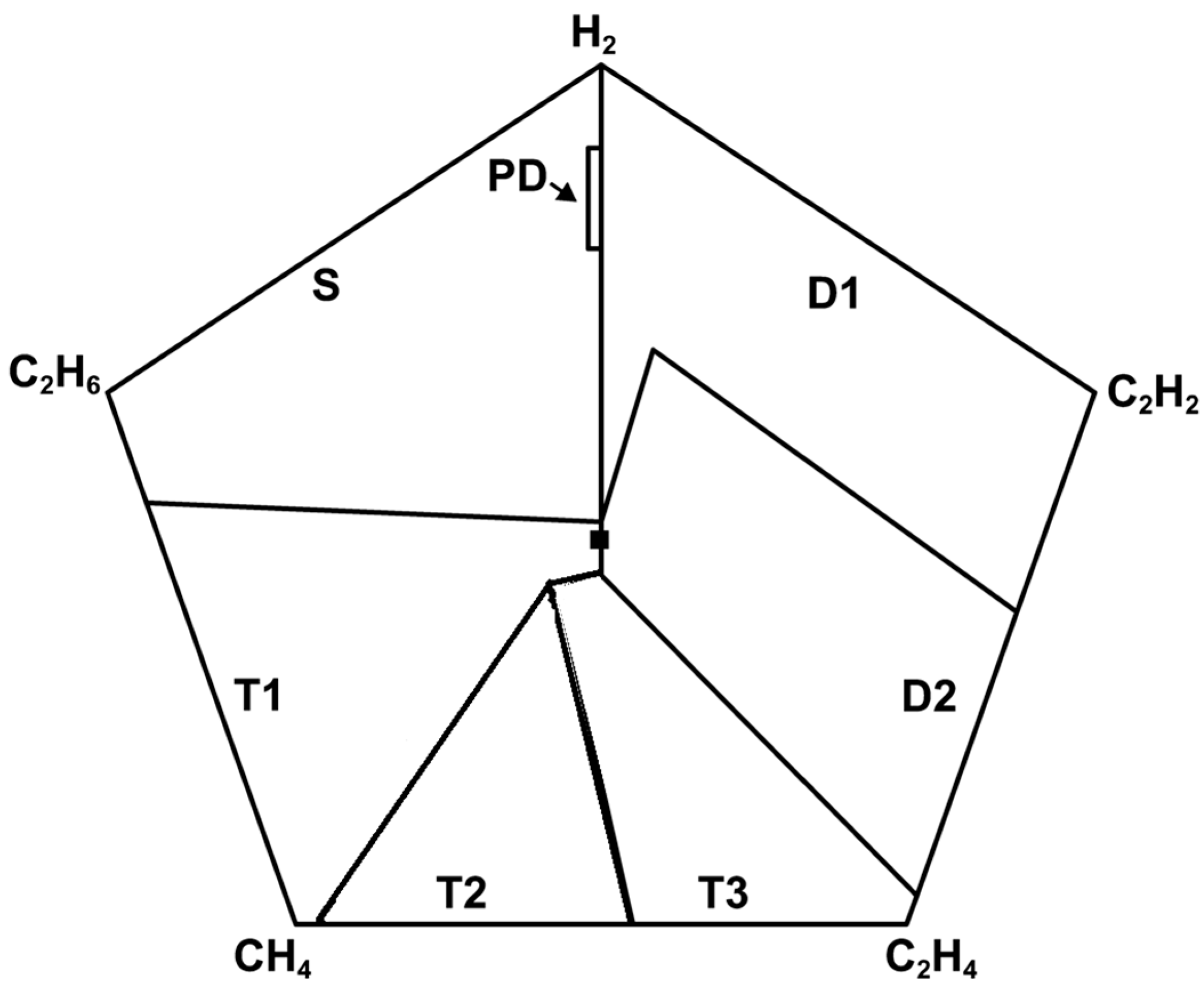
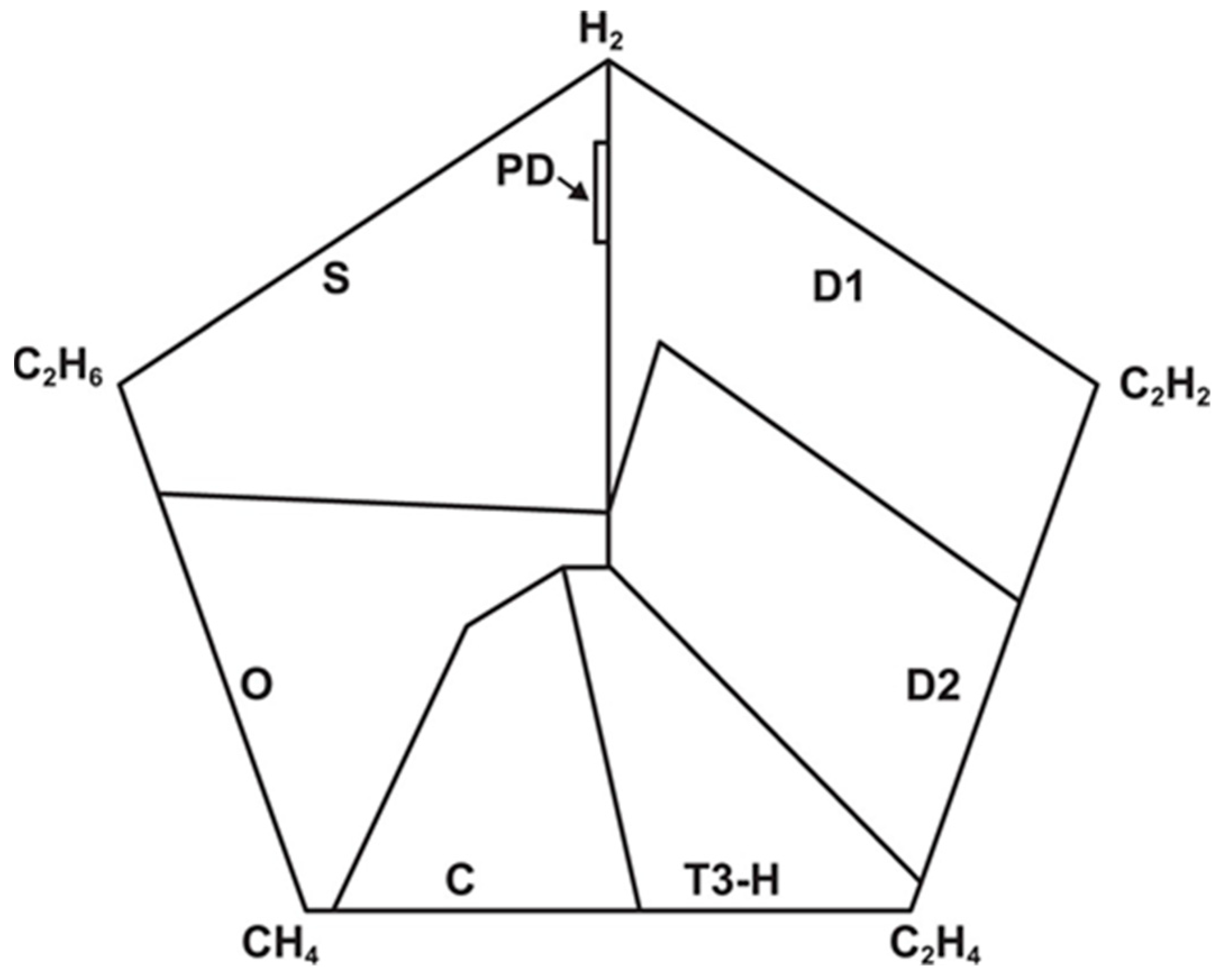
2.6. Duval Pentagon
2.7. Others Methods
2.7.1. Three Rates Technique TRT
2.7.2. Heptagon Graph
3. Results
- Precision: This metric measures how much we can trust a model when it predicts that an example belongs to a certain class:
- Recall: This metric measures the ratio of failures that were correctly identified for a specific class:
- F1-Score: This metric is the harmonic mean between accuracy and recall:
- Accuracy: This metric is the fraction of predictions that the model got right:
- Support: This will give the information of the number of cases in analysis.
- True Positive (TP): model correctly predicts the positive class (prediction and actual, both are positive);
- True Negative (TN): model correctly predicts the negative class (prediction and actual, both are negative);
- False Positive (FP): model gives the wrong prediction of the negative class (predicted-positive, actual-negative);
- False Negative (FN): model wrongly predicts the positive class (predicted-negative, actual-positive).
3.1. Key Gas
3.2. Dornenburg
3.3. Rogers
3.4. IEC
3.5. Duval Triangle
3.6. Duval Pentagon
4. Discussion
5. Conclusions
Author Contributions
Funding
Data Availability Statement
Conflicts of Interest
Appendix A

| Nº | Dissolved Gas Concentration (ppm) | ||||||||
|---|---|---|---|---|---|---|---|---|---|
| H2 | CH4 | C2H6 | C2H4 | C2H2 | CO | CO2 | Equip. | Ref. | |
| 1 | 292.58 | 38.39 | 3.87 | 0.84 | 0 | 161.54 | 523.68 | P | [16] |
| 2 | 522.2 | 43.21 | 16.73 | 1.02 | 1.01 | 158.6 | 2251.3 | P | [16] |
| 3 | 529.75 | 58.96 | 18.12 | 5.06 | 1.27 | 160.5 | 2263.98 | P | [16] |
| 4 | 2525.3 | 130.55 | 14.25 | 1.53 | 0 | 612.17 | 2687.13 | P | [16] |
| 5 | 3417.62 | 131.42 | 14.36 | 1.22 | 0 | 428.03 | 2770.29 | P | [16] |
| 6 | 5869.58 | 175.21 | 16.45 | 1.45 | 0 | 624.47 | 3684.56 | P | [16] |
| 7 | 4966.14 | 145.66 | 15.33 | 1.28 | 0 | 503.42 | 3397.51 | P | [16] |
| Nº | Dissolved Gas Concentration (ppm) | ||||||||
|---|---|---|---|---|---|---|---|---|---|
| H2 | CH4 | C2H6 | C2H4 | C2H2 | CO | CO2 | Equip. | Ref. | |
| 1 | 96 | 20.61 | 5.4 | 15.82 | 38.57 | 367 | 854 | P | [16] |
| 2 | 89 | 20.01 | 6.16 | 16.36 | 39.4 | 354 | 874 | p | [16] |
| 3 | 78 | 20 | 11 | 13 | 28 | 0 | 784 | P | [15] |
| 4 | 305 | 100 | 33 | 161 | 541 | 440 | 3700 | P | [15] |
| 5 | 1230 | 163 | 27 | 233 | 692 | 130 | 115 | P | [15] |
| 6 | 645 | 86 | 13 | 110 | 317 | 74 | 114 | P | [15] |
| 7 | 60 | 10 | 4 | 4 | 4 | 780 | 7600 | R | [15] |
| 8 | 95 | 10 | 0 | 11 | 39 | 122 | 467 | P | [15] |
| 9 | 385 | 60 | 8 | 53 | 159 | 465 | 1250 | R | [15] |
| 10 | 4230 | 690 | 5 | 196 | 1180 | 438 | 791 | R | [15] |
| 11 | 7600 | 1230 | 318 | 836 | 1560 | 4970 | 4080 | R | [15] |
| 12 | 595 | 80 | 9 | 89 | 244 | 524 | 2100 | P | [15] |
| 13 | 120 | 25 | 1 | 8 | 40 | 500 | 1600 | R | [15] |
| 14 | 6454 | 2313 | 121 | 2159 | 6432 | 3628 | 225 | R | [15] |
| 15 | 2177 | 1049 | 207 | 440 | 705 | 4571 | 3923 | R | [15] |
| 16 | 1790 | 580 | 321 | 336 | 619 | 956 | 4250 | R | [15] |
| 17 | 1330 | 10 | 20 | 66 | 182 | 231 | 1820 | P | [15] |
| Nº | Dissolved Gas Concentration (ppm) | ||||||||
|---|---|---|---|---|---|---|---|---|---|
| H2 | CH4 | C2H6 | C2H4 | C2H2 | CO | CO2 | Equip. | Ref. | |
| 1 | 134.78 | 34.7 | 4.5 | 40.54 | 94.1 | 53.1 | 89.76 | P | [16] |
| 2 | 207.6 | 44.14 | 3.8 | 80.9 | 139 | 29.62 | 331.7 | P | [16] |
| 3 | 440 | 89 | 19 | 304 | 757 | 299 | 1190 | P | [15] |
| 4 | 545 | 130 | 16 | 153 | 239 | 660 | 2850 | P | [15] |
| 5 | 7150 | 1440 | 97 | 1210 | 1760 | 608 | 2260 | P | [15] |
| 6 | 120 | 31 | 0 | 66 | 94 | 48 | 271 | R | [15] |
| 7 | 755 | 229 | 32 | 404 | 460 | 845 | 5580 | P | [15] |
| 8 | 5100 | 1430 | 0 | 1140 | 1010 | 117 | 197 | R | [15] |
| 9 | 1570 | 1110 | 175 | 1780 | 1830 | 135 | 602 | P | [15] |
| 10 | 3090 | 5020 | 323 | 3800 | 2540 | 270 | 400 | P | [15] |
| 11 | 1820 | 405 | 35 | 365 | 634 | 1010 | 8610 | P | [15] |
| 12 | 535 | 160 | 16 | 305 | 680 | 172 | 338 | R | [15] |
| 13 | 8200 | 3790 | 250 | 4620 | 5830 | 31 | 85 | R | [15] |
| 14 | 260 | 215 | 35 | 334 | 277 | 130 | 416 | P | [15] |
| 15 | 75 | 15 | 7 | 14 | 26 | 105 | 322 | P | [15] |
| 16 | 530 | 345 | 85 | 266 | 250 | 3900 | 20,000 | R | [15] |
| 17 | 60 | 5 | 2 | 21 | 21 | 188 | 2510 | P | [15] |
| 18 | 90 | 28 | 8 | 31 | 32 | 1380 | 11,700 | R | [15] |
| 19 | 220 | 77 | 22 | 170 | 240 | 1800 | 13,800 | R | [15] |
| 20 | 5900 | 1500 | 68 | 1200 | 2300 | 750 | 335 | R | [15] |
| 21 | 2800 | 2800 | 234 | 3500 | 3600 | 92 | 718 | R | [15] |
| 22 | 99 | 170 | 20 | 200 | 190 | 140 | 1160 | R | [15] |
| 23 | 1500 | 395 | 28 | 395 | 323 | 365 | 576 | P | [15] |
| 24 | 20,000 | 13,000 | 1850 | 29,000 | 57,000 | 2600 | 2430 | P | [15] |
| 25 | 305 | 85 | 25 | 197 | 130 | 813 | 8380 | R | [15] |
| 26 | 1900 | 530 | 35 | 383 | 434 | 1890 | 7570 | R | [15] |
| 27 | 110 | 62 | 90 | 140 | 250 | 680 | 6470 | R | [15] |
| 28 | 3700 | 1690 | 128 | 2810 | 3270 | 22 | 86 | P | [15] |
| 29 | 2770 | 660 | 54 | 712 | 763 | 522 | 1490 | P | [15] |
| 30 | 245 | 120 | 18 | 131 | 167 | 829 | 4250 | R | [15] |
| 31 | 1170 | 255 | 18 | 312 | 325 | 5 | 1800 | P | [15] |
| 32 | 4419 | 3564 | 668 | 2861 | 2025 | 909 | 9082 | R | [15] |
| 33 | 810 | 580 | 111 | 570 | 490 | 1100 | 6800 | R | [15] |
| 34 | 5000 | 1200 | 83 | 1000 | 1100 | 140 | 265 | R | [15] |
| Nº | Dissolved Gas Concentration (ppm) | ||||||||
| H2 | CH4 | C2H6 | C2H4 | C2H2 | CO | CO2 | Equip. | Ref. | |
| 1 | 6.82 | 10.13 | 3.81 | 74.85 | 0 | 662.43 | 5871.86 | P | [16] |
| 2 | 14 | 33.3 | 8 | 20.1 | 0 | 101 | 654 | P | [16] |
| 3 | 87 | 223.6 | 49.6 | 121.1 | 0 | 62 | 498 | P | [16] |
| 4 | 78 | 196.3 | 46.1 | 109.3 | 0 | 51 | 384 | P | [16] |
| 5 | 22.04 | 171.05 | 91.29 | 182.04 | 0 | 1651.57 | 16390.39 | P | [16] |
| 6 | 1270 | 3450 | 520 | 1390 | 8 | 483 | 44500 | P | [15] |
| 7 | 3420 | 7870 | 1500 | 6990 | 33 | 573 | 4640 | P | [15] |
| 8 | 48 | 610 | 29 | 10 | 0 | 1900 | 970 | P | [15] |
| 9 | 12 | 18 | 4 | 4 | 0 | 559 | 1710 | P | [15] |
| 10 | 66 | 60 | 2 | 7 | 0 | 76 | 90 | P | [15] |
| 11 | 14 | 44 | 124 | 7 | 1 | 128 | 2746 | P | [15] |
| 12 | 2031 | 149 | 20 | 3 | 0 | 556 | 3008 | R | [15] |
| 13 | 480 | 1075 | 298 | 1132 | 0 | 464 | 1000 | R | [15] |
| Nº | Dissolved Gas Concentration (ppm) | ||||||||
|---|---|---|---|---|---|---|---|---|---|
| H2 | CH4 | C2H6 | C2H4 | C2H2 | CO | CO2 | Equip. | Ref. | |
| 1 | 82.74 | 108.92 | 28.06 | 249.8 | 3.91 | 809.04 | 2053.72 | P | [16] |
| 2 | 3.11 | 6.61 | 3.23 | 36.43 | 0.26 | 296.54 | 2367.99 | P | [16] |
| 3 | 3.05 | 5.84 | 3.38 | 37.28 | 0.27 | 256.61 | 2970.88 | P | [16] |
| 4 | 3.82 | 7.93 | 3.37 | 52.68 | 0.13 | 406.24 | 2770.54 | P | [16] |
| 5 | 8800 | 64,064 | 72,128 | 95,650 | 0 | 290 | 90,300 | P | [15] |
| 6 | 6709 | 10,500 | 1400 | 17,700 | 750 | 290 | 1500 | P | [15] |
| 7 | 290 | 966 | 299 | 1810 | 57 | 72 | 756 | P | [15] |
| 8 | 2500 | 10,500 | 4790 | 13,500 | 6 | 530 | 2310 | P | [15] |
| 9 | 400 | 940 | 210 | 820 | 24 | 390 | 1700 | P | [15] |
| 10 | 6 | 2990 | 29,990 | 26,076 | 67 | 6 | 26 | P | [15] |
| 11 | 290 | 1260 | 231 | 820 | 8 | 228 | 826 | P | [15] |
| 12 | 1550 | 2740 | 816 | 5450 | 184 | 1140 | 9360 | R | [15] |
| 13 | 3910 | 4290 | 626 | 6040 | 1230 | 1800 | 11,500 | R | [15] |
| 14 | 12,705 | 23,498 | 6047 | 34,257 | 5188 | 4004 | 8539 | R | [15] |
| 15 | 1 | 8 | 8 | 100 | 6 | 300 | 5130 | R | [15] |
| 16 | 300 | 700 | 280 | 1700 | 36 | 760 | 9250 | R | [15] |
| 17 | 107 | 143 | 34 | 222 | 2 | 193 | 1330 | P | [15] |
References
- ASTM D1305-99; Specification for Electrical Insulating Paper and Paperboard. The American Society for Testing and Materials (ASTM): Conshohocken, PA, USA, 2004.
- IEC 60554-3-3; Specification for Cellulosic Papers for Electrical Purposes. International Electrotechnical Commission (IEC): Geneva, Switzerland, 1984.
- ASTM D3487-16E1; Standard Specification for Mineral Insulating Oil Used in Electrical Apparatus. The American Society for Testing and Materials (ASTM): Conshohocken, PA, USA, 2016.
- Meyers, S.D.; Kelly, J.J.; Parrish, E.R.H. A Guide to Transformer Maintenance; VDOC.PUB: Akron, Ohio, 1981; pp. 323–388. ISBN 0-939320-00-2. [Google Scholar]
- Colton, R. Combustible Gas Testing on Large Oil Filled Transformers. In Proceedings of the 9th Electrical Insulation Conference, Boston, MA, USA, 8–11 September 1969; pp. 115–118. [Google Scholar] [CrossRef]
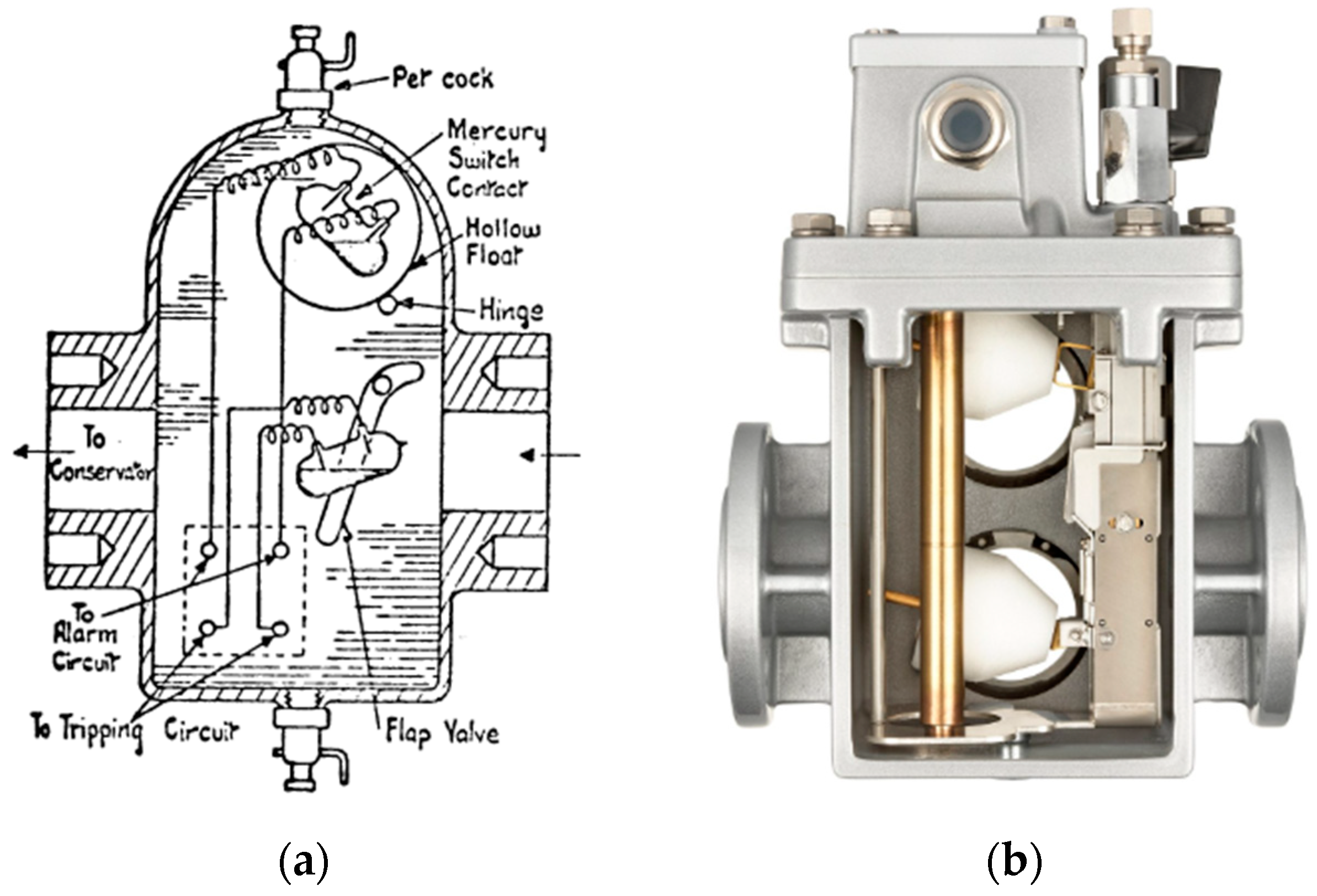
- Messko Msafe Relay Buchholz, Mr Industry. Available online: https://www.reinhausen.com/productdetail/buchholz-relays/messko-msafe (accessed on 4 July 2023).
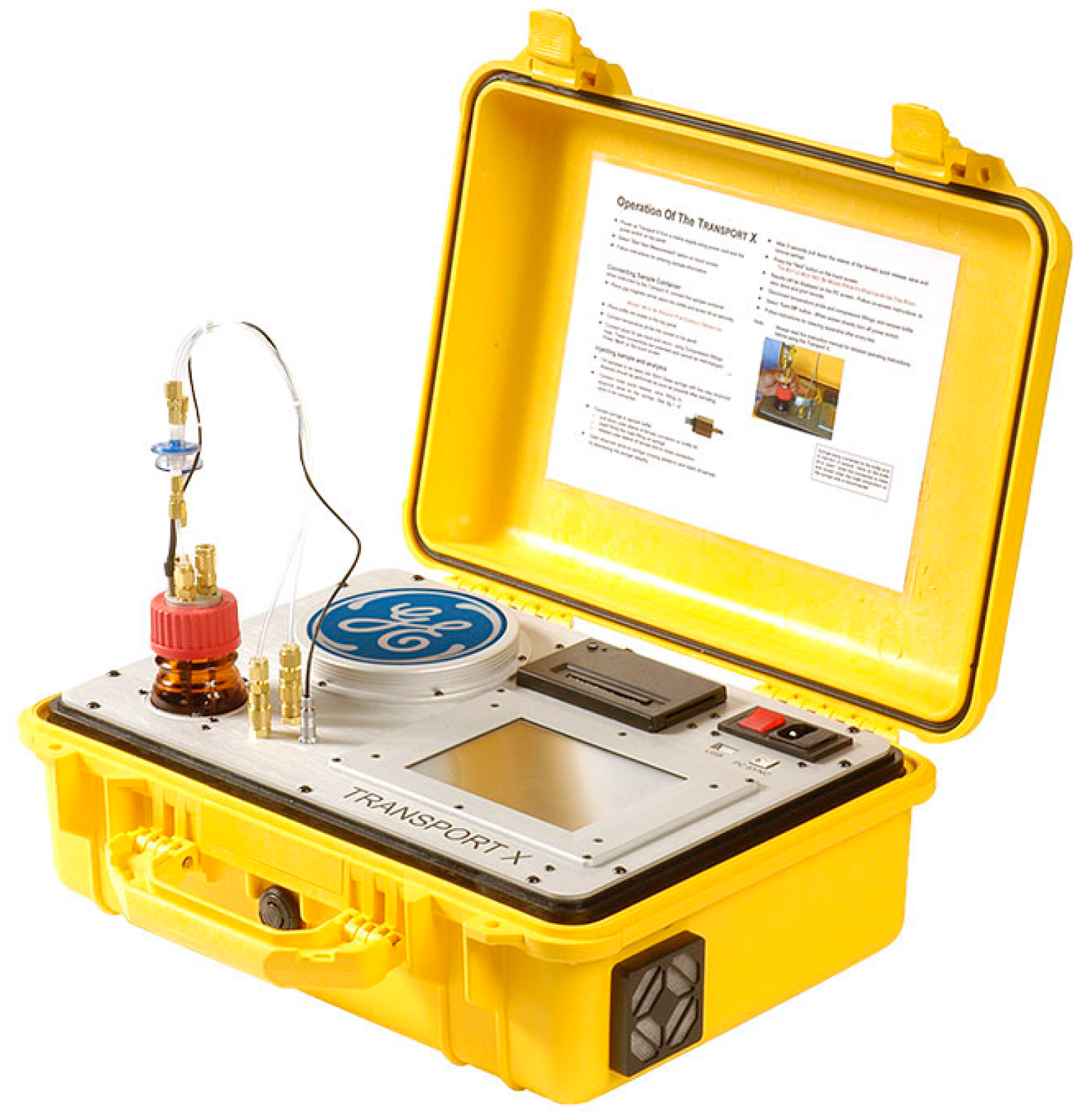
- Kelman TRANSPORT X. Available online: https://www.gegridsolutions.com/MD/CATALOG/TRANSPORTX.HTM (accessed on 4 July 2023).
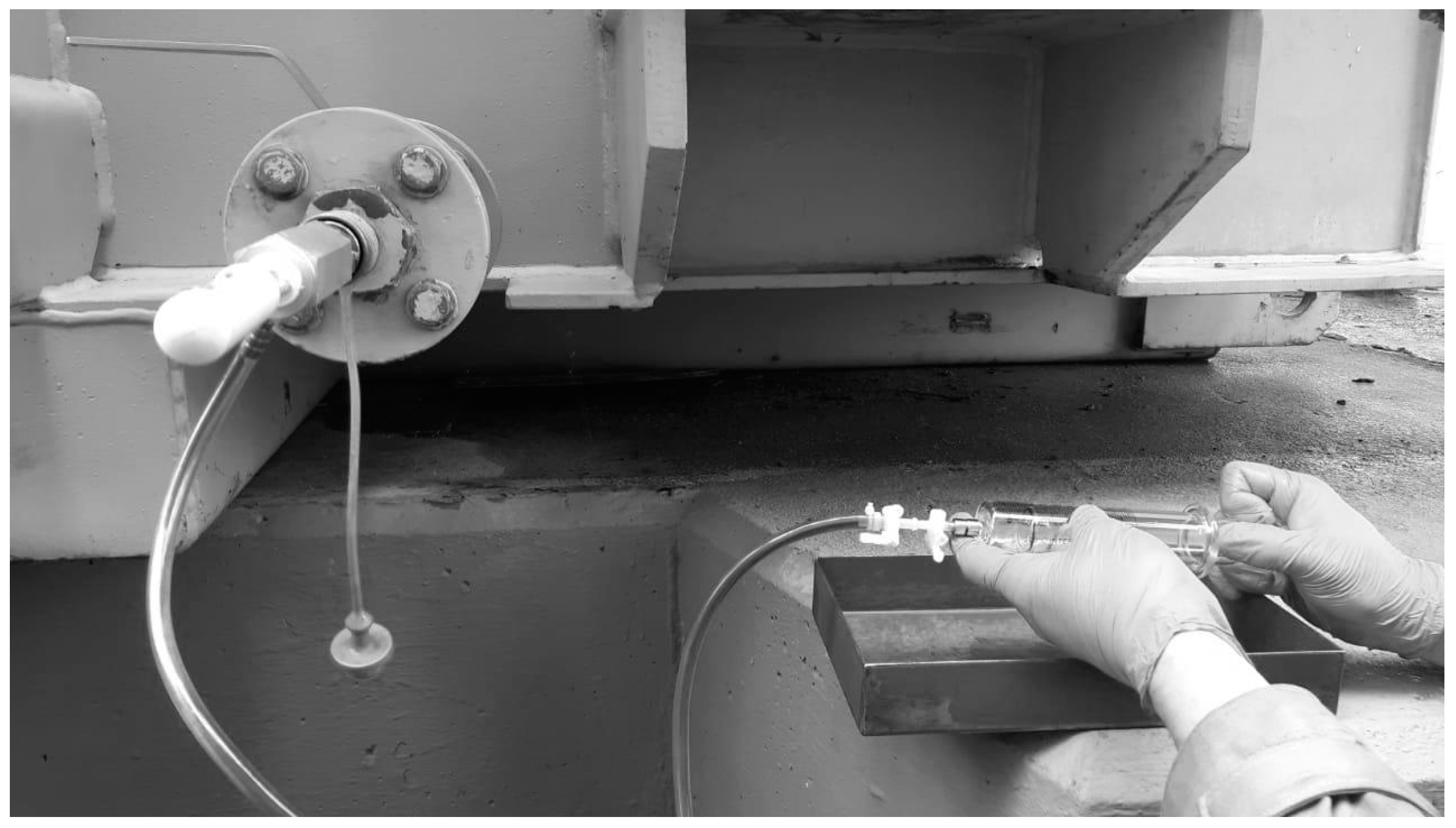
- CEI EN 60475; Method of Sampling Insulating Liquids. International Electrotechnical Commission (IEC): Geneva, Switzerland, 2011.
- VDE 0370-9; Oil-Filled Electrical Equipment—Sampling of Gases and Analysis of Free and Dissolved Gases—Guidance. International Electrotechnical Commission (IEC): Geneva, Switzerland, 2011.
- Vahidi, B.; Teymouri, A. Quality Confirmation Tests for Power Transformer Insulation Systems; Springer: Berlin/Heidelberg, Germany, 2019; pp. 1–12. [Google Scholar]
- Rogers, R.R. IEEE and IEC Codes to Interpret Faults in Transformers Using Gas in Oil Analysis. IEEE Trans. Electr. Insul. 1978, 75, 349–354. [Google Scholar] [CrossRef]
- C57.104-1991; IEEE Guide for the Interpretation of Gases Generated in Oil-Immersed Transformers. The Institute of Electrical and Electronics Engineers (IEEE) Standard: Piscataway, NJ, USA, 1991.
- ASTM D3612-02; Standard Test Method for Analysis of Gases Dissolved in Eletric Insulation Oil by Gas Chromatography. The American Society for Testing and Materials (ASTM): Conshohocken, PA, USA, 2009.
- Keshavamurthy, H.C.; Ravindra, D. An attempt to investigate transformer failure by Dissolved Gas Analysis. J. CPRI 2017, 13, 607–614. [Google Scholar]
- Duval, M.; Depablo, A. Interpretation of Gas-In-Oil Analysis Using New IEC Publication 60599 And IEC TC 10 Databases. IEEE Electr. Insul. Mag. 2001, 17, 31–41. [Google Scholar] [CrossRef]
- Zeng, B.; Guo, J.; Zhu, W.; Xiao, Z.; Yuan, F.; Huang, S. A transformer Fault Diagnosis Model Based on Hybrid Grey Wolf Optmizer and LS-SVM. Energies 2019, 12, 4170. [Google Scholar] [CrossRef]
- N’Cho, J.S.; Fofana, I.; Hadjadj, Y.; Beroual, A. Review of Physicochemical-Based Diagnostic Techniques for Assessing Insulation Condition in Aged Transformers. Energies 2016, 9, 367. [Google Scholar] [CrossRef]
- Syafruddin, H.; Nugroho, H.P. Dissolved Gas Analysis (DGA) for Diagnosis of Fault in Oil-Immersed Power Transformers A Case Study. In Proceedings of the IEEE 4th International Conference on Electrical, Telecommunication and Computer Engineering (ELTICOM), Medan, Indonesia, 3–4 September 2020. [Google Scholar] [CrossRef]
- Ali, M.S.; Bakar, A.H.A.; Omar, A.; Jaafar, A.S.A.; Mohamed, S.H. Conventional Methods of Dissolved Gas Analysis Using Oil-Immersed Power Transformer for Fault Diagnosis: A Review. Eletr. Power Syst. Res. 2023, 216, 109064. [Google Scholar] [CrossRef]
- Faiz, J.; Soleimani, M. Dissolved Gas Analysis Evaluation in Eletric Power Transformers Using Conventional Methods a Review. IEEE Trans. Dielectr. Electr. Insul. 2017, 24, 1239–1248. [Google Scholar] [CrossRef]
- Swanasri, C.; Wannapring, E.; Swanasri, T. Dissolved Gas Analysis Methods for Distribution Transformers. In Proceedings of the 13th International Conference on Electrical Engineering/Electronics, Computer, Telecommunications and Information Technology (ECTI-CON), Chiang Mai, Thailand, 28 June–1 July 2016. [Google Scholar] [CrossRef]
- Wattakapaiboon, W.; Pattanadech, N. The State of the Art for Dissolved Gas Analysis Based on Interpretation Techniques. In Proceedings of the International Conference on Condition Monitoring and Diagnosis (CMD), Xi’an, China, 25–28 September 2016. [Google Scholar] [CrossRef]
- Junior, H.F.; Costa, J.G.S.; Olivas, J.L. A Review of Monitoring Methods for Predictive Maintenance of Electric Power Transformers Based on Dissolved Gas Analysis. Renew. Sustain. Energy Rev. 2015, 46, 201–209. [Google Scholar] [CrossRef]
- Sun, H.C.; Huang, Y.C.; Huang, C.M. A Review of Dissolved Gas Analysis in Power Transformers. Energy Procedia 2012, 14, 1220–1225. [Google Scholar] [CrossRef]
- IEC 60599 Ed. 3.0 b:2015; Mineral Oil-Impregnated Electrical Equipment in Service—Guide to the Interpretation of Dissolved and Free Gases Analysis. International Electrotechnical Commission (IEC): Geneva, Switzerland, 2015.
- Duval, M. Fault Gases Formed in Oil-Filled Breathing EHV Power Transformers—the Interpretation of Gas Analysis Data. IEEE PAS 1974, 1974, 1–4. [Google Scholar]
- C57.139-2015; IEEE Guide for Dissolved Gas Analysis in Transformer Load Tap Changers. The Institute of Electrical and Electronics Engineers (IEEE) Standard: New York, NY, USA, 2015.
- Duval, M. The Duval Triangle for Load Tap Changers, Non-Mineral Oils and Low Temperature Faults in Transformers. IEEE Electr. Insul. Mag. 2008, 24, 22–29. [Google Scholar] [CrossRef]
- Akbari, A.; Setayeshmehr, A.; Borsi, H.; Gockenbach, E. A Software Implementation of the Duval Triangle Method. In Proceedings of the Conference Record of the 2008 IEEE International Symposium on Electrical Insulation, Vancouver, BC, Canada, 9–12 June 2008. [Google Scholar] [CrossRef]
- Mansour, D.A. A New Graphical Technique for the Interpretation of Dissolved Gas Analysis in Power Transformers. In Proceedings of the 2012 Annual Report Conference on Electrical Insulation and Dielectric Phenomena, Montreal, QC, Canada, 14–17 October 2012; pp. 195–198. [Google Scholar] [CrossRef]
- Gamez, C. Dissolved Gas Analysis, Measurements and Interpretations Power Transformer Condition Monitoring and Diagnosis. In Power Transformer Condition Monitoring and Diagnosis; The Institute of Engineering and Tecnology (IET): London, UK, 2018; pp. 1–38. [Google Scholar] [CrossRef]
- Mansour, D.A. Development of A New Graphical Technique for Dissolved Gas Analysis in Power Transformers Based on The Five Combustible Gases. IEEE Trans. Dielectr. Electr. Insul. 2015, 22, 2507–2512. [Google Scholar] [CrossRef]
- Duval, M.; Lamarre, L. The Duval Pentagon—A New Complementary Tool for the Interpretation of Dissolved Gas Analysis in Transformers. IEEE Electr. Insul. Mag. 2014, 30, 9–12. [Google Scholar] [CrossRef]
- Cheim, L.; Duval, M.; Haider, S. Combined Duval Pentagons: A Simplified Approach. Energies 2020, 13, 2859. [Google Scholar] [CrossRef]
- Duval, M.; Alzieu, E.; Banovic, M.; Bhumiwat, S.; Boman, P.; Buchacz, T.; Dale, A.M.; Djurik, B.; Grisaru, M.; Heizmann, T.; et al. Advances in DGA Interpretation; CIGRE: Paris, France, 2019; ISBN 978-2-85873-473-3. [Google Scholar]
- Saha, T.K.; Purkait, P. Transformer Ageing—Monitoring and Estimation Techniques; Wiley-IEEE Press: Pondicherry, India, 2017; pp. 211–243. [Google Scholar] [CrossRef]
- Zhang, Y.; Tang, Y.; Liu, Y.; Liang, Z. Fault Diagnosis of Transformer Using Artificial Intelligence: A Review; School of Information Science, Guangdong University of Finance and Economics: Guangzhou, China; School of Electric Power, South China University of Technology: Guangzhou, China, 2022. [Google Scholar] [CrossRef]
- Li, Y. The State of the Art in Transformer Fault Diagnosis with Artificial Intelligence and Dissolved Gas Analysis: A Review of the Literature; School of Electrical and Electronics Engineering, North China Electric Power University: Beijing, China, 2023. [Google Scholar] [CrossRef]
- Gouda, O.E.; El-Hoshy, S.H.; El-Tamaly, H.E. Proposed Three Ratios Technique for the Interpretation of Mineral Oil Transformers Based Dissolved Gas Analysis. IET Gener. Transm. Distrib. 2018, 12, 2650–2661. [Google Scholar] [CrossRef]
- Gouda, O.E.; El-Hoshy, S.H.; El-Tamaly, H.H. Proposed Heptagon Graph for DGA Interpretation of Oil Transformers. IET Gener. Transm. Distrib. 2018, 12, 490–498. [Google Scholar] [CrossRef]
- Gouda, O.E.; El-Hoshy, S.H.; Ghoneim, S.S.M. Enhancing, the Diagnostic Accuracy of DGA Techniques Based on IEC-TC10 and Related Databases. IEEE Access 2021, 9, 118031–118041. [Google Scholar] [CrossRef]


| Gas Type | Concetration (ppm) |
|---|---|
| Hydrogen (H2) | 100 |
| Methane (CH4) | 120 |
| Carbon Monoxide (CO) | 350 |
| Carbon Dioxide (CO2) | 2500 |
| Acetylene (C2H2) | 1 |
| Ethylene (C2H4) | 50 |
| Ethane (C2H6) | 65 |
| Suggested Fault Diagnosis | CH4 H2 | C2H2 C2H4 | C2H2 CH4 | C2H6 C2H2 |
|---|---|---|---|---|
| Thermal Decomposition | >1 | <0.75 | <0.3 | >0.4 |
| Partial Discharge (Low intensity) | <0.1 | Not significant | <0.3 | >0.4 |
| Arcing (High intensity) | 0.1 to 1 | >0.75 | >0.3 | <0.4 |
| Fault | CH4 H2 | C2H6 CH4 | C2H4 C2H6 | C2H2 C2H4 |
|---|---|---|---|---|
| Normal | ≥0.1 and <1 | <1 | <1 | <0.5 |
| Partial discharge | ≤0.1 | <1 | <1 | <0.5 |
| Overheating < 150 °C | ≥1 and <3 or ≥3 | <1 | <1 | <0.5 |
| Overheating 150 °C to 200 °C | ≥1 and <3 or ≥3 | ≥1 | <1 | <0.5 |
| Overheating 200 °C to 300 °C | >0.1 and <1 | ≥1 | <1 | <0.5 |
| General conductor overheating | >0.1 and <1 | <1 | ≥1 and <3 | <0.5 |
| Winding circulating currents | ≥1 and <3 | <1 | ≥1 and <3 | <0.5 |
| Core and tank circulating currents | ≥1 and <3 | <1 | ≥3 | <0.5 |
| Flashover without power follow through | >0.1 and <1 | <1 | <1 | ≥0.5 and <3 |
| Arc with power follow through | >0.1 and <1 | <1 | ≥1 and <3 or ≥3 | ≥0.5 and <3 or ≥3 |
| Continuous sparking to floating potential | >0.1 and <1 | <1 | ≥3 | ≥3 |
| Partial discharge with tracking | ≤0.1 | <1 | <1 | ≥0.5 and <3 or ≥3 |
| Fault | C2H2 C2H4 | CH4 H2 | C2H4 C2H6 |
|---|---|---|---|
| Normal | <0.1 | ≥0.1 and <1 | <1 |
| Low-energy density arcing-PD | <0.1 | <0.1 | <1 |
| Arcing high-energy discharge | ≥1 and ≤3 | ≥0.1 and ≤1 | >3 |
| Low temperature thermal | <0.1 | ≥0.1 and ≤1 | ≥1 and ≤3 |
| Thermal < 700 °C | <0.1 | >1 | ≥1 and ≤3 |
| Thermal > 700 °C | <0.1 | >1 | >3 |
| Fault | C2H2 C2H4 | CH4 H2 | C2H4 C2H6 |
|---|---|---|---|
| No fault | <0.1 | ≥0.1 and <1 | <1 |
| Partial discharge of low-energy density | <0.1 | <0.1 | ≥1 and <3 |
| Partial discharge of high-energy density | ≥0.1 and <3 | <0.1 | ≥1 and <3 |
| Discharge of low energy | ≥0.1 and <3 or ≥3 | ≥0.1 and <1 | <1 |
| Discharge of high energy | ≥0.1 and <3 | ≥0.1 and <1 | <1 |
| Thermal fault of temperature < 150 °C | <0.1 | ≥0.1 and <1 | <1 |
| Thermal fault of low temperature range 150 °C to 300 °C | <0.1 | ≥1 | >3 |
| Thermal fault of medium temperature range 300 °C to 700 °C | <0.1 | ≥1 | >3 |
| Thermal fault of high temperature range > 700 °C | <0.1 | ≥1 | >3 |
| Fault | C2H2 C2H4 | CH4 H2 | C2H4 C2H6 |
|---|---|---|---|
| Partial discharges (PD) | NS | <0.1 | <0.2 |
| Discharge of low energy (D1) | >1 | ≥0.1 and ≤0.5 | >1 |
| Discharge of high energy (D2) | ≥0.6 and ≤2.5 | ≥0.1 and ≤1 | >2 |
| Thermal fault t < 300 °C (T1) | NS | ≥1 but NS | <1 |
| Thermal fault 300 °C < t < 700 °C (T2) | <0.1 | >1 | ≥1 and ≤4 |
| Thermal fault t > 700 °C (T3) | <0.2 | >1 | >4 |
| Fault | R1 | R2 | R3 |
|---|---|---|---|
| T3 | R1 > 0.05 | R2 ≤ 1 | R3 < 0.5 |
| T2 | R1 > 0.05 | 1 ≤ R2 ≤ 3.5 | R3 < 0.5 |
| T1 | R1 > 0.05 | R2 > 3.5 | R3 < 0.5 |
| T0 | 0.05 ≤ R1 ≤ 0.9 | NS. | R3 < 0.05 |
| PD1 | R1 ≤ 0.05 | R2 > 1 | R3 < 0.5 |
| PD2 | R1 ≤ 0.05 | R2 > 1 | R3 ≥ 0.5 |
| D1 | R1 ≥ 0.05 | R2 > 3.5 | R3 ≥ 0.5 |
| D2 | R1 ≤ 0.9 | R2 ≤ 3.5 | R3 ≥ 0.5 |
| DT | R1 > 0.9 | R2 ≤ 3.5 | R3 ≥ 0.5 |
| Techinique | Fault Types | |||||
|---|---|---|---|---|---|---|
| T1 | T2 | T3 | PD | D1 | D2 | |
| Duval Triangle T1 | Thermal fault < 300 °C | Thermal fault 300–700 °C | Thermal fault > 700 °C | Partial Discharge | Low-energy discharge | High-energy discharge |
| Dornenburg | Thermal decomposition (T) | Partial Discharge (PD) | Energy Discharge–Arcing (D) | |||
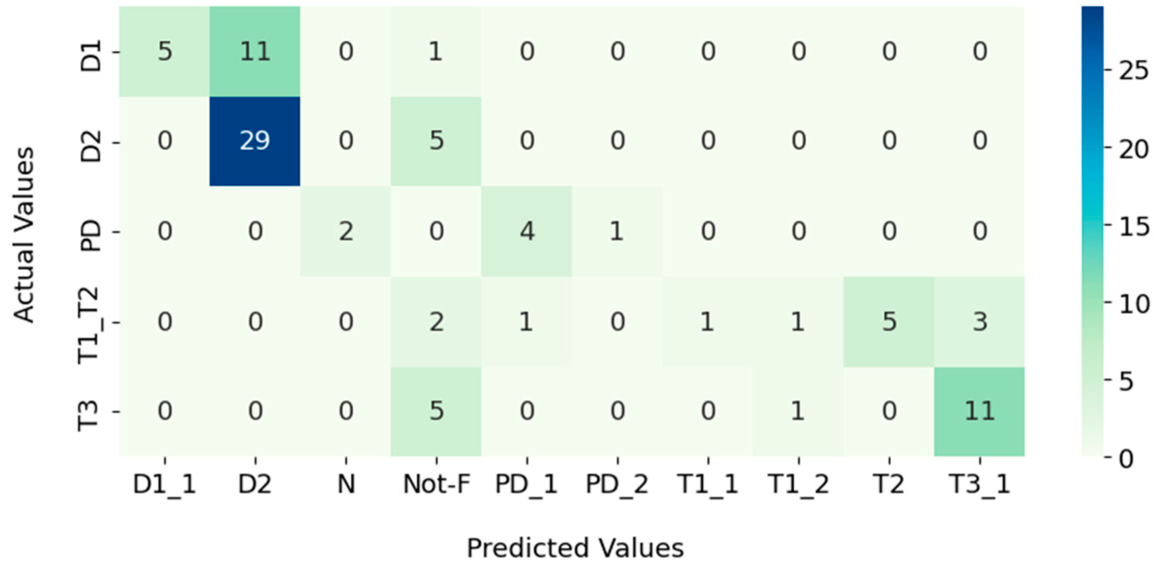
| Rogers | Thermal fault of low temperature < 150 °C (T1_1) | Winding circulation current (T2) | Core and tank circulation current (T3_1) | Partial discharge with low energy (PD_1) | Continuous Sparking (D1_1) | Arc with power follows through (D2) |
| Thermal fault of temperature range 150–200 °C (T1_2) | Insulated conductor overheating (T3_2) | Partial discharge with tracking (PD_2) | Flashover (D1_2) | |||
| Thermal fault of temperature range 200–300 °C (T1_3) | ||||||
| Rogers IEEE | Low temperature thermal (T1) | Thermal < 700 °C (T2) | Thermal > 700 °C (T3) | Low-energy density arcing-(PD) | Arcing-High-energy discharge (D) | |
| IEC ratio method | Thermal fault of temperature < 150 °C (T1_1) | Thermal fault of medium temperature range 300 °C to 700 °C (T2) | Thermal fault of high temperature range > 700 °C (T3) | PD of low-energy density (PD_1) | Discharge with low-energy density (D1) | Discharge with high-energy arcing (D2) |
| Thermal fault of low temperature range 150 °C to 300 °C (T1_2) | PD of high-energy density (PD_2) | |||||
| IEC 60599 ratio method | Thermal fault t < 300 °C (T1) | Thermal fault 300 °C < t < 700 °C (T2) | Thermal fault t > 700 °C (T3) | Partial Discharge (PD) | Discharge of low energy (D1) | Discharge of high energy (D2) |
| Duval Pentagon 1 | Termal fault < 300 °C | Thermal fault 300–700 °C | Thermal fault > 700 °C | Partial Discharge | Low-energy discharge | High-energy discharge |
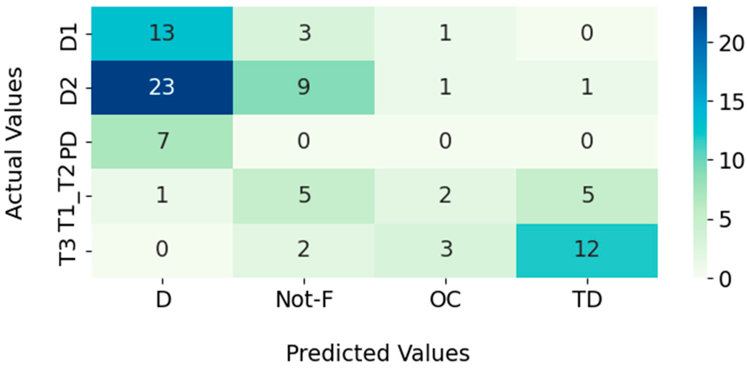
| Key Gas | Thermal degradation (TD) | Partial Discharge (PD) | Arcing (D) | |||
| Overheat cellulose (OC) | ||||||
| Failure | Performance Analysis | |||
|---|---|---|---|---|
| Precision | Recall | F1-Score | Support | |
| D | 0.82 | 0.71 | 0.76 | 51 |
| PD | 0.00 | 0.00 | 0.00 | 8 |
| T | 0.88 | 0.73 | 0.80 | 30 |
| Accuracy | 0.66 | 88 | ||
| Failure | Performance Analysis | |||
|---|---|---|---|---|
| Precision | Recall | F1-Score | Support | |
| D | 1.00 | 0.84 | 0.91 | 51 |
| PD | 0.83 | 0.71 | 0.77 | 7 |
| T | 1.00 | 0.80 | 0.89 | 30 |
| Accuracy | 0.82 | 88 | ||
| Failure | Performance Analysis | |||
|---|---|---|---|---|
| Precision | Recall | F1-Score | Support | |
| D1 | 1.00 | 0.29 | 0.45 | 17 |
| D2 | 0.72 | 0.85 | 0.78 | 34 |
| PD | 0.83 | 0.71 | 0.77 | 7 |
| T1_T2 | 0.88 | 0.54 | 0.67 | 13 |
| T3 | 0.79 | 0.65 | 0.71 | 17 |
| Accuracy | 0.65 | 88 | ||
| Failure | Performance Analysis | |||
|---|---|---|---|---|
| Precision | Recall | F1-Score | Support | |
| D | 1.00 | 0.53 | 0.69 | 51 |
| PD | 0.80 | 0.57 | 0.67 | 7 |
| T1_T2 | 0.75 | 0.46 | 0.57 | 13 |
| T3 | 0.80 | 0.71 | 0.75 | 17 |
| Accuracy | 0.56 | 88 | ||
| Failure | Performance Analysis | |||
|---|---|---|---|---|
| Precision | Recall | F1-Score | Support | |
| D1 | 0.86 | 0.71 | 0.77 | 17 |
| D2 | 0.88 | 0.85 | 0.87 | 34 |
| PD | 0.83 | 0.71 | 0.77 | 7 |
| T1_T2 | 0.70 | 0.54 | 0.61 | 13 |
| T3 | 0.80 | 0.71 | 0.75 | 17 |
| Accuracy | 0.74 | 88 | ||
| Failure | Performance Analysis | |||
|---|---|---|---|---|
| Precision | Recall | F1-Score | Support | |
| D1 | 1.00 | 0.47 | 0.64 | 17 |
| D2 | 0.87 | 0.79 | 0.83 | 34 |
| PD | 0.83 | 0.71 | 0.77 | 7 |
| T1_T2 | 0.47 | 0.62 | 0.53 | 13 |
| T3 | 0.83 | 0.59 | 0.69 | 17 |
| Accuracy | 0.66 | 88 | ||
| Failure | Performance Analysis | |||
|---|---|---|---|---|
| Precision | Recall | F1-Score | Support | |
| D1 | 1.00 | 0.88 | 0.94 | 17 |
| D2 | 0.94 | 1.00 | 0.97 | 34 |
| PD | 0.67 | 0.57 | 0.62 | 7 |
| T1_T2 | 0.60 | 0.46 | 0.52 | 13 |
| T3 | 0.82 | 0.82 | 0.82 | 17 |
| accuracy | 0.83 | 88 | ||
| Failure | Performance analysis | |||
|---|---|---|---|---|
| Precision | Recall | F1-Score | Support | |
| D1 | 0.84 | 0.94 | 0.89 | 17 |
| D2 | 1.00 | 0.88 | 0.94 | 34 |
| PD | 0.83 | 0.71 | 0.77 | 7 |
| T1_T2 | 0.78 | 0.54 | 0.64 | 13 |
| T3 | 0.78 | 0.82 | 0.80 | 17 |
| accuracy | 0.82 | 88 | ||
Disclaimer/Publisher’s Note: The statements, opinions and data contained in all publications are solely those of the individual author(s) and contributor(s) and not of MDPI and/or the editor(s). MDPI and/or the editor(s) disclaim responsibility for any injury to people or property resulting from any ideas, methods, instructions or products referred to in the content. |
© 2023 by the authors. Licensee MDPI, Basel, Switzerland. This article is an open access article distributed under the terms and conditions of the Creative Commons Attribution (CC BY) license (https://creativecommons.org/licenses/by/4.0/).
Share and Cite
Rangel Bessa, A.; Farias Fardin, J.; Marques Ciarelli, P.; Frizera Encarnação, L. Conventional Dissolved Gases Analysis in Power Transformers: Review. Energies 2023, 16, 7219. https://doi.org/10.3390/en16217219
Rangel Bessa A, Farias Fardin J, Marques Ciarelli P, Frizera Encarnação L. Conventional Dissolved Gases Analysis in Power Transformers: Review. Energies. 2023; 16(21):7219. https://doi.org/10.3390/en16217219
Chicago/Turabian StyleRangel Bessa, Alcebíades, Jussara Farias Fardin, Patrick Marques Ciarelli, and Lucas Frizera Encarnação. 2023. "Conventional Dissolved Gases Analysis in Power Transformers: Review" Energies 16, no. 21: 7219. https://doi.org/10.3390/en16217219
APA StyleRangel Bessa, A., Farias Fardin, J., Marques Ciarelli, P., & Frizera Encarnação, L. (2023). Conventional Dissolved Gases Analysis in Power Transformers: Review. Energies, 16(21), 7219. https://doi.org/10.3390/en16217219