Article

Hybrid Framework for Enhanced Dynamic Optimization of Intelligent Completion Design in Multilateral Wells with Multiple Types of Flow Control Devices

Institute of GeoEnergy Engineering, Heriot-Watt University, Edinburgh EH14 4AS, UK
*
Author to whom correspondence should be addressed.
Energies 2023, 16(20), 7189; https://doi.org/10.3390/en16207189
Submission received: 26 September 2023 / Revised: 14 October 2023 / Accepted: 20 October 2023 / Published: 21 October 2023
(This article belongs to the Special Issue Recent Advances in Oil and Gas Recovery and Production Optimisation)

Abstract

:
Multilateral wells (MLWs) equipped with multiple flow control devices (FCDs) are becoming increasingly favored within the oil sector due to their ability to enhance well-to-reservoir exposure and effectively handle unwanted fluid breakthrough. However, combining various types of FCDs in multilateral wells poses a complex optimization problem with a large number of highly correlated control variables and a computationally expensive objective function. Consequently, standard optimization algorithms, including metaheuristic and gradient-based approaches, may struggle to identify an optimal solution within a limited computational resource. This paper introduces a novel hybrid optimization (HO) framework combining particle swarm optimization (PSO) and Simultaneous Perturbation Stochastic Approximation (SPSA). It is developed to efficiently optimize the completion design of MLWs with various FCDs while overcoming the individual limitations of each optimization algorithm. The proposed framework is further enhanced by employing surrogate modelling and global sensitivity analysis to identify critical parameters (i.e., highly sensitive) that greatly affect the objective function. This allows for a focused optimization effort on these key parameters, ultimately enhancing global optimization performance. The performance of the novel optimization framework is evaluated using the Olympus benchmark reservoir model. The model is developed by three intelligent dual-lateral wells, with inflow control devices (ICDs) installed within the laterals and interval control valves (ICVs) positioned at the lateral junctions. The results show that the proposed hybrid optimization framework outperforms all industry-standard optimization techniques, achieving a Net Present Value of approximately USD 1.94 billion within a limited simulation budget of 2500 simulation runs. This represents a substantial 26% NPV improvement compared to the open-hole case (USD 1.54 billion NPV). This improvement is attributed to more efficient water breakthrough management, leading to a notable 24% reduction in cumulative water production and, consequently, a 26% increase in cumulative oil production.

1. Introduction

Over the past few years, there has been a significant trend towards adopting multilateral wells mainly due to their advantages over conventional vertical and horizontal wells. These wells allow for multiple branches to be drilled from a single wellbore, which leads to increased reservoir access, improved production rates, and reduced drilling costs. However, multilateral wells face challenges such as flow imbalances due to reservoir heterogeneity and the “heel-to-toe effect”, which can result in early breakthroughs of unwanted fluids, leading to a decreased overall well performance. To overcome these challenges, flow control devices (FCDs, find the list of abbreviations after Conclusions) are employed to regulate fluid flow rates from well zones, create more uniform pressure profiles along the wellbore branches, and balance inflow, ensuring maximum hydrocarbon recovery from reservoir zones.
Several types of FCDs can be used in smart well completions, including inflow control devices (ICDs), autonomous flow control devices (AFCDs), and interval control valves (ICVs) as shown in Figure 1. ICDs are passive inflow control devices that regulate fluid flow by creating additional pressure drops through specialized flow paths such as labyrinth/helical channels, nozzles/slots, or hybrid [1]. AFCDs operate autonomously and can be classified into (1) autonomous interval control valves (AICVs), which almost completely shut off the flow of unwanted fluid by mechanically self-adjusting their flow area [2]; and (2) autonomous inflow control devices (AICDs), which selectively restrict the flow of unwanted fluid by creating an extra pressure drop after the breakthrough occurs. Two popular types of AICDs commonly used in the industry are the fluidic diode AICD (FD-AICD), which has no moving parts and relies on its special flow channel design to achieve fluid flow control, and the rate-controlled production AICD (RCP-AICD), which consists of a device body, a nozzle, and a free-floating disk that controls production from the nozzle. The movement of the floating disk depends on the fluid viscosity. When a fluid with low viscosity, such as water, flows through the nozzle, the pressure at the nozzle’s entrance drops as per Bernoulli’s principle. As a result, the combined force on the disk causes it to move in the direction of the inlet, partially restricting the flow area [3].
Interval control valves (ICVs) are active surface-controlled devices and can be classified based on their control flexibility to on/off or discrete (i.e., the open area has several positions), and infinitely variable ICVs enable operators to exert zone-by-zone control and implement flexible production strategies to enhance field production. ICVs can also be classified according to their control system, which includes hydraulic, all-electric-, electric–hydraulic, and wireless-controlled ICVs. Control of ICVs can be achieved through reactive or proactive approaches. The reactive strategy adjusts ICVs based on the current parameters of the well and reservoir, reducing the production of undesired fluids in real time [4,5]. While this approach is effective for an immediate response to undesired situations, it generally fails to achieve optimal long-term field management. In contrast, the proactive strategy focuses on anticipating and planning for potential reservoir challenges by optimizing ICV settings in advance to delay unwanted fluids’ breakthrough and maximize recovery. However, this approach relies on accurate reservoir models, which can be challenging due to geological uncertainties that may negatively impact the effectiveness of proactive control strategies [6].
There has been significant research work on dynamic optimization of a single type of FCD (e.g., completions equipped with ICVs or ICDs only). These methods involve coupling a reservoir simulator with an optimization algorithm. Following are some major publications classified based on the employed optimization algorithm: (a) metaheuristic and population-based algorithms [5,7,8,9,10,11,12,13,14,15,16] (b) gradient-based or derivative-based algorithms [17,18,19,20,21], and (c) stochastically estimated gradient-based algorithms [22,23,24,25].
Metaheuristic and population-based algorithms can be effective in achieving global optimization. However, their performance deteriorates rapidly as the number of control variables increases [6]. Gradient-based and stochastic gradient-based algorithms exhibit faster convergence as they use the derivatives of the objective function to guide the search direction; however, they are prone to converging to local optima and are highly affected by the presence of sensitive parameters in the objective function, which results in a poor estimation of the objective function gradients [26]. Furthermore, the efficiency of the gradient-based algorithms is heavily dependent on the initial starting point (guess); with an initial guess far from the optimal solution, the algorithm may fail to converge to the optimal solution within a limited simulation budget [20,27].
The algorithms’ performance can further deteriorate when applied to an optimization problem with control variables of different types as this creates a more complex optimization problem. This complexity arises from the large number of correlated control variables and the computationally demanding objective function [28]. A sequential optimization approach, which involves dividing the problem into subproblems based on the type of control variables and optimizing them sequentially, has been suggested by some researchers to alleviate this issue [29]. However, this approach can lead to a suboptimal solution due to the overlooking of correlation effects between control variables.
Other studies have recommended utilizing a hybrid approach that combines multiple algorithms to achieve better optimization performance. For example, Yang et al. [30] used a differential evolution algorithm (DE) and mesh adaptive direct search (MADS) to simultaneously optimize the well type, number of wells, well locations, and well control strategies. Their hybrid workflow showed superior performance compared to standalone DE and MADS. Fue and Wen [31] successfully combined a genetic algorithm (GA), particle swarm optimization (PSO), and adjoint algorithm in a multiscale optimization framework to solve a reservoir management optimization problem. H. Ma et al. [32] developed a hybrid algorithm that combined steepest ascend (SA) and PSO algorithms to optimize CO2-cyclic solvent injection and waterflooding in post-cold heavy oil production. Tozzo et al. [33] applied variable neighborhood descent (VND), a local search algorithm, to improve solutions obtained from the GA operators to solve the workover rigs scheduling optimization problem. Han et al. [34] applied a combined PSO and MADS algorithms approach in the well placement and control optimization problems of horizontal steam flooding wells. Even though all prior hybrid methods exhibited improved performance in contrast to using standalone algorithms, the search for the optimal solution was still rather random (i.e., no guidance to the optimization algorithms is involved) and relied only on the effectiveness of the individual algorithms employed.
This paper presents a multistage hybrid optimization (HO) framework that employs two distinct algorithms; particle swarm optimization (PSO) and Simultaneous Perturbation Stochastic Approximation (SPSA) to tackle the complex optimization problem that arises when two different types of flow control devices are employed in multilateral wells. The PSO, as a global search algorithm, is utilized in an initial optimization stage to explore the search space to identify promising regions for further investigation. The data generated in this stage are used to build a surrogate model using the radial basis function neural network. Global sensitivity analysis is then performed using the developed surrogate model to divide the parameters into high and low-impact groups, based on their total impacts (effects) on the objective function. A sequential optimization approach is then performed in the second stage by optimizing the high-impact group using PSO, followed by optimization of the remaining control variables using the SPSA algorithm. In the HO, the concentration and direction of optimization endeavors towards enhancing the parameters that hold significant importance in the optimization process. As a result, a guided optimization approach is established, leading to a comprehensive improvement in the performance of global optimization. The proposed optimization framework was tested on a benchmark model “Olympus” and showed superior performance in comparison with the industry-standard optimization techniques.
This paper proceeds as follows. In Section 2, we formulate the optimization problem and provide an overview of the PSO and SPSA algorithms as well as a brief explanation of the radial basis function neural network and global sensitivity analysis tool used. Section 3 presents the proposed hybrid optimization strategy. The results of testing the hybrid optimization framework on the Olympus model and comparison with standard optimization techniques are discussed in Section 4. Finally, Section 5 summarizes the findings.

2. Problem Formulation

The objective of advanced completion design and control in MLWs is to find the optimal settings of multiple types of flow control devices (ICDs and ICVs) to maximize an objective function. The Net Present Value (NPV) is selected as the objective function. It considers oil, water production, and water injection costs as well as the produced water handling costs as outlined in Equation (1):
J x R N x m R N m = f x , m = n = 1 s j = 1 N p r r o q o , j n r p w q w , j n I w = 1 N I c w i q w i , k n   δ t n 1 + b t n
where x is the N x dimensional vector of the decision variables; m is the N m dimensional state vector of the reservoir; n is the n t h time step of the reservoir simulation; s is the total number of simulation steps; and N p r and N I are the number of producers and injectors, respectively. The cost parameters r o , r p w , and c w i represent the oil price and water handling cost both in USD/m3 and the water injection cost, respectively. q o , j n and q w , j n are the oil and water production rates, respectively, of well j at time step n in m3/day. q w i , k n is the water injection rate of well I w at time step n in m3/day. δ t n is the length of the n t h simulation step in days; t n is the simulation time (in years) at the end of the n t h time step; and b is the annual discount rate in decimal (see Nomenclature after Conclusions). The objective function is evaluated using a commercial dynamic reservoir simulator [35] for the specified set of optimization variables and state vectors. The economic values that are used to calculate the NPV are presented in Table 1.

2.1. Particle Swarm Optimization (PSO)

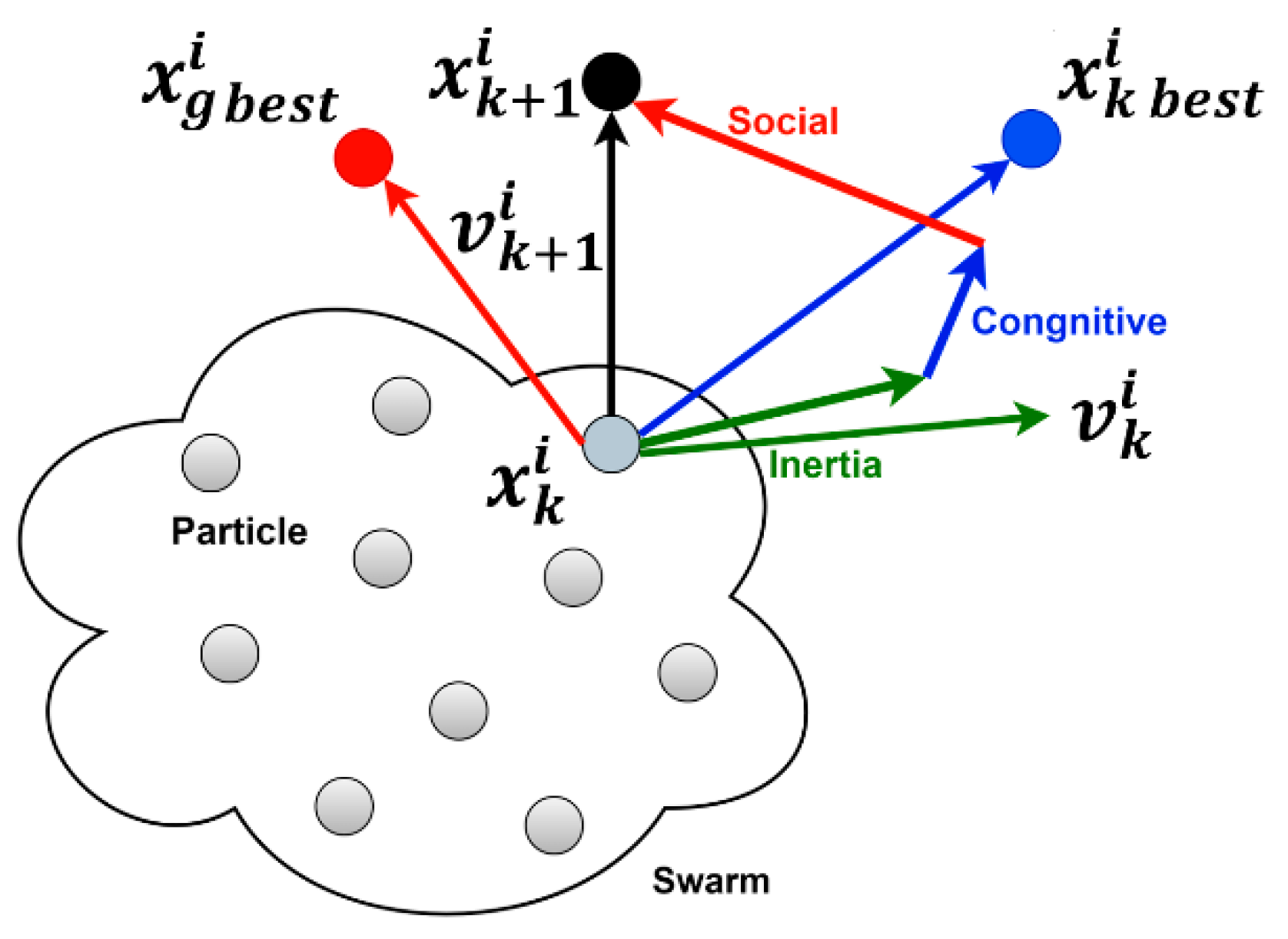
PSO is a metaheuristic, derivative-free, and population-based optimization algorithm inspired by the social behavior of swarms of animals such as birds and fish [36]. In PSO, each possible solution is referred to as a particle ( x k ), while a set of potential solutions (particles) forms a swarm. The particles are randomly scattered at various directions in the search space as shown in Figure 2 and updated iteratively in each iteration ( k ) based on the velocity vector ( v k ) until the maximum number of iterations ( N ) is reached (Equation (2)).
x k + 1 i = x k i + v k + 1 i ,     k = 1 , 2 , 3 , , N   a n d   i = 1 , 2 , 3 , , N p
where N p is the total number of particles or the swarm (population) size. The velocity vector is evaluated every iteration based on three weighting components: the inertia component ( ω I ), cognitive component ( ω c ), and social component ( ω s ) as shown in Equation (3).
v k + 1 i = ω I v k i + ω c R 1 x k   b e s t i x k i + ω s R 2 x g   b e s t i x k i
where R 1   and R 2 are random numbers generated from uniform distribution; x k   b e s t i and x k   g   b e s t i are the best solution for the particle and the global best solution for all particles, respectively. Following Clerc and Kennedy [37], we set the weighting components ω I , ω c , and ω s to 0.729, 1.494, and 1.494, respectively.

2.2. Simultaneous Perturbation Stochastic Approximation (SPSA)

The SPSA algorithm, developed by Spall [39], is a stochastically estimated gradient-based method that operates by simultaneously perturbing all input parameters aiming to reduce the number of objective function evaluations required for calculating gradients. Let J = f x k be the objective function of a dimensional vector of control variables at iteration k where x k = x 1 , x 2 ,   . x p   k T . The SPSA intends to increase the value of the objective function f x k iteratively by adjusting x k as shown by Equation (4):
x k + 1 = x k + α k g ^ k x k
where g ^ k x k is the stochastically approximated gradient of the objective function. To compute the estimate g ^ k x k , the SPSA algorithm generates a random vector k = k 1 ,   k 2   ,   , k p T . Each component in this vector is an independent random variable drawn from a symmetric Bernoulli distribution ±1 with probability ½. g ^ k x k can then be calculated using c k as shown in Equation (5):
g ^ k x k = f x k + c k k f x k c k k 2 c k 1 k 1 , 1 k 2 , . . , 1 k p T
where α k and c k are tuning parameters for the SPSA algorithm and represent the step size and perturbation size, respectively. Spall [39] suggested the following decaying formulas to calculate α k and c k :
α k = a A + k + 1 ϑ
c k = c k + 1 γ
where ϑ , γ , A ,   a , and c are positive real numbers. Spall recommended ϑ and γ to be 0.602 and 0.101, respectively. A is suggested to be 10% of the total number of control variables. a and c are tuning parameters, respectively [40]. Initial analysis, in this work, showed that the SPSA algorithm has a stable performance (less oscillation) with the values of a = 2 and c = 0.5. In this study, we utilize an average stochastic approximated gradient g ^ k ( x k ) ¯ to enhance the accuracy of the search direction estimation [41]. To achieve this, the SPSA algorithm generates n e independent samples of ∆k during each iteration resulting in 2 × n e objective function evaluations. The average stochastic gradient is subsequently calculated by taking the arithmetic mean of an ensemble of n e estimated gradients using the following formula:
g ^ k ( x k ) ¯ = 1 n e j = 1 n e g ^ k x k
The updated parameter x at k + 1 yields:
x k + 1 = x k + α k g ^ k ¯ x k g ^ k ¯ x k
where     is the infinity norm of the vector.

2.3. Surrogate Modelling Using Radial Basis Function (RBF)

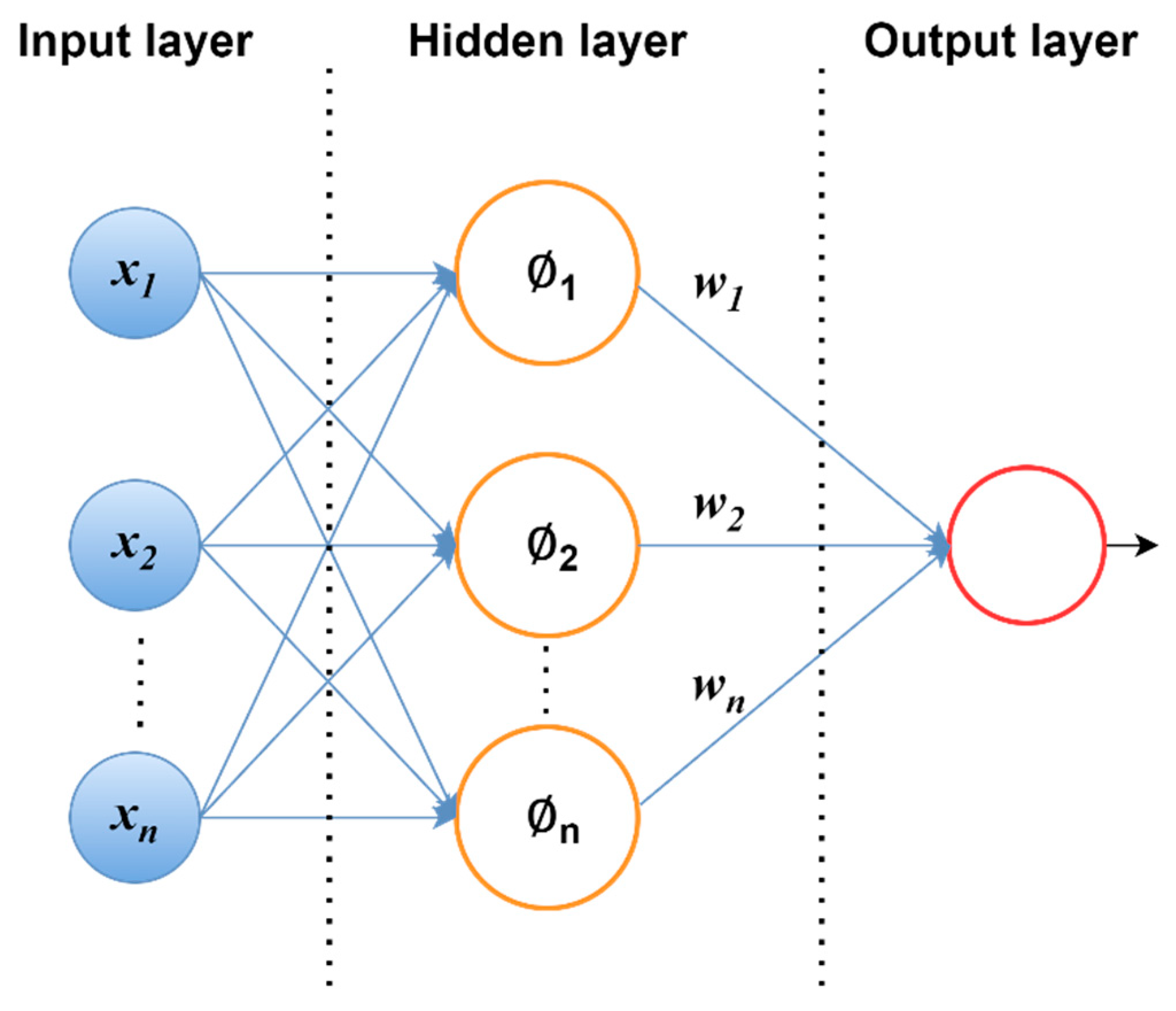
We provide a brief description along with the mathematical configuration of the radial basis function in this section; more detailed information and discussion can be found in [42,43]. The RBF is similar to a multilayer perceptron artificial neural network; however, there are essential differences between the two: (1) The structure of an RBF network is straightforward, encompassing an input layer, a solitary hidden layer comprised of nonlinear processing units, and an output layer featuring linear weights (Figure 3). (2) The number of neurons in the input layer corresponds directly to the number of input variables. (3) The RBF network leverages weightless connections to efficiently propagate inputs from each neuron in the input layer to all neurons in the hidden layer. (4) An inherent strength of the RBF lies in its ability to accurately approximate nonlinear functions, thereby demonstrating robust performance across diverse dimensions. Moreover, the training process for RBF networks exhibits notable simplicity relative to alternative types of artificial neural networks, as it obviates the need for computationally intensive backpropagation for weight optimization. This reduction in the training computational cost significantly enhances the efficiency and practicality of the RBF, rendering it an appealing choice for various applications necessitating function approximation, pattern recognition, and data analysis. In this study, we employ RBF to construct a proxy model that is used only to facilitate the global sensitivity analysis.
The input–output mapping performed by the RBF is described in Equation (10):
J = f x i = i = 1 n w i x i , x p
where: J is the value of the objective function, n is the size of training data, w i   is the weight of each neuron in the hidden layer, x i   is the input parameter vectors, x p is the unit center determined by the clustering algorithm, and   x i , x p is the multivariate Gaussian density function (transfer function), which depends on the distance between   x p and x i , and it is expressed by Equation (11):
x i , x p = e x i x p 2 2 σ j 2
where σ j is a distance scaling parameter, determining the distance in the input space over which the unit has a significant impact. We follow the traditional two-step method of training RBF networks available in the literature. The first step involves applying the nearest-neighbor chain algorithm [44] to determine the centers (centroids) that represent the number of nodes in the hidden layer. In the second step, the bias and connection weights between the hidden layer and the output layer are optimized to minimize the root-mean-square error (RMSE) between the simulator and proxy results as defined in Equation (12). This is accomplished by utilizing the Levenberg–Marquardt algorithm [45] during model training.
RMSE = i = 1 n J i a c t J i p r o x y 2 n
where J i a c t and J i p r o x y are the objective functions (NPV) obtained from the actual reservoir model and the proxy model, respectively; n is the size of the training set.

2.4. Variogram Analysis of Response Surface (VARS)

VARS is a model-based global sensitivity analysis technique developed by Razavi and Gupta [46]. It uses the directional variogram function to quantify the impact of the model parameters (FCD settings) on the objective function (NPV). VARS is selected in this study to perform this task for the following reasons:
(1)
It considers the main, interaction, and total effects of the input variables on the objective function (i.e., higher-order sensitivities), making it a robust tool in complex optimization problems. In contrast, other simplified sensitivity analysis techniques such as one-at-a-time [47], and local sensitivity analysis such as differential sensitivity analysis [48] do not consider these effects together. Applying such simplified techniques in complex optimization problems can result in incorrect and misleading outcomes.
(2)
VARS requires a smaller number of objective function evaluations to estimate the sensitivity indices compared to other global sensitivity analyses such as the Sobol method [49], which makes VARS more computationally efficient [50].
Although VARS demands fewer function evaluations, the procedure of assessing it through a numerical simulator can still be laborious and time-intensive. Consequently, the incorporation of a surrogate model, specifically an RBF-based proxy in this study, becomes essential to facilitate these resource-intensive simulation runs.
Suppose that the objective function of a model is represented by:
J = f x 1 , x 2 , , x n
where x 1 ,   x 2 , ,   x n are the model input parameters. The sensitivity of the model’s objective function, J , to a specific input parameter, x i , is determined by computing the variogram γ of the output J in the direction of x i from samples of points in the search space (response surface):
γ h i = 1 2 V f ( x i + h i ) , x ~ i f x i , x ~ i
where h i is the perturbation size or the distance between two points in the search space; V (.) denotes the variance value operator. x ~ i denotes the set of all input variables except x i . Under the constant mean assumption, Equation (15) can be written as:
γ h i = 1 2 E f ( x i + h i ) , x ~ i f x i , x ~ i 2
where E (.) denotes the expectation operator. A higher value of γ h i indicates a higher variability or sensitivity of the parameter. However, the estimation of γ h i depends on the perturbation size h i , which creates perturbation-scale-dependent sensitivity. Razavi and Gupta [46] presented a novel set of sensitivity indices named as integrated variograms across a range of scales (IVARS). These indices measure sensitivities across various perturbation scales by integrating the variogram function into a specific perturbation scale H i :   Γ H i = 0 H i γ h i   d h i , resulting in a comprehensive assessment of sensitivities. Multiple scales were suggested for sensitivity measurements such as IVARS10, IVARS30, and IVARS50 values. These values correspond to ±10%, ±30%, and ±50% of the parameters’ ranges, respectively. In this paper, the sensitivity measurement is estimated based on IVARS50 (total effect) as it is the most comprehensive index of global sensitivity. IVARS50 integrates sensitivity information across the entire range of perturbation scales, making it a more inclusive measure compared to other sensitivity indices. Further details about VARS can be found in [51,52].

3. Methodology

3.1. Initial Optimization Stage

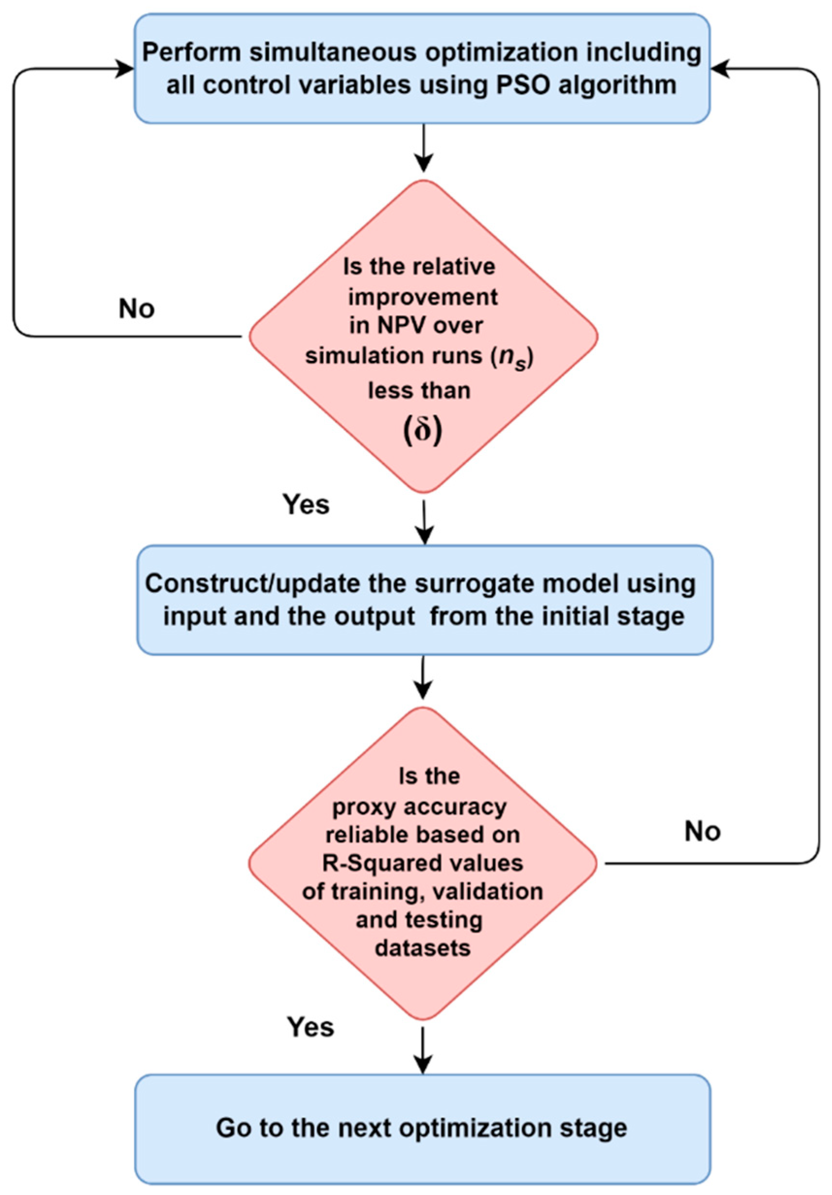
In this stage, the PSO algorithm is employed to conduct simultaneous optimization of all control variables, providing an initial exploration of the search space. The PSO global search capability makes it a suitable choice for this initial optimization stage to explore the search space and identify promising regions. The data generated during this initial optimization stage are also used to construct and update a proxy model based on the RBF artificial neural network. The developed online proxy model is iteratively updated to ensure it mimics the global performance of the objective function with reasonable accuracy. This approach is found to provide superior performance as compared to the offline sampling techniques [53]. Note that the proxy is only used for sensitivity analysis as explained in the next section. As shown in Figure 4, the initial stage is terminated when both of the following criteria are met:
(1)
The relative improvement ( I r ) in the objective function over a specified number of simulation runs ( n s ) is less than a threshold value ( δ ) [28,54]. The relative improvement is calculated using Equation (16).
I r = J 2 J 1 J 1 × 100
where J 2 is the current objective function at which we calculate the relative improvement; J 1 is a previous objective function located at ( n s ) simulation runs before the current objective function. In this work, n s = 500 and δ = 1% are used to calculate the relative improvement in the objective function.
(2)
The proxy model achieves a reasonable accuracy calculated based on the R-squared values for the training, validation, and testing sets using Equation (17):
R 2 = 1 S S E S S T = 1 i = 1 n J i a c t J i p r o x y 2 i = 1 n J i a c t J i a c t ¯ 2
where S S E and S S T represent the sum of square error and the sum of total error, respectively. J i a c t and J i p r o x y are the objective functions (NPVs) obtained from the actual reservoir model and proxy model, respectively. J i a c t ¯ are the average objective function values obtained from the simulator and n is the size of the training, validation, and testing sets.
The two criteria ensure that the proxy model provides a reasonable global prediction performance while performing an initial exploration of the search space.

3.2. Enhanced Optimization Stage

In the enhanced optimization stage (Figure 5), the VARS method is applied to the verified proxy model from the initial optimization stage, to explore the relationship between the control variables (FCD settings) and the objective function. The proxy model facilitates the extensive global sensitivity calculations, which require evaluating the objective function (NPV) by varying the input parameter values numerous times (ranging from thousands to millions) to truly assess sensitivities. The proxy model accomplishes this by mimicking the behaviour of the resource-intensive numerical reservoir model, leading to substantial reductions in computational expenses.
Subsequently, the control variables are ranked and divided into two groups (the high and low-impact groups) based on their total variogram effects or indices (i.e., IVARS50) obtained from VARS analysis. The high-impact parameters group is characterized by high total effects, indicating that these parameters have the greatest impact on the objective function so that any small changes in their values can lead to significant changes in the objection function. This group also represents a minor proportion of the overall count of control variables and exhibits a relatively high level of independence due to their limited interaction effects. The low-impact group, on the other hand, is characterized by low main value effects with total effects also being influenced by the interaction between the control variables, indicating a relatively low direct impact of these parameters on the objective function.
Previous work by Ahdeema et al. [28] showed that a degraded optimization performance can be observed when high-impact parameters are distant from their optimal or near-optimal values. Thus, an enhanced optimization performance can be achieved by concentrating the optimization effort on the most influential (high impact) parameters followed by optimizing the rest of the parameters (low impact), using fit-for-purpose optimization algorithms.
The high-impact parameters are optimized first using the PSO algorithm, recognized for its global optimization capability and effective performance in problems with a low number of control variables, while the low-impact group remains fixed at their optimized values from the initial stage. The process continues until a predefined number of simulation runs is reached. Subsequently, the low-impact group undergoes optimization using the SPSA algorithm to refine the solution obtained from the high-impact group optimization. Given that the low-impact group encompasses a larger set of control variables, it provides an appropriate context for optimization through gradient-based algorithms such as SPSA, as indicated by [55]. Furthermore, the outcome obtained from optimizing the high-impact group serves as a good starting point for optimizing the low-impact group.

4. Case Study—Olympus Model

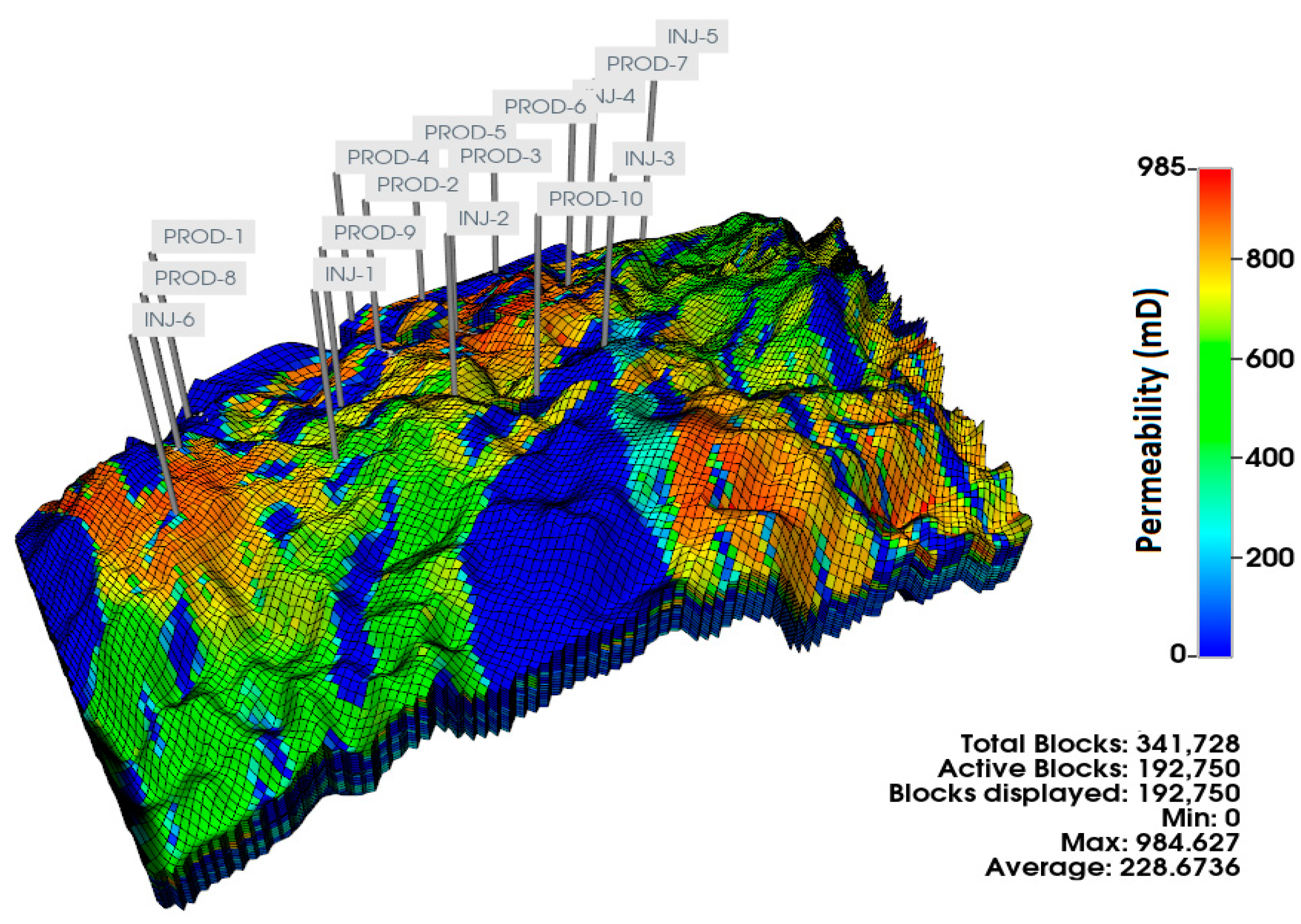
The Olympus was developed as a benchmark model for assessing well control and field development optimization in the North Sea environment [56]. The field covers a 9 × 3 km area with a boundary fault and minor faults in the reservoir. The model comprises 341,728 grid cells and 16 layers, with an impermeable shale layer separating it into two reservoirs: an upper reservoir with high-permeable channel sands integrated with floodplain shales, and a lower reservoir with less heterogeneity and coarser, medium, and finer grain size sands. The reference model includes 10 producers and 6 injectors operated based on pressure constraints as shown in Figure 6. Uncertainty in the reservoir was captured through the creation of an ensemble of 50 realizations with the porosity, permeability, net-to-gross, and initial water saturation considered as uncertain parameters. The ensemble of models was created through the following process: Initially, a high-fidelity base model consisting of around 5 million grid cells was generated. Subsequently, five wells were drilled into this base model, and synthetic logs were produced for each of these wells. These logs were subsequently employed to constrain the development of a set of 50 high-fidelity models aimed at capturing uncertainty.
For the hybrid optimization workflow demonstration, we utilize a deterministic optimization approach employing a single geological realization. Although the HO framework can be extended to account for geological uncertainty using multiple realizations (i.e., robust optimization), this particular approach is outside the scope of this paper. In this study, we use and modify realization 22 by developing it with 3 intelligent dual-lateral wells instead of 10 conventional producers, where top laterals target the top reservoir and bottom laterals target the bottom reservoir. Figure 7 shows the permeability distribution in each layer in realization 22, including the locations of producers and injectors. All wells produce under the maximum liquid rate of 3000 m3/day and minimum bottom hole pressure of 138 bar constraints. The injector wells operate at the maximum bottom hole pressure of 235 bar and the maximum injection rate of 1600 m3/day. The laterals are divided into multiple production zones using production packers based on the permeability profiles, with ICDs in each zone resulting in 26 equivalents (i.e., zone-representative) ICD design variables. Interval control valves are used at the lateral junctions (i.e., 6 ICVs in total) controlled proactively over six months for 10 years of production resulting in 120 control variables (146 control variables in total). Equivalent ICD settings range from 0.001 to 1 where 0.001 and 1 reflect very restrictive and almost no restriction, respectively, while ICV settings range from 0 to 1 where the upper and lower bounds indicate shut-in and fully open modes for the ICV. The ICD control variables are designated with the well name (W1, W2, or W3) and the lateral name (L1 or L2) followed by the ICD number (D1, D2, etc.). For example, W1L2D3 indicates the ICD located in zone 3 of the bottom lateral in well 1. The control variables for ICVs are indicated using well numbers and valve names where V1 is top and V2 is bottom, followed by the timestep. For instance, W2V1T3 refers to the top branch valve in well 2 at timestep 3.
The objective is to maximize the NPV by dynamically optimizing the settings of multiple types of flow control devices using a limited budget of 2500 simulation runs. The fluid flow is modelled using iSegWellTM [35] where the well is divided into multiple compartments and pressure drop is calculated using the multisegmented well model [57]. Pressure drops across ICDs and ICVs are controlled by adjusting the pressure loss multipliers instead of changing the flow area directly.
Figure 8 shows the initial optimization phase of the HO framework utilizing the PSO algorithm. This phase terminates at 1670 simulation runs, meeting the two subsequent termination conditions, as explained in Section 3.1. The first criterion is fulfilled when the relative enhancement ( I r ) in the objective function falls below the predefined threshold ( δ ) of 1% to 0.82% based on Equation (16). This occurred specifically between 1170 and 1670 simulation runs at corresponding NPVs of J 1 = 1.81 × 10⁹ and J 2 = 1.825 × 10⁹, respectively. This implies that the PSO optimization has reached convergence, suggesting further optimization is unlikely to provide significant improvements. The collected data from this initial optimization stage is split into three sets: a training set with 1350 samples, a validation set with 150 samples, and a testing set with 170 samples. The second termination criterion is met as the R-squared values for the training, validation, and testing sets become close to one with 0.99, 0.93, and 0.95, respectively, as shown in Figure 8. It should be noted that during this stage, the PSO population size is set as 80 for demonstration purposes. However, the choice of the population size is not very critical for this initial global exploration stage, as the subsequent enhanced optimization stage provides a refined search.
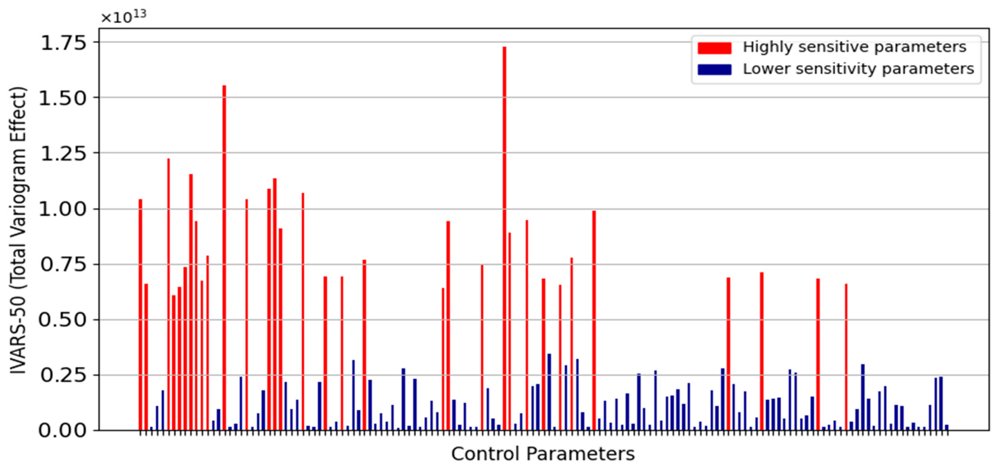
The VARS analysis is then carried out on all 146 control variables using the validated and tested RBF-based proxy model from the initial stage. The control variables are then classified into high-impact and low-impact groups based on their total variogram effects (IVARS50s), (Figure 9). Table 2 shows 33 high-impact parameters that were obtained from the VARS analysis.
As mentioned earlier, the parameters of the high-impact group play a crucial role in optimization, as they are highly sensitive. Even a slight alteration in their ranges can result in a significant change in the objective function value. To mitigate the adverse effects caused by these parameters when their values deviate from the near-optimal settings, a brief focused simulation run using PSO is performed on the high-impact group’s parameters, while keeping the parameters of the low-impact group fixed to their best values from the initial stage. The number of simulation runs or iterations needed to optimize this particular group depends on the observed relative improvement in the objective function. If the relative improvement is slow, it suggests that most of the highly sensitive parameters are already close to their optimal values and fewer simulation runs are required for optimizing this group. The number of parameters in this group is also a crucial factor in determining the required number of simulation runs. As the high-impact group has a small number of parameters compared to the total number of control variables, it typically requires fewer simulation runs with a smaller population size to allow the algorithm to converge. Additionally, the remaining simulation budget after the initial stage becomes an important factor at this point. If the criteria for terminating the initial stage are met late, the user must carefully allocate the remaining simulation runs. It is essential to ensure that there are enough simulation runs dedicated to optimizing both the parameters with high impact and those with low impact. Taking consideration of the previous discussion, it was decided to allocate 300 simulation runs for the high-impact group optimization using PSO with a population size of 20 to allow a more efficient algorithm performance.
When the switching criterion is satisfied, the SPSA algorithm is utilized to optimize the low-impact group, while high-impact parameters are fixed at their best values obtained from the PSO optimization of the high-impact group. The SPSA performance relies on its tuning parameters (i.e., step size α k , perturbation size c k , and number of perturbations); therefore, sensitivity analysis was performed on a and c , where a = 2 and c = 0.5 were found to provide the stable performance of SPSA.
Figure 10 shows the hybrid optimization (HO) performance during the optimization process, where the initial optimization stage is labelled with a solid black line. The high-impact group optimization using the PSO algorithm is represented by a solid red line. The solid green indicates the optimization of the low-impact group using the SPSA algorithm. The results show that the hybrid optimization framework was successful in achieving superior performance with a USD 1.94 billion NPV compared to the standalone PSO (dashed black line) with USD 1.83 billion, resulting in, approximately, a 6% increase in NPV or USD 110 million increase in profits. The HO takes advantage of a fit-for-purpose combination of optimization techniques to better explore the search space and provide a refined search in promising regions. The optimization process targeting high-impact parameters successfully redirected the search for the optimal solution, guiding it towards a more favorable position within the search space. Nevertheless, the extent of this shift is contingent upon the initial distance of the high-impact parameters from their optimal values. It is noteworthy how the low-impact optimization produced a more substantial incremental increase in Net Present Value (NPV) compared to its high-impact counterpart. This phenomenon can be attributed to the cumulative effect of the numerous low-impact variables, each of which may individually exert a modest influence. In contrast to the high-impact parameters, the sheer quantity of low-impact variables contributes significantly to achieving a comparable NPV enhancement.
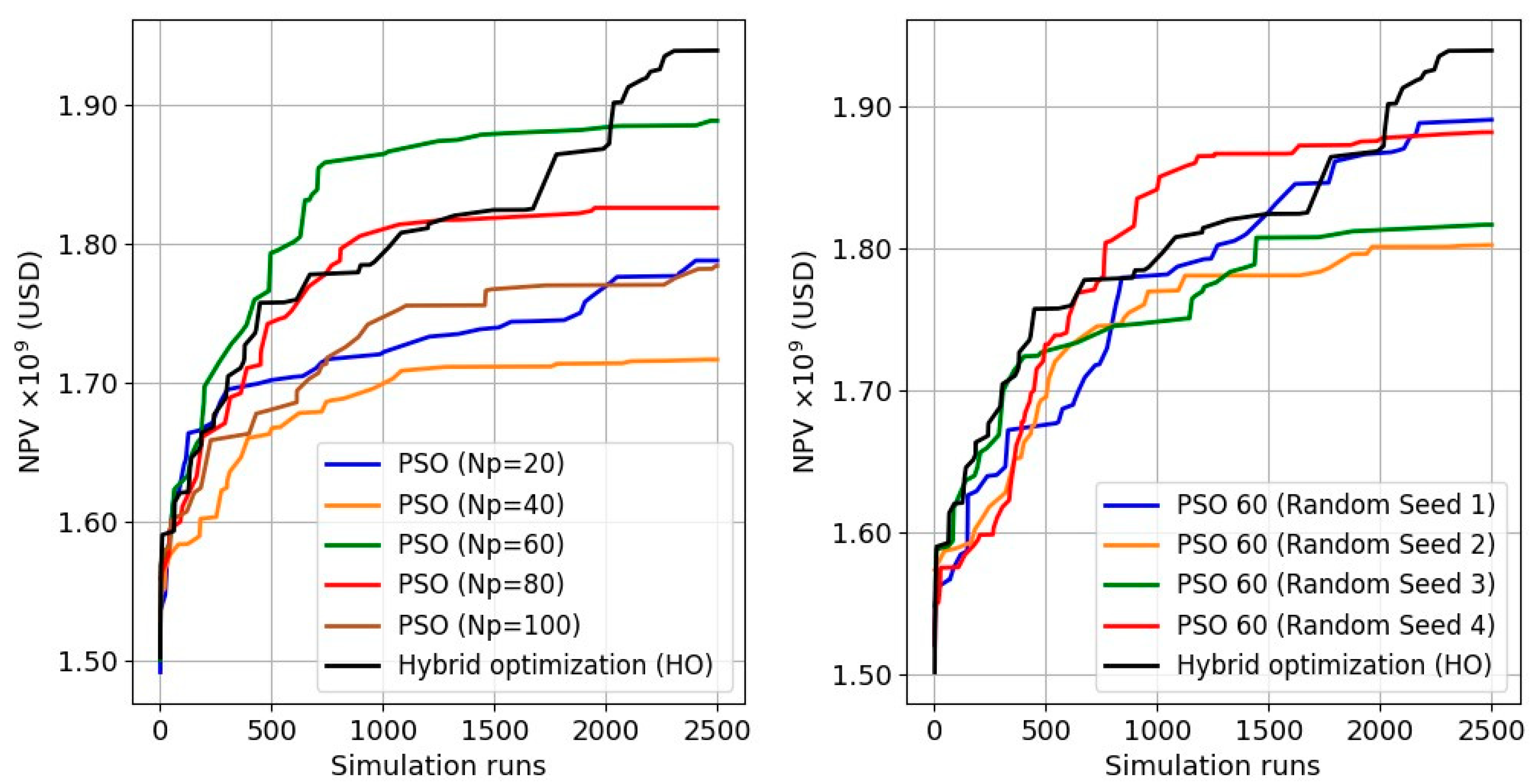
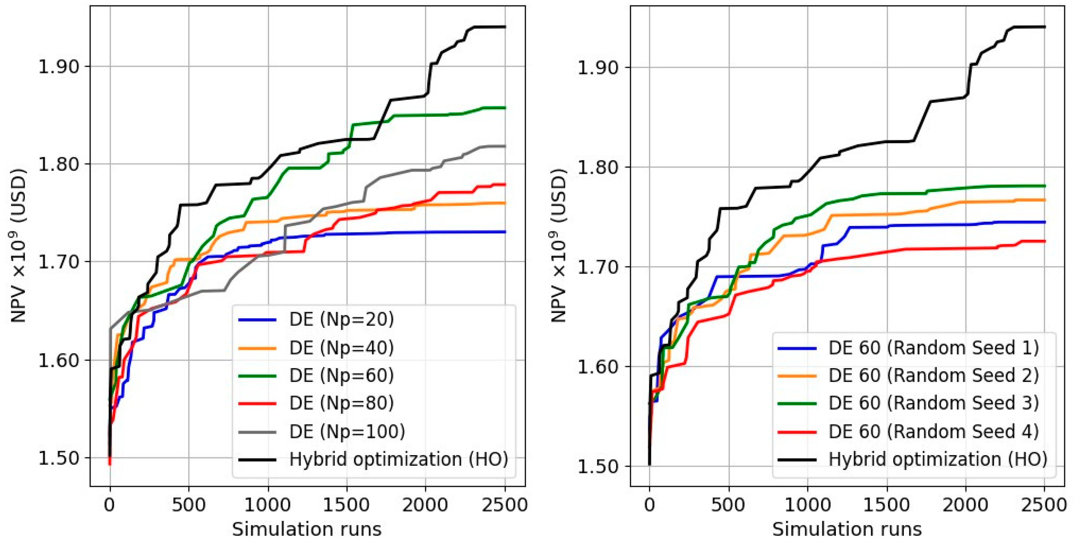
The performance of the HO was compared with the popular metaheuristic optimization algorithm, PSO and DE (differential evolution algorithm) [58]. Due to the inherent randomness of the population-based algorithms, the PSO and DE were tested with multiple population sizes and different random seeds (Figure 11 and Figure 12).
In all cases, HO succeeded in achieving better final results as compared to the population-based algorithms. PSO and DE ultimately fail to converge to an optimal solution due to the lower performance of metaheuristic algorithms with a large number of control variables. HO, on the other hand, takes advantage of the initial exploration of the search space provided by a metaheuristic algorithm (PSO), followed by a more refined search in promising regions using a combination of metaheuristic (PSO) and gradient-based (SPSA) algorithms for high-impact and low-impact variables, respectively.
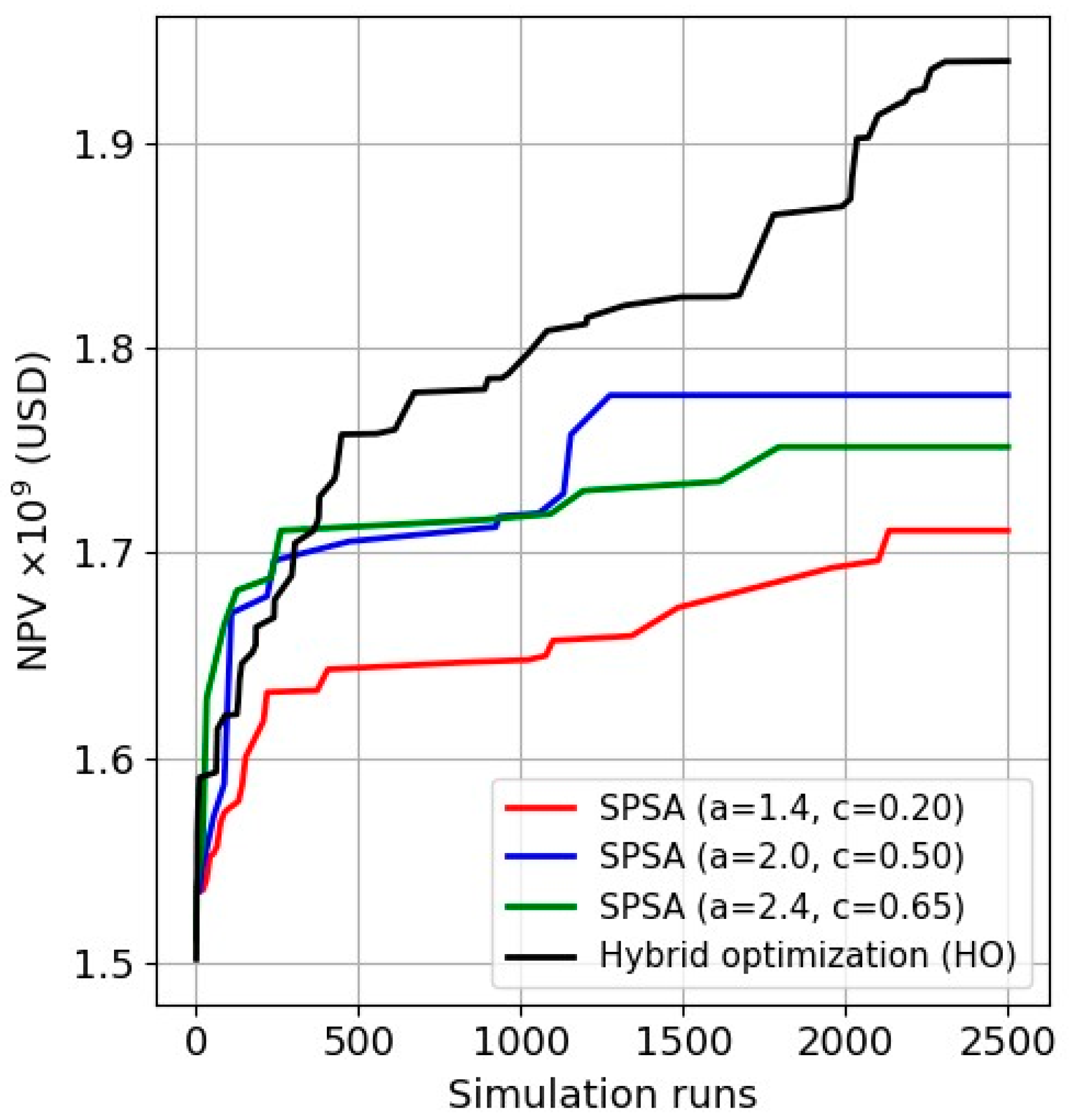
We also compared the optimization performance of HO with the SPSA algorithm using multiple tuning parameters (i.e., a and c ). The HO still provides a better solution, as shown in Figure 13, as SPSA often struggles to achieve convergence to a nearly optimal solution, primarily due to its susceptibility to becoming trapped in local optima.
Additionally, the efficiency of HO was compared with an industry-standard sequential optimization approach [59] using PSO, DE, and SPSA algorithms, Figure 14. In this optimization technique, the input parameters are divided into two groups based on their type and optimized sequentially in two stages. In the first stage, ICD control variables undergo optimization, while ICVs are held at their fully open setting. This stage continues until no significant improvement is observed in the objective function (i.e., after about 1000 simulation runs). In the second stage, the ICV control variables undergo optimization, while ICD control variables are held fixed at their optimum values obtained in the first stage. Sensitivity analyses were performed to determine the population sizes for PSO and DE, and the best values were found to be 20 for the ICD’s optimization stage and 80 for the ICV’s optimization stage for both metaheuristic algorithms. SPSA was found to perform better with tuning parameters a = 2 and c = 0.5, while the number of perturbations was equal to 10 for both optimization stages.
The HO outperforms the sequential optimization methods. This indicates that optimizing parameters separately based on their type without taking into account the correlation and interaction between them can result in poor simulation performance.
Table 3 provides a comprehensive overview of the optimal solutions achieved through various optimization techniques employed in this study, highlighting their performance in terms of cumulative oil, cumulative water, NPV, and incremental change in NPV. With a USD 1.94 billion profit and a 26.37% increase in NPV over the base case, HO exhibits the most significant improvement. It is worth emphasizing that the NPVs listed in Table 3 represent the best results achieved by each standard optimization algorithm. It is important to note that these algorithms might not deliver high-performance results consistently. For instance, the PSO algorithm generated relatively low solution NPVs ranging between USD 1.72 billion and USD 1.89 billion, as indicated in Figure 11. This variability can be attributed to the stochastic nature of the PSO algorithm, factors such as population size, and the quality of the initial population. In its best-case scenario, the PSO “got lucky” and achieved a high NPV, with a 23.04% increase in the NPV, which is approximately 3% lower than the one obtained from the hybrid optimization technique (26.37%). However, a 3% difference achieved by HO still translates to a significant financial difference of USD 51 million. This difference arises from other algorithms’ inability to discover optimal settings within the limited simulation budget. Moreover, HO excels at reliably guiding the optimization process towards more promising areas, ultimately resulting in higher NPVs. This advantage holds true even when the initial optimization stage performance is lackluster.
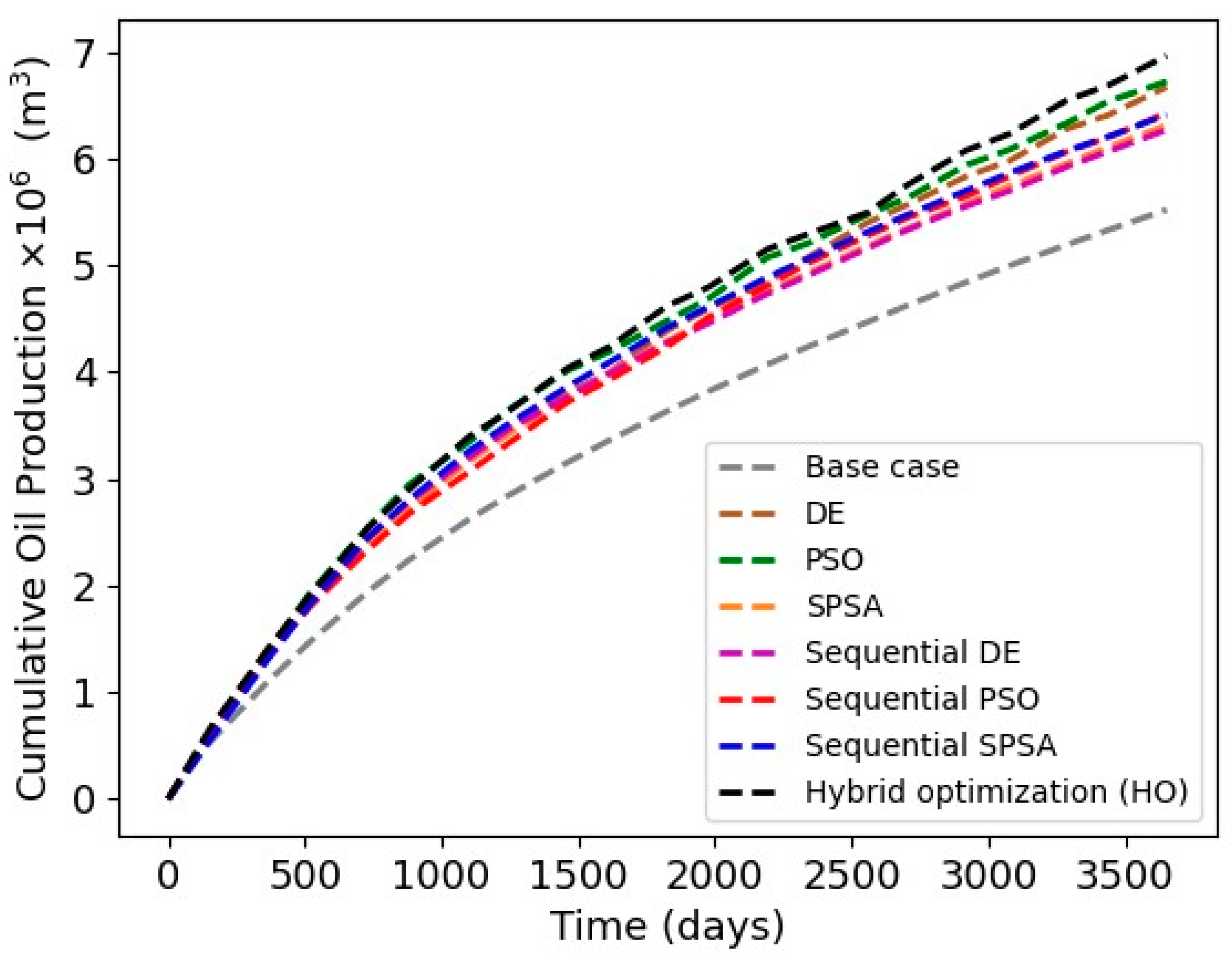
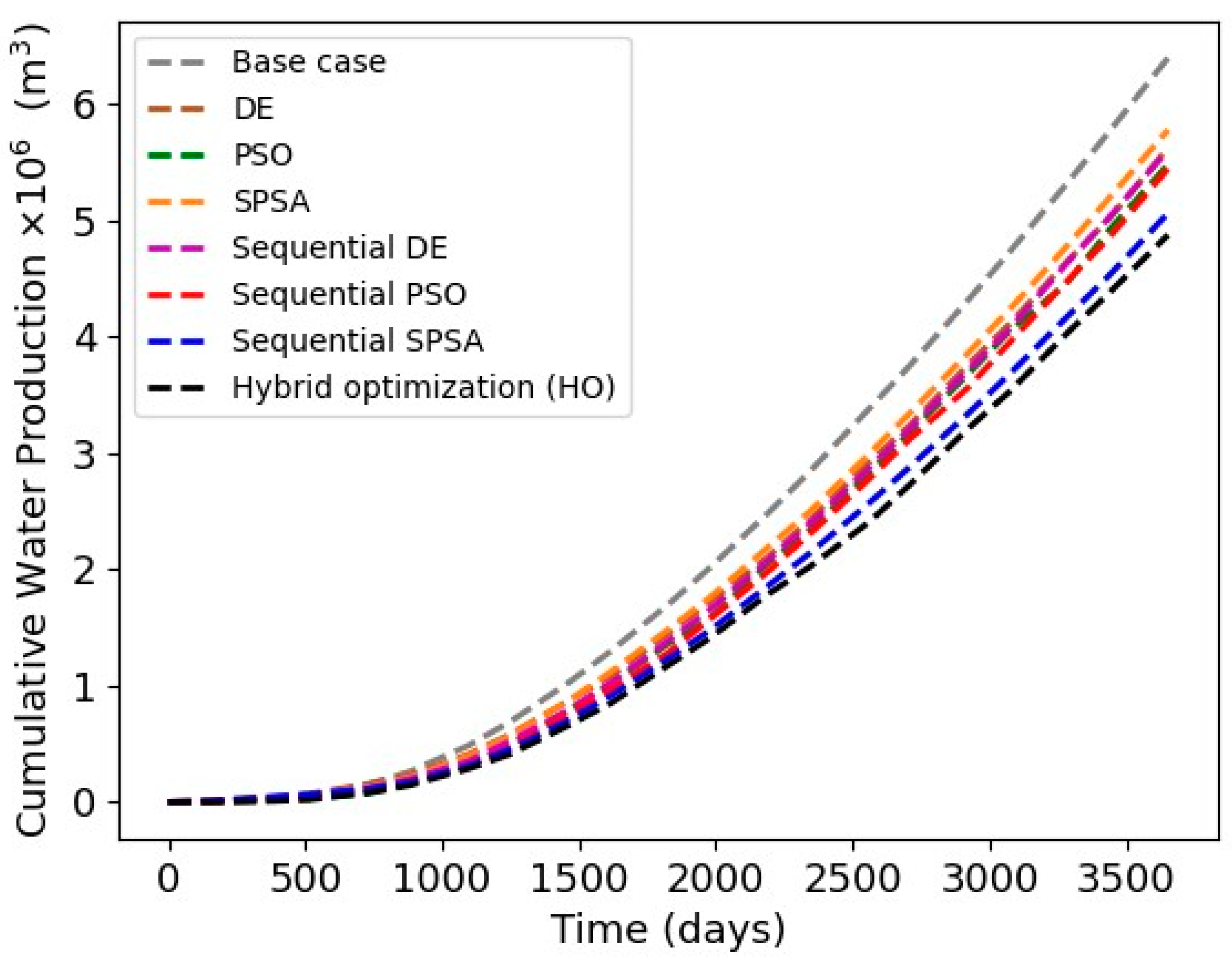
The increase in NPV achieved through HO is the result of a strategy that involves delaying water breakthrough in highly connected zones while simultaneously enabling higher oil production from other zones. This leads to a considerable decrease in the cumulative water production within the reservoir and an improvement in the reservoir’s cumulative oil production, as shown in both Figure 15 and Figure 16.
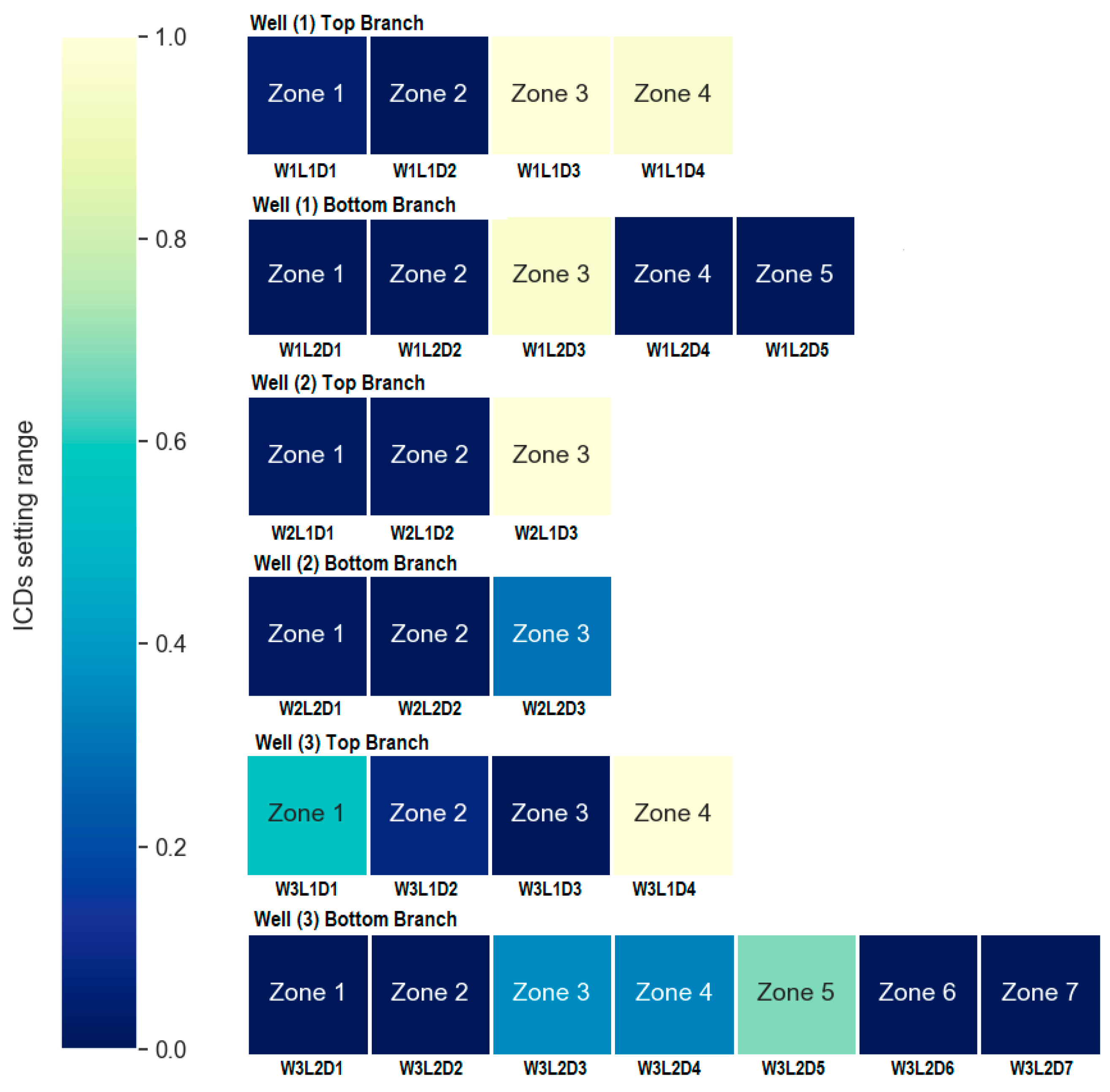
Figure 17 presents the final ICD setting map corresponding to the best (optimal) solution attained through the employment of the HO technique. The optimal control strategy was accomplished by allocating reduced ICD settings in zones where water intrusion occurs early, while less restrictive ICDs were allocated to other zones. For example, in the top lateral in well 1 (W1), ICD settings are very restrictive in zones 1 and 2 (W1L1D1 and W1L1D2), as these zones produce higher amounts of water than zones 3 and 4, where ICD settings are less restrictive (W1L1D3 and W1L1D4). This strategy enabled efficient water control while increasing oil production.
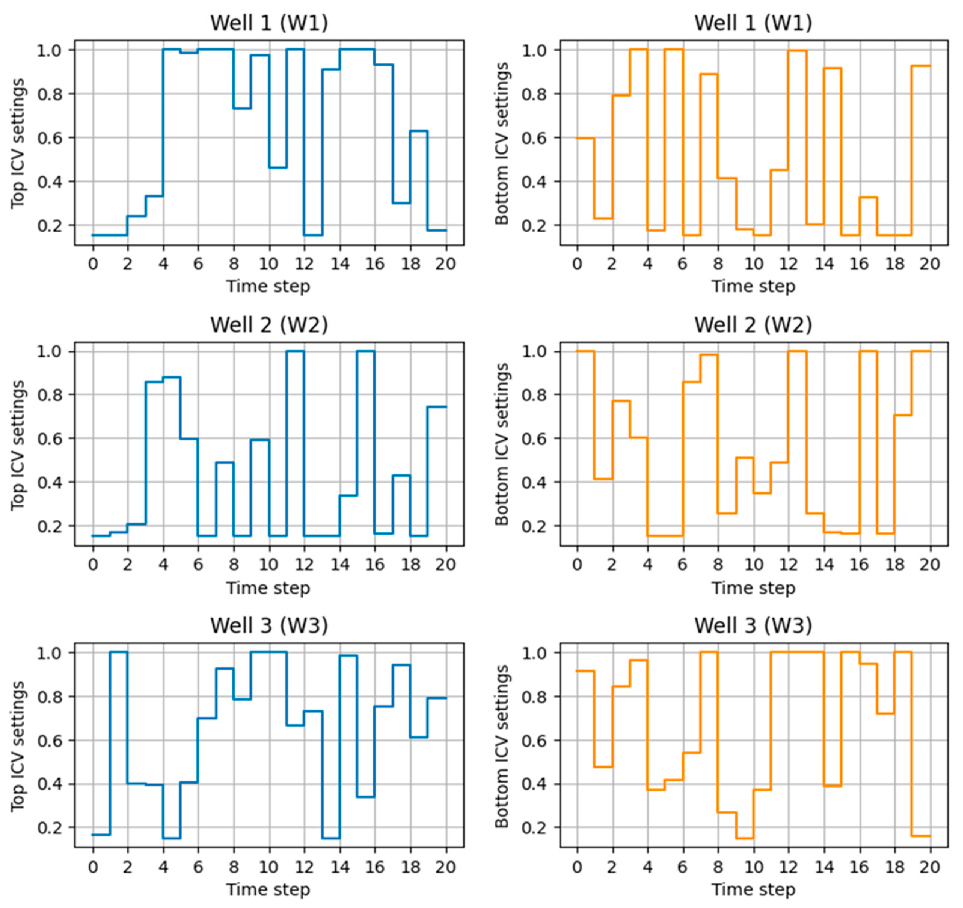
The ICVs, on the other hand, were alternately controlled to ensure that water production per branch was minimized while still satisfying operational constraints (Figure 18). This alternating behaviour of the ICVs is expected when the ICVs are controlled proactively (i.e., based on time rather than water cut). The ICVs’ behaviour ensured that all well branches contributed to production while proactively delaying the onset of water breakthrough in each branch.

5. Conclusions

In this work, we developed a multistage hybrid optimization framework to enhance the dynamic optimization process of intelligent completion design in multilateral wells with multiple types of flow control devices. The hybrid optimization framework aims to enhance the optimization performance by simplifying the problem and prioritizing the optimization process based on the expected impact of the parameters. In the first stage, the PSO algorithm is used to perform simultaneous optimization, while the generated input and output data are used to build a proxy model. In the second stage, the control variables are categorized into two groups (high- and low-impact groups) using VARS with the aid of the proxy model. Furthermore, the high-impact group was optimized first using PSO followed by optimizing of the low-impact group using SPSA.
The hybrid optimization framework was applied to Olympus, a benchmark reservoir model developed by three dual-lateral wells completed with ICDs across the laterals and ICVs at the junctions. The suggested hybrid optimization techniques were compared to standard optimization algorithms (i.e., PSO, DE, and SPSA) and sequential optimization techniques. The results showed that the proposed hybrid optimization technique outperformed all standard and sequential optimization techniques, delivering approximately a 26.37% increase in the objective function and achieving an NPV of USD 1.94 billion. This success was achieved through improved water management by allocating restrictive ICD settings in highly permeable zones where early breakthrough is expected, while more tolerant ICD settings were allocated to other zones to allow for greater oil production. The ICVs were alternately controlled to ensure that water production per branch was at a minimum level. This strategy resulted in a reduction in water production from 6.4 to 4.87 million cubic meters (a 24% reduction in water) and an increase in oil production by 26%, reaching a cumulative 6.96 million cubic meters compared to the base case of 5.52 million cubic meters.

Author Contributions

J.A.: Conceptualization, methodology, coding, modelling, data analysis, and writing the manuscript. M.H.S.: Supervision, conceptualization, review/edit manuscript. K.M.: Supervision, review/edit manuscript. All authors have read and agreed to the published version of the manuscript.

Funding

This research was funded by the Libyan Ministry of Higher Education and Scientific Research (No. 1015-2019).

Data Availability Statement

Not applicable.

Acknowledgments

Authors are thankful to the sponsor, the Libyan Ministry of Higher Education, for providing financial support, and to the Computer Modelling Group (CMG) for allowing academic access to its software.

Conflicts of Interest

The authors declare that they have no known competing financial interest or personal relationships that could have appeared to influence the work reported in this paper.

Abbreviations

AFCDAutonomous flow control device
AICDAutonomous inflow control device
AICVAutonomous interval control valve
DEDifferential evolution
FCDFlow control device
FDFluidic diode
GAGenetic algorithm
HOHybrid optimization
ICDInflow control device
ICVInterval control valve
IVARSIntegrated variogram across a range of scales
MADSMesh adaptive direct search
MLWMultilateral well
NPVNet Present Value
PSOParticle swarm optimization
RBFRadial basis function
RCPRate-controlled production
RMSERoot-mean-square error
SPSASimultaneous Perturbation Stochastic Approximation
SSEThe Sum of the Square Error
SSTThe Sum of the Total Error
STBStock Tank Barrels
USDUnited States Dollar
VARSVariogram Analysis of Response Surface
VNDVariable neighborhood descent

Nomenclature (In the Order of Appearance)

J Net Present Value
s Total number of simulation steps
r Cost of water treatment or price of oil
q Production or injection rate
t Time
b Discount factor
x Optimization variable (see Equation (2))
v Optimization variable’s velocity in PSO (see Equation (2))
ω Weights used in the PSO algorithm (see Equation (3))
α A step size used in the SPSA algorithm (see Equation (4))
g ^ An approximated in the SPSA algorithm (see Equation (4))
a A tuning parameter used in SPSA algorithm (see Equation (5))
c A tuning parameter used in SPSA algorithm (see Equation (5))
ϑ A parameter defined in Equation (6)
γ A parameter defined in Equation (6)
A A parameter defined in Equation (6)
w Weight of neuron (see Equation (11))
Gaussian density function (see Equation (11))
σ j Distance scaling parameter
V Variance
h Perturbation size
E Expectation
I r Relative improvement

References

  1. Rosi, G.A.; Zhu, D.; Gates, I.D.; Wang, J. Passive flow control devices—Well design and physics of their different flow regimes: A review. J. Pet. Sci. Eng. 2022, 218, 110999. [Google Scholar] [CrossRef]
  2. Eltaher, E.; Muradov, K.; Davies, D.; Grassick, P. Autonomous flow control device modelling and completion optimisation. J. Pet. Sci. Eng. 2019, 177, 995–1009. [Google Scholar] [CrossRef]
  3. Moradi, A.; Samani, N.A.; Kumara, A.S.; Moldestad, B.M.E. Evaluating the performance of advanced wells in heavy oil reservoirs under uncertainty in permeability parameters. Energy Rep. 2022, 8, 8605–8617. [Google Scholar] [CrossRef]
  4. Addiego-Guevara, E.A.; Jackson, M.D.; Giddins, M.A. Insurance Value of Intelligent Well Technology against Reservoir Uncertainty. In Improved Oil Recovery Symposium; SPE: Tulsa, OK, USA, 2008. [Google Scholar]
  5. Sampaio, M.A.; Barreto, C.E.A.G.; Schiozer, D.J. Proactive Control Valves of Producer and Injector Intelligent Wells under Economic Uncertainty. In Proceedings of the EAGE Annual Conference & Exhibition Incorporating SPE EuropEC, Copenhagen, Denmark, 4–7 June 2012. [Google Scholar]
  6. Sefat, M.H.; Muradov, K.; Davies, D. Field Management by Proactive Optimisation of Intelligent Wells-A Practical Approach. In Proceedings of the SPE Middle East Intelligent Energy Conference and Exhibition, Dubai, United Arab Emirates, 28–30 October 2013. [Google Scholar]
  7. Naus, M.M.J.J.; Dolle, N.; Jansen, J. Optimization of Commingled Production Using Infinitely Variable Inflow Control Valves. SPE Prod. Oper. 2006, 21, 293–301. [Google Scholar] [CrossRef]
  8. Emerick, A.A.; Cunha, R.; Portella, M. Production Optimization With Intelligent Wells. In Proceedings of the SPE Latin American and Caribbean Petroleum Engineering Conference, Buenos Aires, Argentina, 15–18 April 2007. [Google Scholar]
  9. Alghareeb, Z.M.; University, S.; Aramco, S.; Horne, R.N.; Yuen, B.B.; Shenawi, S.H. Proactive Optimization of Oil Recovery in Multilateral Wells Using Real Time Production Data. In Proceedings of the SPE Annual Technical Conference and Exhibition, New Orleans, LA, USA, 4–7 October 2009. [Google Scholar]
  10. Almeida, L.F.; Vellasco, M.M.B.R.; Pacheco, M.A.C. Optimization system for valve control in intelligent wells under uncertainties. J. Pet. Sci. Eng. 2010, 73, 129–140. [Google Scholar] [CrossRef]
  11. Grebenkin, I.M.; Davies, D.R. A Novel Optimisation Algorithm for Inflow Control Valve Management. In Proceedings of the EAGE Annual Conference and Exhibition Incorporating SPE EuropEC, Copenhagen, Denmark, 4–7 June 2012. [Google Scholar]
  12. Asadollahi, M.; Nævdal, G.; Dadashpour, M.; Kleppe, J. Production optimization using derivative free methods applied to Brugge field case. J. Pet. Sci. Eng. 2014, 114, 22–37. [Google Scholar] [CrossRef]
  13. Augusto, M.; Pinto, S. Short-Term and Long-Term Optimizations for Reservoir Management with Intelligent Wells. In Proceedings of the SPE Latin American and Caribbean Petroleum Engineering Conference, Quito, Ecuador, 18–20 November 2015. [Google Scholar]
  14. Vasper, A.; Endre, J.; Mjos, S.; Thi, T.; Duong, T. Efficient Optimization Strategies for Developing Intelligent Well Business Cases. In Proceedings of the SPE Intelligent Energy International Conference and Exhibition, Aberdeen, UK, 6–8 September 2016. [Google Scholar]
  15. Botechia, V.E.; Araújo de Lemos, R.; Hohendorff Filho JC von Schiozer, D.J. Well and ICV management in a carbonate reservoir with high gas content. J. Pet. Sci. Eng. 2021, 200, 108345. [Google Scholar] [CrossRef]
  16. Farahi, M.M.M.; Ahmadi, M.; Dabir, B. Model-based water-flooding optimization using multi-objective approach for efficient reservoir management. J. Pet. Sci. Eng. 2021, 196, 107988. [Google Scholar] [CrossRef]
  17. Brouwer, D.; Jansen, J.; Intl, S.E. Dynamic Optimization of Waterflooding with Smart Wells Using Optimal Control Theory. SPE J. 2004, 9, 391–402. [Google Scholar] [CrossRef]
  18. Sarma, P.; Aziz, K.; Durlofsky, L.; Etc, C. Implementation of Adjoint Solution for Optimal Control of Smart Wells. In Proceedings of the SPE Reservoir Simulation Symposium, Houston, TX, USA, 31 January–2 February 2005. [Google Scholar]
  19. Zandvliet, M.J.; Handels, M.; Van Essen, G.M.; Brouwer, D.R.; Jansen, J.D. Adjoint-Based Well-Placement Optimization Under Production Constraints. SPE J. 2008, 13, 392–399. [Google Scholar] [CrossRef]
  20. Asadollahi, M.; Naevdal, G. Waterflooding Optimization Using Gradient Based Methods. In Proceedings of the SPE/EAGE Reservoir Characterization and Simulation Conference, Abu-Dhabi, United Arab Emirates, 19–21 October 2009. [Google Scholar]
  21. Dilib, F.A.; Jackson, M.D. Closed-Loop Feedback Control for Production Optimization of Intelligent Wells Under Uncertainty. SPE Prod. Oper. 2013, 28, 345–357. [Google Scholar] [CrossRef]
  22. Fonseca, R.M.; Leeuwenburgh, O.; Van Den Hof, P.M.J.; Jansen, J.D. Improving the ensemble-optimization method through covariance-matrix adaptation. SPE J. 2015, 20, 155–168. [Google Scholar] [CrossRef]
  23. Chen, B.; Reynolds, A.C. Optimal control of ICV’s and well operating conditions for the water-alternating-gas injection process. J. Pet. Sci. Eng. 2017, 149, 623–640. [Google Scholar] [CrossRef]
  24. Salehian, M.; Sefat, M.H.; Muradov, K. Development of a Multi-Solution Framework for Simultaneous Well Placement, Completion, and Control Optimization. In Proceedings of the SPE Europec featured at 82nd EAGE Conference and Exhibition, Amsterdam, The Netherlands, 18–21 October 2021. [Google Scholar]
  25. Sefat, M.H.; Muradov, K.M.; Davies, D.R. Optimal Field Development and Control Yields Accelerated, More Reliable, Production: A North Sea Case Study. In Proceedings of the SPE Intelligent Energy International Conference and Exhibition, Aberdeen, UK, 6–8 September 2016. [Google Scholar]
  26. Tympakianaki, A.; Koutsopoulos, H.N.; Jenelius, E. c-SPSA: Cluster-wise simultaneous perturbation stochastic approximation algorithm and its application to dynamic origin-destination matrix estimation. Transp. Res. Part. C Emerg. Technol. 2015, 55, 231–245. [Google Scholar] [CrossRef]
  27. Arouri, Y.; Sayyafzadeh, M. An accelerated gradient algorithm for well control optimization. J. Pet. Sci. Eng. 2020, 190, 106872. [Google Scholar] [CrossRef]
  28. Ahdeema, J.; Sefat, M.H.; Muradov, K. Hybrid Optimization Technique Allows Dynamic Completion Design and Control in Advanced Multilateral Wells with Multiple Types of Flow Control Devices. In Proceedings of the SPE Offshore Europe Conference and Exhibition, Aberdeen, UK, 5–8 September 2023. [Google Scholar]
  29. Mirzaei-Paiaman, A.; Santos, S.M.G.; Schiozer, D.J. Iterative sequential robust optimization of quantity and location of wells in field development under subsurface, operational and economic uncertainty. J. Pet. Sci. Eng. 2022, 218, 111005. [Google Scholar] [CrossRef]
  30. Yang, H.; Kim, J.; Choe, J. Field development optimization in mature oil reservoirs using a hybrid algorithm. J. Pet. Sci. Eng. 2017, 156, 41–50. [Google Scholar] [CrossRef]
  31. Fu, J.; Wen, X.H. Model-Based Multiobjective Optimization Methods for Efficient Management of Subsurface Flow. SPE Soc. Pet. Eng. J. 2017, 22, 1984–1998. [Google Scholar] [CrossRef]
  32. Ma, H.; Yu, G.; She, Y.; Gu, Y. A new hybrid production optimization algorithm for the combined CO2-cyclic solvent injection (CO2-CSI) and water/gas flooding in the post-CHOPS reservoirs. J. Pet. Sci. Eng. 2018, 170, 267–279. [Google Scholar] [CrossRef]
  33. Tozzo, E.; Cabral Seixas Costa, A.P.; Lins, I.D. A hybrid multi-objective genetic algorithm for scheduling heterogeneous workover rigs on onshore oil fields. J. Pet. Sci. Eng. 2020, 195, 107935. [Google Scholar] [CrossRef]
  34. Han, X.; Zhong, L.; Wang, X.; Liu, Y.; Wang, H. Well placement and control optimization of horizontal steamflooding wells using derivative-free algorithms. SPE Reserv. Eval. Eng. 2021, 24, 174–193. [Google Scholar] [CrossRef]
  35. CMG-IMEX, Computer Modelling Group Ltd.: Calgary, AB, Canada, 2022.
  36. Kennedy, J.; Eberhart, R. Particle Swarm Optimization. In Proceedings of the ICNN’95—International Conference on Neural Networks, Perth, WA, Australia, 27 November–1 December 1995; pp. 1942–1948. [Google Scholar]
  37. Clerc, M.; Kennedy, J. The Particle Swarm-Explosion, Stability, and Convergence in a Multidimensional Complex Space. IEEE Trans. Evolut. Comput. 2002, 6, 58–73. [Google Scholar] [CrossRef]
  38. Kim, J.; Lee, K.; Choe, J. Efficient and robust optimization for well patterns using a PSO algorithm with a CNN-based proxy model. J. Pet. Sci. Eng. 2021, 207, 109088. [Google Scholar] [CrossRef]
  39. Spall, J.C. Multivariate Stochastic Approximation Using a Simultaneous Perturbation Gradient Approximation. IEEE Trans. Autom. Contr. 1992, 37, 332–341. [Google Scholar] [CrossRef]
  40. Spall, J.C. An Overview of the Simultaneous Perturbation Method for Efficient Optimization. Johns. Hopkins APL Tech. Design. 1998, 19, 482–492. [Google Scholar]
  41. Salehian, M.; Sefat, M.H.; Muradov, K. A Multisolution Optimization Framework for Well Placement and Control. SPE Reserv. Eval. Eng. 2021, 24, 923–939. [Google Scholar] [CrossRef]
  42. Samuel, J.S.; Muggeridge, A.H. Fast modelling of gas reservoir performance with proper orthogonal decomposition based autoencoder and radial basis function non-intrusive reduced order models. J. Pet. Sci. Eng. 2022, 211, 110011. [Google Scholar] [CrossRef]
  43. Yu, H.; Xie, T.; Paszczyñski, S.; Wilamowski, B.M. Advantages of Radial Basis Function Networks for Dynamic System Design. IEEE Trans. Ind. Electron. 2011, 58, 5438–5450. [Google Scholar] [CrossRef]
  44. Taunk, K.; De, S.; Verma, S.; Swetapadma, A. A Brief Review of Nearest Neighbor Algorithm for Learning and Classification. In Proceedings of the 2019 International Conference on Intelligent Computing and Control Systems, ICCS 2019, Madurai, India, 15–17 May 2019; pp. 1255–1260. [Google Scholar]
  45. Marquardt, D.W. An Algorithm for Least-Square Estimation of Nonlinear Parameters. J. Soc. Indust. Appl. Math. 1963, 11, 431–441. [Google Scholar] [CrossRef]
  46. Razavi, S.; Gupta, H.V. A new framework for comprehensive, robust, and efficient global sensitivity analysis: 1. Theory. Water Resour. Res. 2016, 52, 423–439. [Google Scholar] [CrossRef]
  47. Morris, M.D. Factorial Sampling Plans for Preliminary Computational Experiments. Technometrics 1991, 33, 161–174. [Google Scholar] [CrossRef]
  48. Hamby, D.M. A Review of Techniques for Parameter Sensitivity Analysis of Environmental Models. Environ. Monit. Assess. 1994, 32, 135–154. [Google Scholar] [CrossRef] [PubMed]
  49. Sobol, I. Sensitivity Analysis for Nonlinear Model. Math. Model. Comput. Exp. 1993, 4, 407–414. [Google Scholar]
  50. Haghnegahdar, A.; Razavi, S. Insights into sensitivity analysis of Earth and environmental systems models: On the impact of parameter perturbation scale. Environ. Model. Softw. 2017, 95, 115–131. [Google Scholar] [CrossRef]
  51. Razavi, S.; Gupta, H.V. A multi-method Generalized Global Sensitivity Matrix approach to accounting for the dynamical nature of earth and environmental systems models. Environ. Model. Softw. 2019, 114, 1–11. [Google Scholar] [CrossRef]
  52. Do, N.C.; Razavi, S. Correlation Effects? A Major but Often Neglected Component in Sensitivity and Uncertainty Analysis. Water Resour. Res. 2020, 56, e2019WR025436. [Google Scholar] [CrossRef]
  53. Salehian, M.; Haghighat Sefat, M.; Muradov, K. Multi-solution well placement optimization using ensemble learning of surrogate models. J. Pet. Sci. Eng. 2022, 210, 110076. [Google Scholar] [CrossRef]
  54. Ma, Z.; Volkov, O.; Durlofsky, L.J. Multigroup strategy for well control optimization. J. Pet. Sci. Eng. 2022, 214, 110448. [Google Scholar] [CrossRef]
  55. Sefat, M.; Muradov, K.; Elsheikh, A. Proactive optimization of intelligent-well production using stochastic gradient-based algorithms. SPE Reserv. Eval. Eng. 2016, 19, 239–252. [Google Scholar] [CrossRef]
  56. Fonseca, R.M.; Della Rossa, E.; Emerick, A.A.; Hanea, R.G.; Jansen, J.D. Introduction to the special issue: Overview of OLYMPUS Optimization Benchmark Challenge. Comput. Geosci. 2020, 24, 1933–1941. [Google Scholar] [CrossRef]
  57. Holmes, J.; Barkve, T.; Hydro, A.S.A. Application of a Multisegment Well Model to Simulate Flow in Advanced Wells. In Proceedings of the SPE European Petroleum Conference, Hague, The Netherlands, 20–22 October 1998. [Google Scholar]
  58. Storn, R.; Price, K. Differential Evolution-A Simple and Efficient Heuristic for Global Optimization over Continuous Spaces. J. Glob. Optim. 1997, 11, 341–359. [Google Scholar] [CrossRef]
  59. Humphries, T.D.; Haynes, R.D.; James, L.A. Simultaneous and sequential approaches to joint optimization of well placement and control. Comput. Geosci. 2014, 18, 433–448. [Google Scholar] [CrossRef]
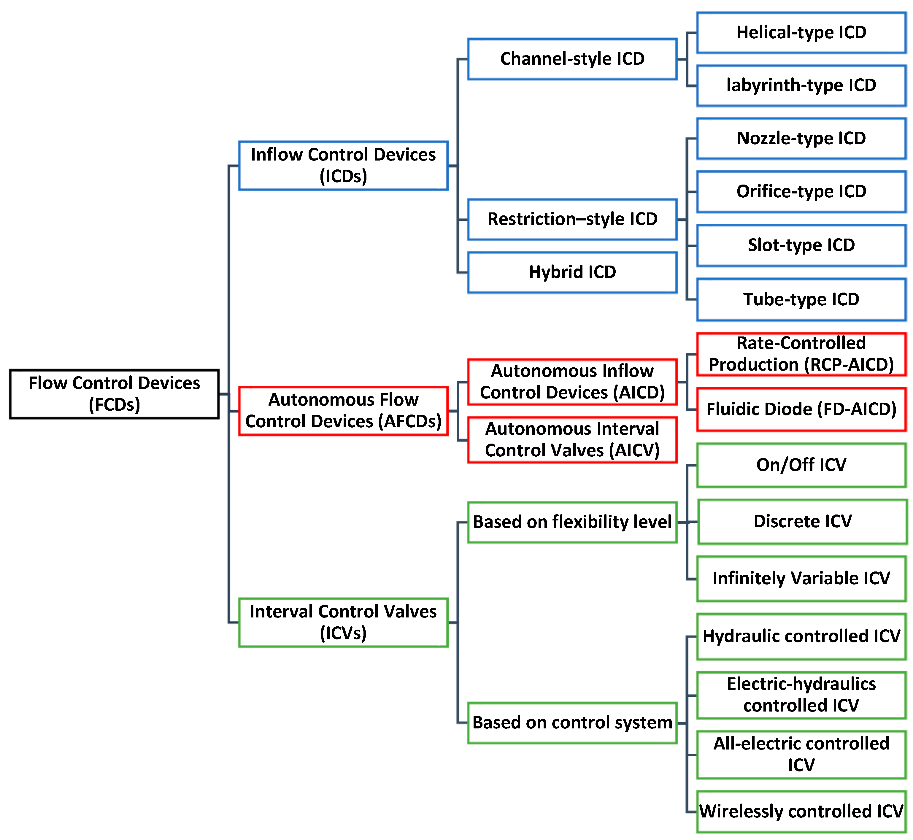
Figure 1. Types and classifications of flow control devices (FCDs).
Energies 16 07189 g001
Figure 2. Schematic of the velocity and position updates in the kth iteration in PSO [38].
Energies 16 07189 g002
Figure 3. Radial basis function architecture.
Energies 16 07189 g003
Figure 4. Initial optimization stage in the hybrid optimization (HO) framework.
Energies 16 07189 g004
Figure 5. Enhanced optimization stage in the hybrid optimization (HO) framework.
Energies 16 07189 g005
Figure 6. Top structure of the reference Olympus model.
Energies 16 07189 g006
Figure 7. Permeability distribution in X direction (PERMI) for all layers except layer 8 (shale) in the Olympus model (realization 22), showing the names (numbers) and locations of the producers (circles) and injectors (squares).
Energies 16 07189 g007
Figure 8. Initial optimization stage and proxy modelling training and validation: (a) objective function performance during initial optimization stage; (b) proxy model quality for training set (1350 experiments), (c) proxy model quality for validation set (150 experiments), (d) proxy model quality for testing set (170 experiments).
Energies 16 07189 g008
Figure 9. Total variogram effects (IVARS50s) for all 146 control variables.
Energies 16 07189 g009
Figure 10. The hybrid optimization performance during different stages and phases.
Energies 16 07189 g010
Figure 11. HO against standalone PSO algorithm applying different population sizes (left) and different seeds (right).
Energies 16 07189 g011
Figure 12. HO against standalone DE algorithm applying different population sizes (left) and different seeds (right).
Energies 16 07189 g012
Figure 13. HO against standalone SPSA algorithm.
Energies 16 07189 g013
Figure 14. HO against sequential optimization techniques based on PSO, DE, and SPSA.
Energies 16 07189 g014
Figure 15. Cumulative oil production of obtained optimal solutions from all optimization algorithms and techniques.
Energies 16 07189 g015
Figure 16. Cumulative water production of obtained optimal solutions from all optimization algorithms and techniques.
Energies 16 07189 g016
Figure 17. ICD settings map for hybrid optimization technique.
Energies 16 07189 g017
Figure 18. ICV settings during the field production life were obtained from the hybrid optimization technique.
Energies 16 07189 g018
Table 1. Economic parameters used in the optimization process.
ParameterField UnitsSI Units
Oil   price   ( r o )60 USD/STB377.39 USD/m3
Water   handling   cost   ( r p w )6 USD/STB37.74 USD/m3
Water   injection   cost   ( c w i )3 USD/STB18.87 USD/m3
Discount   rate   ( b )12%/year12%/year
Table 2. List of the high-impact parameters in the optimization problem based on total variogram effects.
High Impact Group (33 Highly Sensitive Parameters) Ranked Based on Their Appearance in the IVARSs Plot in Figure 9 from Left to Right
W1L1D2, W1L1D3, W1L2D3, W1L2D4, W1L2D5, W2L1D1, W2L1D2, W2L1D3, W2L2D1, W2L2D2, W3L1D2, W3L2D2, W3L2D6, W3L2D7, W1V1T01, W1V1T03, W1V1T05, W1V2T06, W1V2T08, W1V2T15, W1V1T16, W1V1T19, W2V1T01, W2V2T01, W2V1T03, W2V2T04, W2V1T06, W2V1T07, W2V1T09, W3V1T01, W3V1T04, W3V1T09 and W3V2T11
Table 3. Optimal solutions from all optimization algorithms and techniques in this study.
Algorithm/TechniqueCumulative Oil (m3) × 106Cumulative Water (m3) × 106NPV (USD) × 109NPV Increase Compared to the Base Case
Base case5.526.401.536-
Standard PSO6.725.471.89023.04%
Standard DE6.675.621.85720.90%
Standard SPSA6.315.771.77715.70%
Sequential PSO6.435.441.80017.19%
Sequential DE6.275.601.77115.30%
Sequential SPSA6.455.001.81618.23%
Hybrid optimization (HO)6.964.871.94126.37%
Disclaimer/Publisher’s Note: The statements, opinions and data contained in all publications are solely those of the individual author(s) and contributor(s) and not of MDPI and/or the editor(s). MDPI and/or the editor(s) disclaim responsibility for any injury to people or property resulting from any ideas, methods, instructions or products referred to in the content.