Article

Impact of Renewable and Non-Renewable Energy Consumption and CO2 Emissions on Economic Growth in the Visegrad Countries

by
Błażej Suproń
* and
Janusz Myszczyszyn
Department of Economics and Accounting, Faculty of Economics, West Pomeranian University of Technology, 70-310 Szczecin, Poland
*
Author to whom correspondence should be addressed.
Energies 2023, 16(20), 7163; https://doi.org/10.3390/en16207163
Submission received: 11 September 2023 / Revised: 16 October 2023 / Accepted: 18 October 2023 / Published: 19 October 2023
(This article belongs to the Section C: Energy Economics and Policy)

Abstract

:
This study presents empirical results regarding the relationships between renewable and non-renewable energy consumption, CO2 emissions, and the GDP within the Visegrád Group (V4) countries. Using FMOLS/DOLS and ARDL approaches, along with causality tests based on the Toda–Yamamoto method, this study explores these relationships at a regional level. The study fills the research gaps for a comprehensive analysis of the indicated relationships in the V4 countries by using both individual and panel models. The findings indicate that renewable energy has a small positive impact on long-term economic growth, with non-renewable energy having a more significant effect. Moreover, CO2 emissions have a negative impact on economic growth, suggesting an ongoing reliance on non-renewable energy sources and a burden on economic expansion. At an individual country level, the effects vary. Poland, Slovakia, and Hungary exhibit a negative relationship between CO2 emissions and economic growth. Energy sources also differ in regards to impact: in Poland, the Czech Republic, and Slovakia, non-renewable energy significantly affects economic growth, while in Hungary, renewable energy plays a more substantial role. Causality tests reveal a causal relationship between CO2 emissions and economic growth in the Czech Republic and Poland, suggesting that CO2 emissions significantly influence economic expansion. In terms of energy production, renewable energy is causally related to economic growth in the Czech Republic and Slovakia. All countries demonstrate significant causality between non-renewable energy and economic growth. Additionally, a relationship between renewable energy and CO2 emissions is confirmed in Poland.

1. Introduction

At a time of growing concern regarding climate change and ongoing sustainability policies, choosing between renewable and non-renewable energy sources has become a key decision for all countries worldwide. With the announcement of the Fit for 55 initiative in 2021, the Visegrad Group (V4) countries (the Czech Republic, Hungary, Poland, and Slovakia) face at a pivotal moment that will shape their energy landscapes and economic trajectories for the coming decades. Simultaneously, these countries serve as a pertinent example of regions grappling with important energy and environmental policy dilemmas, while at the same time, they have been building market-based economies for more than 30 years.
Against the backdrop of a shared history, after decades of communist rule, these countries have undergone a dynamic transformation, not only in terms of the economic landscape, but also in terms of energy paradigms. Despite significant investment in the energy infrastructure that these countries inherited from their communist history, it still lags behind Western European standards. This is because their energy system was, for many years, based on centralized energy production, with heavy reliance on non-renewable resources, as well as policies whose priorities often deviated from environmental sustainability. At the same time, energy demand was determined by the heavy industry that formed the backbone of their economies.
As the European Union (EU) increases its commitment to combating climate change and achieves ambitious greenhouse gas reduction targets, these countries are becoming both participants and observers in a monumental transformation. The Visegrad region, with its diverse landscapes and energy needs, is grappling with the overall need to reduce CO2 emissions while promoting economic growth and extensive investment in renewable energy. The energy transition will also require the V4 countries to increase the production of green electricity, which is expected to be the main source of energy in the future economy.
Considering this rationale, this study focuses on the impact of electricity consumption from renewable and non-renewable sources, as well as CO2 emissions, on economic growth in the Visegrad countries. Its genesis is based on considerations of, on the one hand, maintaining economic growth, which generates electricity demand, and, on the other hand, reducing its production from fossil fuels, which has a negative impact on the environment [1]. In this case, the recommended course of action is to increase the share of renewable energy in total energy production, which involves significant investment and expenditure. Secondly, due to the transition to a zero-carbon economy, electricity demand is increasing. For the V4 countries, this poses a significant challenge to increase electricity production while maintaining economic growth. This challenge is associated with the transition, such as the increased use of electric vehicles, the electrification of various sectors, and a shift away from fossil fuels to cleaner energy sources, all of which lead to a greater need for electricity.
This study aims to assess the impact of CO2 emissions and renewable and non-renewable energy consumption on economic growth in the V4 countries between 1991 and 2021. The study is designed to show both commonalities and individual differences between the group’s member countries. This approach is based on the theses proposed by Menegaki and Tsani [2], who pointed out that estimates for individual countries mostly differ from the results of pooled (panel) regression models, and that policy recommendations should be made at the national rather than regional or group level. Based on the stated objective and the literature review, the following research hypotheses were formulated.
H1. 
There is a positive and significant relationship between renewable energy consumption and economic growth in the individual Visegrad countries.
H2. 
There is a positive and significant relationship between non-renewable energy consumption and economic growth in the Visegrad countries.
H3. 
The increase in CO2 is negatively and significantly related to economic growth in the Visegrad countries.
H4. 
The relationship between renewable and non-renewable energy consumption and economic growth varies between the Visegrad countries.
To create these hypotheses, the study used panel methods such as fully modified ordinary least squares (FMOLS) and dynamic ordinary least square (DOLS) regression, as well as auto regressive distributed lag (ARDL).
This article attempts to make a scientific contribution in three areas: (1) the study of the dynamic relationship between the economic development of the V4 countries and renewable electricity production and CO2 emissions between 1991 and 2021; (2) a longitudinal analysis that allows conclusions to be drawn regarding the countries of the V4 Group of post-socialist countries, which underwent economic transitions in different ways after 1991 and which joined the European Union in 2004; (3) the use of modern econometric tools, i.e., dynamic panel data models, including the DOLS panel, the FMOLS panel and, a combination of the two, combined with individual analysis based on the ARDL model; the results obtained are important in the context of both academic considerations and decisions in the field of energy policy. The relationships between economic growth and renewable electricity consumption and production can serve as practical guidance for countries that are in the early stages of their energy transition. Econometric results from FMOLS, DOLS, and ARDL support and affirm the robustness of the regression model.
The following sections are included in the study. Section 2 presents the results of other studies regarding the link between energy, economic growth, and CO2 in EU and V4 countries. Section 3 describes the methodology, Section 4 presents the data using descriptive statistics, and Section 5 presents the empirical results, along with a discussion.
The article closes with conclusions, including policy implications arising from the research.

2. Literature Review

Studying the relationship between economic growth, energy consumption, and CO2 is the subject of many studies and a significant amount of research, whether in regards to individual countries, panel studies, or others.
At the current stage of economic development, including the dependence on non-renewable energy sources, in the face of conflicts, the exertion of influence by countries exporting non-renewable raw materials, as well as climate change and sustainability policies, it is important to study the impact of these factors on economic growth using a breakdown between non-renewable and renewable energy, with the inclusion of CO2.
From the literature review, it can be concluded that the nature of the relationship between energy consumption and economic growth falls into four theoretical paradigms: (1) the growth hypothesis (unidirectional causality: energy consumption affects economic growth), (2) the conservation hypothesis (economic growth is the cause of energy consumption), (3) the feedback hypothesis (bidirectional causality between economic growth and energy consumption), and (4) the neutrality hypothesis (no relationship) [3]. It should also be acknowledged that, initially, studies of relationships using econometric modeling focused on analyzing the level of economic growth versus total energy consumption, without disaggregating between renewable and non-renewable energy or the level of CO2 produced [4].
Marques et al., in their search for the relationship between energy consumption and the level of economic growth for the period 1968–2013, divided the different regions of the world into four areas: the Americas; Africa, Europe and Central Asia; Asia and the Pacific; and Africa and the Middle East. They confirmed the growth hypothesis for the countries of America, Africa, and the Middle East and the conservation hypothesis for Europe, Central Asia, Africa and the Middle East for this extended period. In the short term, bidirectional relationships were confirmed, except for in Africa and the Middle East [5].
For example, Huang, Hwang, and Yang, using World Bank panel data for 82 countries of the world for the period 1972–2002, looked for a relationship between economic growth and the level of energy consumption. The authors indicated that for the lower and upper-middle income group countries, economic growth positively influenced the level of energy consumption; for the high-income group countries, economic growth negatively influenced the level of energy consumption; while for the low-income group countries, no relationship was confirmed. In no case was it confirmed that the level of energy consumed influenced economic growth, which could have contributed to the reduction of non-renewable energy consumption and, therefore, the reduction of CO2, especially by the high GDP countries [6].
Alper and Oguz investigated the relationships between economic growth, renewable energy consumption, capital, and labor for the new EU member states between 1990 and 2009, using ARDL modeling, among other methods. A statistically significant causal relationship between renewable energy consumption and economic growth was confirmed for Bulgaria, Estonia, Poland, and Slovenia; only for the Czech Republic was economic growth the cause of renewable energy consumption [7].
Esso studied the long-run causal relationship between energy consumption and economic growth in seven sub-Saharan African countries, and using a co-integration model, his results confirm a unidirectional relationship between GDP and energy consumption levels in all the countries analyzed [8].
In turn, Fang, by analyzing data from 1978 to 2008, confirmed that for China, a 1% increase in renewable energy consumption increases real GDP by 0.12% [9]. Inglesi-Lotz, analyzing panel data for all of the OECD countries for the period from 1990 to 2010, confirmed the positive impact of renewable energy consumption on economic welfare [10].
Sebri and Ben-Salha used the ARDL model to investigate the relationship between economic growth, levels of renewable energy consumption, CO2 emissions, and trade openness for the BRICS (Brazil, Russia, India, China, South Africa) countries. The empirical results indicate a positive impact of renewable energy on the level of global production [11].
Bhattacharya et al. analyzed 38 top renewable energy-consuming countries, looking for the relationship between renewable and non-renewable energy consumption, capital and labor, and the output level between 1991 and 2012. The study confirmed that the level of renewable energy consumption had a positive impact on output for 57% of the countries in the sample [12].
Table 1 presents a synthetic overview of recent studies in which the authors have reflected Visegrad countries, providing an overview of the methods used to study the relationship between energy consumption, economic growth, and CO2.
It is important to note that there are no comprehensive studies regarding the relationship between renewable and non-renewable energy consumption, CO2 emissions, and economic growth in the Visegrad countries, according to the analysis of the existing literature and methodologies presented in Table 1. Although these countries have been included in similar studies involving a wider range of countries, the specificities of the region and individual economies have not been considered. However, our analysis of the existing literature suggests that previous studies have not simultaneously applied the ARDL, FMOLS, and DOLS methods, nor conducted causal analysis to obtain comprehensive and robust results. Therefore, this article aims to address these research gaps.
The Visegrad countries are significant because they represent a unique subset of Eastern and Central European nations that have undergone economic transitions in the post-communist era. These transitions have led to shifts in energy production and economic structures, making these countries an interesting case study for researchers and policymakers. The findings can help guide energy and environmental policies in these countries and contribute to a broader understanding of the relationship between energy, the environment, and economic growth. It is also important to consider similarities and differences, both at the regional level, using the FMOLS and DOLS models, and at local level, using the ARDL model.

3. Materials and Methods

3.1. Date

The article examines the relationship between renewable (REW) and non-renewable (NREW) energy consumption, carbon dioxide (CO2) emissions, and economic growth (GDP). The analysis was conducted for the V4 member countries from 1991 to 2021 (n = 31). As data have been recorded for all countries surveyed since 1991, all available and complete records from 1991 to 2021 are used. Null data did not occur in the series.
Electricity consumption was taken as gross electricity production expressed in tonnes of oil equivalent per capita, CO2 emissions were taken in metric tons per capita, and GDP was used as GDP per capita in constant 2015 US dollars. Data for GDP are from the World Bank’s WDI resource, while data for the NREW, REW, and CO2 variables come from the European Environment Agency database. Data were transformed into natural logarithms. Descriptive statistics for the time series studied are presented in Table 2.

3.2. Methodology and Econometric Framework

In order to represent the relationship between economic growth, renewable and non-renewable energy production, and CO2, and to isolate both joint and individual effects, two models were developed. A panel model was used to examine common features, while separate models were estimated for individual data. The overall research problem can be represented by the following mathematical equation:
Δ G D P t = f C O 2 , R E W , N R E W
The model was transformed to a log-linear form to eliminate serial correlation and heteroskedasticity, which is shown below:
l n G D P t = β 0 + β 1 t l n C O 2 t + β 2 t l n R E W t + β 3 t l n N R E W t + ε t
In the first stage of the study, tests of the stationarity of the variables were carried out through tests provided for both individual and panel data. For panel data, three different types of tests were used: the Pesaran test and the Shin IPS [31], the Levin, Lin, and Chu (LLC) test [32], and the second generation CIPS test (Cross-Sectionally Dependent Panel Unit Root Test) [33]. For individual testing, the Dickey–Fuller (ADF) [34] and the Phillips–Perron (PP) unit root tests [35] were used. The use of the two types of tests at both the individual and panel levels ensured the robustness of the results obtained.
Based on the results of the unit root tests, the co-integration of the panel and individual data was estimated in the study’s next step. Due to the relatively small cross-section of the panel, tests for panel data were applied according to the methods of Kao [36] and Pedroni [37]. For individual data, the ARDL boundary test was used, due to the length of the time series.
A form of the ARDL model that examines the long-term relationship between selected variables is shown below [38]:
Δ lnGDP t =   c   +   β 0 lnGDP   + i = 1 m β 1 i Δ lnGDP t i + i = 1 m β 2 i Δ lnCO 2 t i     + i = 1 m β 3 i Δ lnREW t i + i = 1 m β 4 i Δ lnNREW t i + δ 1 lnGDP t 1     +   δ 2 lnCO 2 +   δ 3 lnREW t 1 +   lnNREW t 1 +   ε t
where:
-
Δ represents the first difference value of the variable;
-
δ represents the long-term rate;
-
ε(t) represents the residual component.
In order to test the absence of a long-term relationship, the hypothesis H0: δ 1 = δ 2 = δ 3 = δ 4 and the alternative hypothesis H1: δ 1 δ 2 δ 3 δ 4 are used. If the calculated F-statistic is higher than the upper limit of the critical value I(1) for the number of explanatory variables (k), the null hypothesis will be rejected. If the F statistic is less than the lower limit of the critical value I(0), the null hypothesis cannot be rejected. An F statistic that is between I(0) and I(1) indicates an undecided co-integration [38].
After examining the co-integration when a long-run relationship was shown, the panel and individual models were estimated in the next step. A fully modified OLS (also known as FMOLS) [39], along with the dynamic ordinary least squares (DOLS) [40,41], was estimated for the panel data. FMOLS is a technique for performing the most efficient method of cointegrating regression analysis while negating endogeneity error and serial correlation. To confirm the consistency of the results, DOLS was estimated, which is specifically designed for cointegrated time series data and is well suited for estimating long-run relationships, especially in small panels. The panel analysis was designed to show the typical characteristics of the countries studied. The general form of the estimator used in the study is presented below [39]:
B ^ F P W = i = 1 N t = 1 T X ˜ i t * X ˜ i t * , 1 i = 1 N t = 1 T ( X ˜ i t * y ˜ i t * λ 12 i * )
When co-integration was demonstrated for the individual data, a different technique was used to estimate the relationship. In order to capture both the long-run relationship and the adjustment process in disequilibrium, a constrained error correction model (ECM), expressed in the following form, was used [42]:
Δ lnGDP t =   δ 0 + i = 0 p δ 1 i Δ lnGDP t i + i = 1 q 1 δ 2 i Δ lnCO t i + i = 1 q 2 δ 3 i Δ lnREW t i   + i = 1 q 3 δ 4 i Δ lnNREW t i + Φ E C M t 1 + ε t
where the ECM correction factor is determined from the residuals of the long-term model [43]:
lnGDP t = c +   δ 1 lnCO +   δ 2 lnREW   +   δ 3 lnNREW   +   ε t
In the final stage of the study, causality tests for individual data were conducted based on the Toda–Yamamoto (TY) test [44]. Using the S-VAR model, the T–Y method is performed in two steps. First, the optimal lag length and the maximum order of integration are determined, and then the VAR model is estimated at the series level. In addition, whether or not the model has been determined correctly is also tested. The MWALD technique is used to assess causality within the VAR model in the second stage (where k = p + dmax). In this research, we employ the T–Y procedure of the causality test by estimating the VAR models, as outlined below:
l n G D P t = α 1 + i = 1 p + d m a x β 1 i l n G D P t i + i = 1 p + d m a x γ 1 i l n C O 2 t i + i = 1 p + d m a x θ 1 i l n R E W t i + i = 1 p + d m a x π 1 i l n N R E W t i + ε 1 t
l n C O 2 t = α 2 + i = 1 p + d m a x β 2 i l n G D P t i + i = 1 p + d m a x γ 2 i l n C O 2 t i + i = 1 p + d m a x θ 2 i l n R E W t i + i = 1 p + d m a x π 2 i l n N R E W t i + ε 2 t
l n R E W t = α 3 + i = 1 p + d m a x β 3 i l n G D P t i + i = 1 p + d m a x γ 3 i l n C O 2 t i + i = 1 p + d m a x θ 3 i l n R E W t i + i = 1 p + d m a x π 3 i l n N R E W t i + ε 3 t
l n N R E W t = α 4 + i = 1 p + d m a x β 4 i l n G D P t i + i = 1 p + d m a x γ 4 i l n C O 2 t i + i = 1 p + d m a x θ 4 i l n R E W t i + i = 1 p + d m a x π 4 i l n N R E W t i + ε 4 t
As per Equations (6)–(9), there is causality from CO2 to GDP, if null hypothesis Ho :   γ 11 = γ 12 = = γ 1 p 0 . There is causality from REW to GDP, if null hypothesis  Ho :   γ 11 = θ 12 = = θ 1 p 0 . Similarly, there is causality from NREW to GDP if null hypothesis  Ho :   π 11 = π 12 = = π 1 p 0 .
Based on the results, causality between pairs of variables was determined, also indicating whether it was unidirectional, bidirectional, or whether there was a cause–effect relationship.
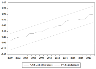
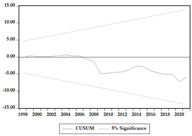
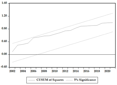
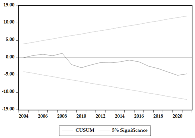
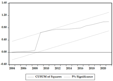
All obtained models were subjected to diagnostic tests of correctness and fit, such as serial correlation (LM test) [45] and heteroskedasticity (ARCH test) tests [46], as well as and Breusch–Pagan–Godfrey evaluations [47]). In addition, stability was examined graphically using the cumulative sum of squares (CUSUM) and cumulative sum of squares (CUSUMQ) measures [48].

4. Empirical Results and Discussion

In this section, the results of the tests are presented. First, the results of the unit root tests are shown. Next, the panel co-integration, FMOLS (fully modified ordinary least squares), DOLS (dynamic ordinary least squares), ARDL (autoregressive distributed lag), and causality tests are examined. These tests allow us to assess long-term relationships, adjust for potential endogeneity, and explore causal relationships between variables of interest. Finally, diagnostics were conducted to ensure the robustness and reliability of our findings.

4.1. Results for Unit Root Test

The first stage of the study, following the methodological guidelines, required the variables to be tested for stationarity. For panel data, the second-generation CIPS panel unit root test, the first-generation Pesaran and Shin IPS tests, and the Levin, Lin, and Chu (LLC) test were applied. The Akaike information criterion (AIC) was used to determine the optimal number of lags. The results shown in Table 3 for the CIPS and IPS tests indicate that the variables are stationary at the first difference, while the results of the LLC test indicate that all variables, except lnREW, are stationary at the I(0) level, and all variables are stationary at the first difference. This means the conditions for applying the ARDL model to the panel data are met.
In contrast, Table 4 shows the unit root tests for each country. The study used the standardized tests provided for the ARDL method in the form of the Dickey–Fuller (ADF) test and the Phillips–Perron (PP) unit root test.
The convergent result of both tests at a significance level of 5% confirms the stationarity of the tested time series. According to the data presented in Table 3, all the studied series are stationary in I(1), confirming the applicability of the co-integration test method, based on the ARDL model.

4.2. Co-Integration Results

Table 5 shows the results of the co-integration test for the panel data. Two types of tests were used in the study: the Pedroni test and the Kao test. The results provide strong evidence of a long-term relationship between the analyzed variables. The p-values for most of the Pedroni test statistics indicate the rejection of the null hypothesis of no long-term relationship between the analyzed variables. Also, the Kao test indicates statistical significance at the 5% level. The combined test result indicates a significant and persistent relationship between the variables over a long period of time.
For individual countries, a co-integration test based on ARDL bound testing was performed (Table 6). If the value of the test statistic is less than the lower bound I(0), we have no basis for inferring long-term co-integration. On the other hand, if the value of the F statistic is higher than the upper bound of I(1), then we can assume that co-integration is present. According to the assumed significance level of 5%, co-integration has been confirmed for all countries studied. Given the above, limited correction models (ECMs) were estimated in accordance with the methodology in order to examine the relationships involved.

4.3. Results of Evaluations of Short- and Long-Term Models

Table 7 presents the long-run estimates for the panel data. Due to the few countries in the panel, the FMOLS and DOLS estimators were used to compare the results. According to the results presented in Table 7, the variables are significant in both the DOLS and FMOLS models. In the FMOLS model, the variables lnCO2 and lnNREW are significant at the 5% level, while the variable lnREW is significant at the 10% level. On the other hand, in the DOLS model, the variables lnCO2 and lnNREW are significant at the 1% level, while the variable lnREW is significant at the 5% level. Therefore, with regard to the results of the cointegration tests in Table 5, it should be noted that all variables for the panel models are statistically significant in the long run.
The values of the coefficients for the DOLS panel data indicate that a 1% increase in CO2 emissions leads to a 1.27% decrease in GDP in the long term. A 1% increase in renewable energy consumption leads to a 0.09% increase in GDP. In contrast, an increase in non-renewable energy production generates an increase in GDP of 0.87%. The data for the FMOLS estimator converge and differ, to a small extent. Comparing the two models, the DOLS model has a better fit in terms of the R2 parameter.
Table 8 shows the estimation results of the ARDL-ECM model for individual V4 countries. In the case of Poland, a 1% increase in CO2 emissions generates a negative effect in the form of a 1.85% decrease in GDP in the long run. An analogous observation was found in Hungary, where a 1% increase in CO2 emissions decrease the GDP by 2.95%, and in Slovakia, where it causes a decrease of 1.16%. For the Czech Republic, no significant long-term relationship was found between CO2 and GDP.
Renewable energy consumption impacted GDP in the long run in Hungary, where a 1% increase in renewable energy consumption affected GDP growth by 0.21%, and in Slovakia, the increase was 0.29%. In Poland and the Czech Republic, the long-run coefficient was insignificant for the LnREW variable.
In Poland, the Czech Republic, and Slovakia, on the other hand, GDP in the long term was influenced by non-renewable energy consumption. In Poland, a 1% increase in non-renewable consumption affected GDP growth by 1.68%, in the Czech Republic, GDP growth was impacted by 3.07%, and in Slovakia, it had a negative effect in the form of a 2.03% decrease in GDP.
The analysis of the short-run data presented in Table 9 shows that in all the models tested, the error correction term (ECTt−1) was negative, statistically significant, and between 0 and −1. This indicates that the coefficients of the models were correctly estimated. At the same time, the speed of adjustment to long-run equilibrium varied across countries. The ECT coefficient of −0.98 for Poland suggests that, on average, for a 1% deviation from the long-run equilibrium, the GDP adjusts by about −0.98% towards the equilibrium level over one period. This means that any short-term deviation from the long-term relationship between GDP, renewable energy, non-renewable energy, and CO2 in Poland is corrected relatively quickly. For Hungary: an ECT coefficient of −0.555 indicates that a deviation of 1% from the long-run equilibrium results in a correction of the GDP by about −0.55% towards the equilibrium level. Like Poland, Hungary also shows a relatively rapid adjustment process towards the long-run relationship. For the Czech Republic and Slovakia, lower values of the ECT parameter of 0.34 and 0.33, respectively, were obtained. This means that for these two countries, a 1% deviation from the long-run equilibrium leads to an adjustment of the GDP by around −0.34% towards the equilibrium level within one period.
The results suggest a relatively rapid stabilizing effect, in which any deviations from equilibrium are corrected in individual countries within 2–3 periods, indicating a long-term relationship between GDP, renewable energy, non-renewable energy, and CO2 in the individual countries.

4.4. Causality Results

Table 10 shows the individual results of the Toda–Yamamoto causality test for the countries studied. In analyzing the results obtained for the Czech Republic, a unidirectional relationship was found between CO2 and GDP and between renewable energy consumption (REW) and GDP. It was also found that non-renewable energy (NREW) has a significant impact on GDP.
The results of the causality test for Poland indicate a significant unidirectional causal relationships between GDP and CO2, as well as between non-renewable energy and CO2. A bidirectional relationship was also found between CO2 emissions and renewable energy production.
The causality test results for Hungary suggest no significant causal links between CO2, GDP, and renewable energy. However, there is evidence of unidirectional causality between GDP and non-renewable energy and between non-renewable energy and CO2.
The causality analysis for Slovakia indicates no significant causal relationships between CO2 and GDP. However, there is a significant bidirectional causality between renewable energy and GDP and a unidirectional causality between non-renewable energy and GDP and renewable energy. In addition, a bidirectional relationship between CO2 emissions and non-renewable energy production has also been demonstrated.

4.5. Diagnostics Results

Table 11 displays the diagnostic tests for the tested ARDL-ECM model. Four techniques, namely variable autocorrelation (Breusch–Godfrey LM test), time series heteroskedasticity (Breusch–Pagan–Godfrey heteroskedasticity test and ARCH), and the functional form problem (Ramsey RESET test), were used to identify possible instability. The empirical results displayed in Table 9 suggest that all the tested ARDL-ECM models effectively passed these tests, indicating the absence of bias.
To verify the robustness and validity of the estimated results, we utilized CUSUM and CUSUMSQ tests to evaluate the dynamic stability of the parameters. The graphical representations of these tests are presented in Appendix A. The model is considered stable, since both the data series fall within the present limits, and the coefficients are deemed significant at the 5% significance level.
The robustness checks were carried out indicate that the models obtained are valid. First, two cointegration tests were carried out, and two panel models FMOLS and DOLS were estimated. All data series in the cointegration tests are in agreement in respect to implication and symbol orientation. Also, the CUSUM and diagnostic tests were confirmed to show that all models are stable.

5. Discussion

At the outset, it should be pointed out that it is not straightforward to compare the results obtained with those presented in previous studies, so this section will point out the general common conclusions for this study and other studies. This is firstly due to the different time and spatial sets of previous studies and the datasets and methods used. Secondly, the V4 countries are very often included in broader research categories. Thirdly, for the V4 countries, in the context of the variables studied, the Toda–Yamamoto causality tests were not conducted early on.
The results obtained by the authors for the Visegrad countries indicate that, on an individual (ARDL-ECM model) and panel (FMOLS and DOLS) basis, there is a long-term negative cointegrating relationship between CO2 emissions and economic growth. The results show that a 1% increase in CO2 emissions leads to a decrease in GDP of around 1.26% for the V4 economies. Therefore, these results differ from those found in similar studies using the FMOLS and DOLS methods. Uçak et al. [49], for highly developed OECD countries, indicated that a 1% increase in GDP leads to a 0.86% increase in CO2. Similarly, using the same methods, Mitić et al. [50] found that a 1% change in GDP leads to about a 0.35% change in CO2 in transition economies. Khan et al. [51] also showed a significant long-term impact of GDP on CO2 emissions in ASEAN countries.
In contrast, the results are consistent with those found in the study by Salazar-Núñez et al. [52], which indicated, based on data for the last 50 years, that the relationship between CO2 emissions and GDP growth is negative. This result fits in with studies that suggest that as GDP per capita increases, CO2 emissions initially increase, but then decrease, according to an inverted U-shaped curve [53]. Also, studies regarding the economies of China, Colombia, Ecuador, and Peru indicate that as CO2 emissions increase, GDP per capita tends to decrease [53,54,55,56].
In relating these observations to the results obtained in the study, it is essential to point out the specific characteristics of the V4 countries. Being in the bloc of communist countries until the end of the 1980s, these countries exhibited energy-intensive economies oriented towards concentrated industrial production, often leading to environmental degradation [56]. After the economic transition, the role of industry began to decline, and services began to dominate the production structure. The growth of freedoms and civic initiatives in Eastern and Central Europe also led to greater public involvement, potentially increasing the enforcement of environmental regulations [57]. In addition, due to the increased importance of services and the change in the socio-economic structure in the economies of these countries, dynamic economic growth occurred, with a decrease in greenhouse gas emissions.
The results thus support Hannesson’s hypothesis that CO2 intensity decreases as countries become more prosperous, implying that structural changes in GDP, such as a shift towards services, may not significantly help decarbonization efforts and reduce CO2 [58]. It means that reducing CO2 emissions while achieving economic growth is possible. Given the above, hypothesis H3 can be confirmed, based on the results obtained.
The study also showed that a 1% increase in non-renewable energy production in the Visegrad countries leads to an increase in GDP of about 0.86%, while an increase in renewable energy production leads to an increase in GDP of about 0.09%. Thus, hypotheses H1 and H2 have been positively verified. However, a difference is apparent in the individual models: in the Czech Republic and Hungary, producing both types of energy positively affects GDP growth, with non-renewable energy exerting a stronger effect. In Poland, on the other hand, renewable energy production has a negative impact on GDP in the long term, and the opposite is true in Slovakia.
Previous research shows that non-renewable energy consumption has a positive impact on GDP growth in the long term [59,60]. It has also been shown that an increase in non-renewable energy consumption leads to an increase in real GDP in the short term [61,62]. In contrast, studies in some countries suggest that non-renewable energy consumption has a negative impact on economic growth, while renewable energy consumption has a positive impact on economic growth [4].
In contrast, Sahlian et al., using a sample of 28 European Union countries, indicated that renewable energy can contribute to GDP growth [63]. Also, results for OECD countries confirm the indicated observation for renewable energy production and water [64]. Similar results were also obtained by Alfonso et al. [65], indicating that electricity consumption from renewable sources positively influences growth in Estonia and Sweden.
It is also worth pointing out that some studies indicate that the impact of renewable energy on GDP may vary, depending on the economic development status of a country. In developed economies, higher renewable electricity consumption is associated with higher GDP growth rates [66], while in emerging and developing economies, the relationship appears to be non-linear [67]. This is also indicated by the results of the causality test, which shows the complex relationship between energy production economics and the environment.
In the Czech Republic, CO2 emissions and non-renewable energy affect GDP. In Poland, the links between GDP, CO2 emissions, and non-renewable energy require a balance between economic growth and environmental protection. In Hungary, non-renewable energy affects GDP growth, while the lack of a direct causal links between CO2, GDP, and renewable energy suggests the need for non-renewable resource management. In Slovakia, renewable energy impacts GDP, while non-renewable energy impacts GDP and CO2. In each country, the challenge is to adapt the energy strategy to its unique conditions to achieve sustainable development in the context of global environmental goals. This is consistent with the findings of the study by Papież et al. [20], which utilized a PVAR model, demonstrating that in nations with comparatively advanced renewable energy industries, the economy is stimulated by renewable electricity consumption and vice versa. Given the above rationale and the results obtained, it should be assumed that hypothesis H4 has been positively verified.
The results obtained thus confirm previous observations, while adding new aspects to the existing state of knowledge. As a general reference, it should be pointed out that despite some commonalities, energy production in the individual V4 countries is based on different sources. Thus, the results suggest that the main factor determining the impact of energy production on the GDP is the energy mix. Slovakia, which has a relatively high share of RES and a low share of coal in production compared to other V4 countries, shows a positive impact of increasing production from renewable sources on GDP. The Czech Republic and Hungary, which have a moderate share of coal in energy production, show a positive impact of both renewable and non-renewable energy production on GDP. Poland, where energy production is mainly based on coal, is in the worst position. This means that an increase in energy production from renewable sources must involve significant investment and costs, which can harm long-term economic growth.

6. Conclusions

This study researched the effect of renewable and non-renewable energy consumption and CO2 emissions on economic growth at the V4 Group’s regional level, along with the relationships between selected variables in the individual countries of the group. In order to clarify the indicated relationships based on the latest available data, the FMOLS/DOLS and ARDL approaches were applied, and causality was tested based on the Toda–Yamamoto test. The results obtained confirmed the four assumed research hypotheses.
The main findings of this study are as follows. Firstly, the FMOLS and DOLS results show that renewable energy has a positive, albeit small, impact on economic growth in the panel of countries studied over the long term. By far, the more significant impact is generated by non-renewable energy. Also importantly, a negative impact on economic growth was shown for CO2. This shows that the V4 countries are still dependent on non-renewable energy, and that CO2 emissions burden their economic growth in the long term.
Secondly, from individual studies within the ARDL model, a difference in the direction and significance of the impact of individual variables is apparent. In the case of Poland, Slovakia, and Hungary, a strongly negative effect of CO2 on economic growth can be seen. Also in Poland, the Czech Republic and Slovakia, non-renewable energy had a significant impact on economic growth in the long term, while in Hungary, renewable energy had a significant impact.
The results obtained and the causality test results indicate causality between GDP and CO2 for the Czech Republic and Poland. It indicates that in these two countries, CO2 emissions play a significant role in economic growth. In terms of energy production, in the Czech Republic and Slovakia, economic growth was influenced by renewable energy. At the same time, there was a significant causality between non-renewable energy and economic growth in all countries. In addition, in the case of Poland, it was possible to confirm the relationship between renewable energy and CO2. The overall results showed that the relationship between economic growth, renewable and non-renewable energy production, and CO2 emissions is influenced by economic structural characteristics and the energy structure.
As a result, the results obtained have important policy implications, as they indicate the positive impact of renewable energy production on economic growth in the countries studied. In view of the above, renewable energy sources should be promoted and developed in the V4 countries, since in all the countries studied, except for Poland, they do not hinder GDP growth, but rather stimulate it. In the case of Poland, where energy production is largely based on coal, a rapid transition to renewable energy sources may affect the coal industry, leading to job losses and economic disruption in coal-dependent regions. It is therefore recommended that the country adopts a strategic and comprehensive approach to the transition, providing economic support to the regions and industries affected.
However, it is expected that the promotion and development of renewable energy will have a positive impact on stimulating economic growth, as well as contributing to reducing greenhouse gas emissions or increasing energy security in all V4 countries. The results obtained are therefore part of the ongoing debate on the energy transition in the European Union countries and the achievement of a zero-carbon economy by 2050. The results obtained provide a clear argument for policy makers that the promotion and development of renewable energy does not have a negative impact on the economy, but generates significant benefits in the form of reduced CO2 emissions, which translates into environmental quality. The results also show that renewable energy has a significant impact on economic growth in the countries studied. In this case, instead of a sudden change, a gradual transition to renewable energy is recommended, which will ensure a stable energy supply. A gradual and well-considered transition will help to minimize the negative impact on GDP.
The findings should be of interest to policy makers responsible for implementing energy policies, as they clearly show that energy transition is a positive step. These policies should aim at stimulating low GHG emitting sectors and reducing high GHG emitting sectors. However, they should be implemented responsibly and gradually.

7. Limitations and Future Research

This study has limitations that are worth considering. Firstly, the results are highly dependent on the quality and availability of data, and inaccuracies in the data may introduce errors in the analyses. Secondly, linearity and fixed effects assumptions in the FMOLS and DOLS models may oversimplify complex energy–environment relationships. Thirdly, the selection of variables could impact the results and potentially overlook other essential factors influencing economic growth. Additionally, the phenomenon investigated may be subject to random fluctuations that were not considered in this study.
To mitigate these limitations, future research may benefit from utilizing more advanced econometric methods. Nonlinear approaches, like the nonlinear autoregressive distributed lag (NARDL) and the generalized method of moments (GMM) may offer a resolution, enabling the analysis of more intricate relationships between variables. As the length of the time series increases, additional factors can be incorporated for analysis, without excessive complication of the model. Overall, a more comprehensive and sophisticated approach is needed to gain a better understanding of the complex relationships between energy use, the environment, and economic progress in the Visegrad countries.

Author Contributions

Conceptualization, data curation, writing—original draft preparation, supervision, J.M. and B.S.; methodology, B.S.; software, validation, formal analysis, J.M. and B.S.; investigation, resources, writing—review and editing, J.M. and B.S.; visualization, B.S. All authors have read and agreed to the published version of the manuscript.

Funding

This research was funded by the project within the framework of the Faculty of Economics, West Pomeranian University of Technology in Szczecin, Poland, under the name, “Green Lab: Research and Innovations”.

Data Availability Statement

Conflicts of Interest

The authors declare no conflict of interest.

Appendix A. CUSUM and CUSUMSQ Result for the Estimated Models

Czech Republic
Energies 16 07163 i001Energies 16 07163 i002
Poland
Energies 16 07163 i003Energies 16 07163 i004
Hungary
Energies 16 07163 i005Energies 16 07163 i006
Slovak Republic
Energies 16 07163 i007Energies 16 07163 i008

References

  1. Bhuiyan, M.A.; Zhang, Q.; Khare, V.; Mikhaylov, A.; Pinter, G.; Huang, X. Renewable Energy Consumption and Economic Growth Nexus—A Systematic Literature Review. Front. Environ. Sci. 2022, 10, 878394. [Google Scholar] [CrossRef]
  2. Menegaki, A.N.; Tsani, S. Chapter 5—Critical Issues to Be Answered in the Energy-Growth Nexus (EGN) Research Field. In The Economics and Econometrics of the Energy-Growth Nexus; Menegaki, A.N., Ed.; Academic Press: Cambridge, MA, USA, 2018; pp. 141–184. ISBN 978-0-12-812746-9. [Google Scholar]
  3. Bhat, J.A. Renewable and non-renewable energy consumption—Impact on economic growth and CO2 emissions in five emerging market economies. Environ. Sci. Pollut. Res. 2018, 25, 35515–35530. [Google Scholar] [CrossRef]
  4. Ito, K. CO2 emissions, renewable and non-renewable energy consumption, and economic growth: Evidence from panel data for developing countries. Int. Econ. 2017, 151, 1–6. [Google Scholar] [CrossRef]
  5. Marques, L.; Fuinhas, J.; Marques, A. On the Dynamics of Energy-Growth Nexus: Evidence from a World Divided into Four Regions. Int. J. Energy Econ. Policy 2017, 7, 208–215. [Google Scholar]
  6. Huang, B.-N.; Hwang, M.; Yang, C. Causal relationship between energy consumption and GDP growth revisited: A dynamic panel data approach. Ecol. Econ. 2008, 67, 41–54. [Google Scholar] [CrossRef]
  7. Alper, A.; Oguz, O. The role of renewable energy consumption in economic growth: Evidence from asymmetric causality. Renew. Sustain. Energy Rev. 2016, 60, 953–959. [Google Scholar] [CrossRef]
  8. Esso, J.L. The Energy Consumption-Growth Nexus in Seven Sub-Saharan African Countries. Econ. Bull. 2010, 30, 1191–1209. [Google Scholar]
  9. Fang, Y. Economic welfare impacts from renewable energy consumption: The China experience. Renew. Sustain. Energy Rev. 2011, 15, 5120–5128. [Google Scholar] [CrossRef]
  10. Inglesi-Lotz, R. The impact of renewable energy consumption to economic growth: A panel data application. Energy Econ. 2016, 53, 58–63. [Google Scholar] [CrossRef]
  11. Sebri, M. Use renewables to be cleaner: Meta-analysis of the renewable energy consumption–economic growth nexus. Renew. Sustain. Energy Rev. 2015, 42, 657–665. [Google Scholar] [CrossRef]
  12. Bhattacharya, M.; Paramati, S.R.; Ozturk, I.; Bhattacharya, S. The effect of renewable energy consumption on economic growth: Evidence from top 38 countries. Appl. Energy 2016, 162, 733–741. [Google Scholar] [CrossRef]
  13. Rajaguru, G.; Khan, S.U. Causality between Energy Consumption and Economic Growth in the Presence of Growth Volatility: Multi-Country Evidence. J. Risk Financ. Manag. 2021, 14, 471. [Google Scholar] [CrossRef]
  14. Myszczyszyn, J.; Suproń, B. Relationship among Economic Growth (GDP), Energy Consumption and Carbon Dioxide Emission: Evidence from V4 Countries. Energies 2021, 14, 7734. [Google Scholar] [CrossRef]
  15. Topcu, E.; Altinoz, B.; Aslan, A. Global evidence from the link between economic growth, natural resources, energy consumption, and gross capital formation. Resour. Policy 2020, 66, 101622. [Google Scholar] [CrossRef]
  16. Streimikiene, D.; Kasperowicz, R. Review of economic growth and energy consumption: A panel cointegration analysis for EU countries. Renew. Sustain. Energy Rev. 2016, 59, 1545–1549. [Google Scholar] [CrossRef]
  17. Menegaki, A.N.; Marques, A.C.; Fuinhas, J.A. Redefining the energy-growth nexus with an index for sustainable economic welfare in Europe. Energy 2017, 141, 1254–1268. [Google Scholar] [CrossRef]
  18. Armeanu, D.Ş.; Vintilă, G.; Gherghina, Ş.C. Does Renewable Energy Drive Sustainable Economic Growth? Multivariate Panel Data Evidence for EU-28 Countries. Energies 2017, 10, 381. [Google Scholar] [CrossRef]
  19. Marinaș, M.-C.; Dinu, M.; Socol, A.-G.; Socol, C. Renewable energy consumption and economic growth. Causality Relationship in Central and Eastern European Countries. PLoS ONE 2018, 13, e0202951. [Google Scholar] [CrossRef]
  20. Papież, M.; Śmiech, S.; Frodyma, K. Effects of renewable energy sector development on electricity consumption—Growth nexus in the European Union. Renew. Sustain. Energy Rev. 2019, 113, 109276. [Google Scholar] [CrossRef]
  21. Ozcan, B.; Ozturk, I. Renewable energy consumption-economic growth nexus in emerging countries: A bootstrap panel causality test. Renew. Sustain. Energy Rev. 2019, 104, 30–37. [Google Scholar] [CrossRef]
  22. Costa-Campi, M.; García-Quevedo, J.; Trujillo-Baute, E. Electricity regulation and economic growth. Energy Policy 2018, 113, 232–238. [Google Scholar] [CrossRef]
  23. Gozgor, G.; Lau, C.K.M.; Lu, Z. Energy consumption and economic growth: New evidence from the OECD countries. Energy 2018, 153, 27–34. [Google Scholar] [CrossRef]
  24. Lazăr, D.; Minea, A.; Purcel, A.-A. Pollution and economic growth: Evidence from Central and Eastern European countries. Energy Econ. 2019, 81, 1121–1131. [Google Scholar] [CrossRef]
  25. Muço, K.; Valentini, E.; Lucarelli, S. The relationships between gdp growth, energy consumption, renewable energy production and CO2 emissions in european transition economies. Int. J. Energy Econ. Policy 2021, 11, 362–373. [Google Scholar] [CrossRef]
  26. Myszczyszyn, J.; Suproń, B. Relationship among Economic Growth, Energy Consumption, CO2 Emission, and Urbanization: An Econometric Perspective Analysis. Energies 2022, 15, 9647. [Google Scholar] [CrossRef]
  27. Litavcová, E.; Chovancová, J. Economic Development, CO2 Emissions and Energy Use Nexus-Evidence from the Danube Region Countries. Energies 2021, 14, 3165. [Google Scholar] [CrossRef]
  28. Cialani, C. CO2 emissions, GDP and trade: A panel cointegration approach. Int. J. Sustain. Dev. World Ecol. 2016, 24, 193–204. [Google Scholar] [CrossRef]
  29. Li, R.; Jiang, H.; Sotnyk, I.; Kubatko, O.; Almashaqbeh, I.Y.A. The CO2 Emissions Drivers of Post-Communist Economies in Eastern Europe and Central Asia. Atmosphere 2020, 11, 1019. [Google Scholar] [CrossRef]
  30. Gardiner, R.; Hajek, P. Interactions among energy consumption, CO2, and economic development in European Union countries. Sustain. Dev. 2019, 28, 723–740. [Google Scholar] [CrossRef]
  31. Im, K.S.; Pesaran, M.; Shin, Y. Testing for unit roots in heterogeneous panels. J. Econ. 2003, 115, 53–74. [Google Scholar] [CrossRef]
  32. Unit Root Tests in Panel Data: Asymptotic and Finite-Sample Properties—ScienceDirect. Available online: https://www.sciencedirect.com/science/article/pii/S0304407601000987 (accessed on 20 August 2023).
  33. Pesaran, M.H. A simple panel unit root test in the presence of cross-section dependence. J. Appl. Econ. 2007, 22, 265–312. [Google Scholar] [CrossRef]
  34. Dickey, D.A.; Fuller, W.A. Distribution of the Estimators for Autoregressive Time Series with a Unit Root. J. Am. Stat. Assoc. 1979, 74, 427–431. [Google Scholar] [CrossRef]
  35. Phillips, P.C.B.; Perron, P. Testing for a unit root in time series regression. Biometrika 1988, 75, 335–346. [Google Scholar] [CrossRef]
  36. McCoskey, S.; Kao, C. A residual-based test of the null of cointegration in panel data. Econ. Rev. 1998, 17, 57–84. [Google Scholar] [CrossRef]
  37. Pedroni, P. Purchasing Power Parity Tests in Cointegrated Panels. Rev. Econ. Stat. 2001, 83, 727–731. [Google Scholar] [CrossRef]
  38. Pesaran, M.H.; Shin, Y.; Smith, R.J. Bounds testing approaches to the analysis of level relationships. J. Appl. Econom. 2001, 16, 289–326. [Google Scholar] [CrossRef]
  39. Pedroni, P. Fully Modified OLS for Heterogeneous Cointegrated Panels. In Nonstationary Panels, Panel Co-Integration, and Dynamic Panels; Baltagi, B.H., Fomby, T.B., Carter Hill, R., Eds.; Advances in Econometrics; Emerald Group Publishing Limited: Bingley, UK, 2001; Volume 15, pp. 93–130. ISBN 978-1-84950-065-4. [Google Scholar]
  40. Dreger, C.; Reimers, H.-E. Health Care Expenditures in OECD Countries: A Panel Unit Root and Co-integration Analysis. Int. J. Appl. Econom. Quant. Stud. 2005, 2, 5–20. [Google Scholar] [CrossRef]
  41. Kao, C.; Chiang, M.-H. On the Estimation and Inference of a Cointegrated Regression in Panel Data. In Nonstationary Panels, Panel Co-Integration, and Dynamic Panels; Baltagi, B.H., Fomby, T.B., Carter Hill, R., Eds.; Advances in Econometrics; Emerald Group Publishing Limited: Bingley, UK, 2001; Volume 15, pp. 179–222. ISBN 978-1-84950-065-4. [Google Scholar]
  42. Pesaran, M.H.; Shin, Y. An Autoregressive Distributed-Lag Modelling Approach to Co-integration Analysis. In Econometrics and Economic Theory in the 20th Century: The Ragnar Frisch Centennial Symposium; Strøm, S., Ed.; Econometric Society Monographs; Cambridge University Press: Cambridge, UK, 1999; pp. 371–413. ISBN 978-0-521-63323-9. [Google Scholar]
  43. Engle, R.F.; Granger, C.W.J. Co-Integration and Error Correction: Representation, Estimation, and Testing. Econometrica 1987, 55, 251–276. [Google Scholar] [CrossRef]
  44. Toda, H.Y.; Yamamoto, T. Statistical inference in vector autoregressions with possibly integrated processes. J. Econom. 1995, 66, 225–250. [Google Scholar] [CrossRef]
  45. Breusch, T.S. Testing for autocorrelation in dynamic linear models. Aust. Econ. Pap. 1978, 17, 334–355. [Google Scholar] [CrossRef]
  46. Engle, R.F. Autoregressive Conditional Heteroscedasticity with Estimates of the Variance of United Kingdom Inflation. Econometrica 1982, 50, 987–1007. [Google Scholar] [CrossRef]
  47. Breusch, T.S.; Pagan, A.R. A Simple Test for Heteroscedasticity and Random Coefficient Variation. Econometrica 1979, 47, 1287. [Google Scholar] [CrossRef]
  48. Brown, R.L.; Durbin, J.; Evans, J.M. Techniques for Testing the Constancy of Regression Relationships over Time. J. R. Stat. Soc. Ser. B 1975, 37, 149–163. [Google Scholar] [CrossRef]
  49. Uçak, H.; Aslan, A.; Yucel, F.; Turgut, A. A Dynamic Analysis of CO2 Emissions and the GDP Relationship: Empirical Evidence from High-income OECD Countries. Energy Sources Part B Econ. Plan. Policy 2014, 10, 38–50. [Google Scholar] [CrossRef]
  50. Mitić, P.; Ivanović, O.M.; Zdravković, A. A Cointegration Analysis of Real GDP and CO2 Emissions in Transitional Countries. Sustainability 2017, 9, 568. [Google Scholar] [CrossRef]
  51. Khan, M.W.A.; Panigrahi, S.K.; Almuniri, K.S.N.; Soomro, M.I.; Mirjat, N.H.; Alqaydi, E.S. Investigating the Dynamic Impact of CO2 Emissions and Economic Growth on Renewable Energy Production: Evidence from FMOLS and DOLS Tests. Processes 2019, 7, 496. [Google Scholar] [CrossRef]
  52. Salazar-Núñez, H.F.; Venegas-Martínez, F.; Tinoco-Zermeño, M.Á. Impact of Energy Consumption and Carbon Dioxide Emissions on Economic Growth: Cointegrated Panel Data in 79 Countries Grouped by Income Level. Int. J. Energy Econ. Policy 2020, 10, 218–226. [Google Scholar] [CrossRef]
  53. Daysi, G.; Karla, M.-M.; Paco, A.-S.; Santiago, O.-M. CO2 Emissions, High-Tech Exports and GDP per Capita. In Proceedings of the 2021 16th Iberian Conference on Information Systems and Technologies (CISTI), Chaves, Portugal, 23–27 June 2021; pp. 1–5. [Google Scholar]
  54. Huang, Z. Analyze the Relationship Between CO2 Emissions and GDP from the Global Perspective. In Proceedings of the 2021 International Conference on Financial Management and Economic Transition (FMET 2021), Virtual, 27–29 August 2023; pp. 442–451. [Google Scholar]
  55. Chavaillaz, Y.; Roy, P.; Partanen, A.-I.; Da Silva, L.; Bresson, É.; Mengis, N.; Chaumont, D.; Matthews, H.D. Exposure to excessive heat and impacts on labour productivity linked to cumulative CO2 emissions. Sci. Rep. 2019, 9, 1–11. [Google Scholar] [CrossRef]
  56. Caporale, G.M.; Claudio-Quiroga, G.; Gil-Alana, L.A. CO2 Emissions and GDP: Evidence from China. SSRN J. 2019. [Google Scholar] [CrossRef]
  57. Kochtcheeva, L.V. Environmental Disaster in the Post-Communist Countries: Is There a Solution? Environ. Pract. 2002, 4, 10–13. [Google Scholar] [CrossRef]
  58. Hannesson, R. CO2 intensity and GDP per capita. Int. J. Energy Sect. Manag. 2019, 14, 372–388. [Google Scholar] [CrossRef]
  59. Ali, Q.; Raza, A.; Narjis, S.; Saeed, S.; Khan, M.T.I. Potential of renewable energy, agriculture, and financial sector for the economic growth: Evidence from politically free, partly free and not free countries. Renew. Energy 2020, 162, 934–947. [Google Scholar] [CrossRef]
  60. Shabbir, S.; Zeshan, M.; Muhammad, S. Renewable and Non-Renewable Energy Consumption, Real GDP and CO2 Emissions Nexus: A Structural VAR Approach in Pakistan; University Library of Munich: Munich, Germany, 2011. [Google Scholar]
  61. Belaïd, F.; Zrelli, M.H. Renewable and Non-Renewable Electricity Consumption, Carbon Emissions and GDP: Evidence from Mediterranean Countries. Energy Policy 2019, 133, 110929. [Google Scholar] [CrossRef]
  62. Al-Mulali, U.; Fereidouni, H.G.; Lee, J.Y. Electricity consumption from renewable and non-renewable sources and economic growth: Evidence from Latin American countries. Renew. Sustain. Energy Rev. 2014, 30, 290–298. [Google Scholar] [CrossRef]
  63. Sahlian, D.N.; Popa, A.F.; Creţu, R.F. Does the Increase in Renewable Energy Influence GDP Growth? An EU-28 Analysis. Energies 2021, 14, 4762. [Google Scholar] [CrossRef]
  64. Ohler, A.; Fetters, I. The causal relationship between renewable electricity generation and GDP growth: A study of energy sources. Energy Econ. 2014, 43, 125–139. [Google Scholar] [CrossRef]
  65. Afonso, T.L.; Marques, A.C.; Fuinhas, J.A.; Saldanha, E.M.M. Interactions between electricity generation sources and economic activity in two Nord Pool systems. Evidence from Estonia and Sweden. Appl. Econ. 2017, 50, 3115–3127. [Google Scholar] [CrossRef]
  66. Halkos, G.E.; Tzeremes, N.G. The effect of electricity consumption from renewable sources on countries’ economic growth levels: Evidence from advanced, emerging and developing economies. Renew. Sustain. Energy Rev. 2014, 39, 166–173. [Google Scholar] [CrossRef]
  67. Liu, Y.; Wei, T.; Park, D. Macroeconomic impacts of energy productivity: A general equilibrium perspective. Energy Effic. 2019, 12, 1857–1872. [Google Scholar] [CrossRef]
Table 1. Overview of the newest studies involving V4 countries.
SourceCountryCausalityModelTime
Huang et al. [6]26 OECD countriesEC → GDPVECM and PVAR1971–2016
Rajaguru and Khan [13]48 countriesEC → GDPARDL-
Myszczyszyn and Suproń [14]Visegrad countriesEC ↔ GDPARDL1992–2015
Topcu et al. [15]124 countriesEC → GDPPVAR1980–2018
Streimikiene and Kasperovich [16]EU countriesEC → GDPFMOLS, DOLS1995–2015
Menegaki et al. [17]EU countriesEC ↔ GDPPARDL2000–2012
Armeanu et al. [18]EU countriesREW → GDPPVAR2003–2014
Marinaș et al. [19]CEE countriesREW ↔ GDPARDL1990–2014
Papież et al. [20]EU countriesREW ↔ GDPPVECM1990–2014
Ozcan and Ozturk [21]Emerging countriesREW ≠ GDPCausality panel1990–2016
Costa-Campi et al. [22]EU countriesEC → GDPOLS panel2007–2013
Gozgor et al. [23]OECDNREW → GDP
REW → GDP
ARDL1990–2013
Papież et al. [20]EU countriesREW ≠ GDP
NREW ≠ GDP
PVAR1995–2015
Lazăr et al. [24]CEE countriesCO2 → GDPFMOLS1996–2015
Muço et al. [25]European transition economiesCO2 ↔ GDP
REW → GDP
PVAR1990–2018
Myszczyszyn and Suproń [26]Visegrad countriesCO2 ↔ GDP
EC → GDP
ARDL1992–2016
Litavcová and Chovancová [27]Danube Region countriesMixedARDL1990–2019
Cialani [28]150 countriesCO2 ↔ GDPECM panel1960–2008
Li et al. [29]Post-communist economiesCO2 → GDPOLS panel1996–2018
Gardiner and Hajek [30]EU countriesCO2 → GDP
EC → GDP
PVECM1990–2015
Note: EC—total energy use/consumption; REW—use/consumption of renewable energy; NREW—use/consumption of non-renewable energy; CO2—carbon dioxide emissions; GDP—economic growth. Source: authors’ own concept.
Table 2. Descriptive statistics.
VariableCountryMeanMedianMaxMinStd. Dev.n
lnGDPCzech Republic9.5899.6799.9169.2340.22331
Hungary9.2599.3309.6488.8990.23331
Poland9.0959.1149.6698.4650.36631
Slovak Republic9.3619.4259.8128.7790.34431
lnCO2Czech Republic2.4012.4322.6142.2320.10631
Hungary1.6151.6781.8681.3640.13831
Poland2.0632.0432.2481.9550.08531
Slovak Republic1.7951.8282.0941.4550.12431
lnREWCzech Republic−3.276−3.434−2.346−4.5090.68131
Hungary−4.758−4.140−2.795−6.3831.31931
Poland−3.982−4.405−2.642−4.8450.79631
Slovak Republic−2.517−2.498−2.185−3.4850.29031
lnNREWCzech Republic−0.456−0.382−0.302−0.7170.14231
Hungary−1.225−1.217−1.071−1.3930.07831
Poland−1.068−1.049−0.897−1.2110.08531
Slovak Republic−0.806−0.803−0.658−0.9580.08131
Source: authors’ study.
Table 3. Panel unit root test results (IPS; CIPS; Levin, Lin, and Chu).
VariableLevelFirst Differences
CIPSLevin, Lin, and Chu IPSCIPSLevin, Lin, and Chu IPSCIPS
lnCO2−2.16−1.93 **−2.16−5.63 *−4.97 *−4.48 *−2.16
lnGDP−1.55−1.93 **0.97−3.60 *−4.97 *−4.48 *−1.55
lnNREW−2.07−1.58 *−0.78−4.94 *−4.51 *−5.25 *−2.07
lnREW−1.240.270.67−3.34 *−5.28 *−5.38 *−1.24
Source: authors’ study. Notes: The significance of the coefficients is indicated by an asterisk in the tables, where ***, **, and * denote 5%, 1%, and 0.1% significance levels, respectively.
Table 4. Unit root test results for individual countries (the augmented Dickey–Fuller test (ADF) and the Phillips–Perron test (PP)).
CountryVariableLevelFirst Differences
ADFPPADFPP
t-Statp-Valuet-Statp-Valuet-Statp-Valuet-Statp-Value
Czech RepubliclnGDP−0.810.801−0.360.904−4.110.004−4.460.001
lnNREW−1.560.491−1.540.501−4.900.001−4.940.000
lnREW−1.250.6390.190.967−5.980.000−4.330.002
lnCO2−1.820.363−2.040.271−4.980.000−4.920.000
HungarylnGDP0.260.972−0.360.904−4.600.001−4.460.001
lnNREW−1.490.5260.720.991−5.050.000−4.010.004
lnREW−1.480.5313.301.000−6.130.000−2.970.050
lnCO20.890.994−1.790.379−3.780.033−5.60.000
PolandlnGDP−2.640.0995.081.000−4.690.001−5.160.000
lnNREW−0.610.8540.720.991−4.920.001−4.010.004
lnREW0.930.9952.431.000−4.250.003−4.310.002
lnCO2−2.020.278−2.000.287−5.240.000−5.130.000
Slovak RepubliclnGDP−1.540.502−0.230.923−4.170.003−4.950.000
lnNREW−2.440.1400.720.991−6.140.000−4.010.004
lnREW−1.860.3462.431.000−5.170.000−4.310.002
lnCO2−3.990.005−2.850.064−5.330.000−7.040.000
Source: authors’ study.
Table 5. Panel co-integration test results.
TestStatisticWeighted Statistic
Within-Dimension
v-Statistic panel1.25 ***1.34 ***
rho-Statistic panel−0.67−0.30
PP-Statistic panel−1.84 **−1.46 ***
ADF-Statistic Panel−2.22 **−2.47 *
Between-Dimension
Group rho-Statistic0.62
Group PP-Statistic−2.20 **
Group ADF-Statistic−2.99 *
Kao-Cointegration test
ADF−2.37 *
Notes: The significance of the coefficients is indicated by an asterisk in the tables, where ***, **, and * denote 5%, 1%, and 0.1% significance levels, respectively. Source: authors’ study.
Table 6. Co-integration test results for individual countries (ARDL bound test).
CountryF-Statistics ValueF-StatisticsI(0)I(1)
Czech Republic7.294 *10% 2.676 3.586
5% 3.272 4.306
1% 4.614 5.966
Hungary5.497 **10% 3.097 4.118
5% 3.715 4.878
1% 5.205 6.640
Poland11.492 *10% 3.770 4.535
5% 4.535 5.415
1% 6.428 7.505
Slovak Republic8.227 *10% 3.097 4.118
5% 3.715 4.878
1% 5.205 6.640
Notes: The significance of the coefficients is indicated by an asterisk in the tables, where ***, **, and * denote 5%, 1%, and 0.1% significance levels, respectively. Source: authors’ study.
Table 7. Panel FMOLS and DOLS model estimation results.
VariablesCo-EfficientStd. Errort-StatisticsProb.
DOLS
lnCO2−1.2750.431−2.9590.004
lnNREW0.8570.3502.4470.017
lnREW0.0880.0531.6700.099
R-squared0.870014
FMOLS
lnCO2−1.1020.340−3.2440.002
lnNREW0.9200.3043.0260.003
lnREW0.1120.0472.3880.019
R-squared0.769619
Source: authors’ study.
Table 8. Long-run results of ARDL—ECM for individual countries.
CountryVariablesCo-EfficientStd. Errort-StatisticsProb.
Czech Republic
CO2−1.0880.806−1.3500.188
NREW3.0670.8763.5000.002
REW0.4080.5510.7400.466
PolandConst.2.0980.7672.7340.011
CO2−1.8570.412−4.5110.000
NREW1.6830.6492.5930.015
REW−0.1290.094−1.3740.181
Const.3.1091.0762.8880.008
HungaryCO2−2.9510.542−5.4470.000
NREW0.5230.5151.0150.319
REW0.2050.0583.5630.001
Const.−3.1470.818−3.8490.001
Slovak RepublicCO2−1.1660.523−2.2290.035
NREW−1.9500.491−3.9710.001
REW0.2970.1491.9950.057
Source: authors’ study.
Table 9. Short-run results of ARDL—ECM for individual countries.
CountryVariablesCo-EfficientStd. Errort-StatisticsProb.
Czech RepublicΔlnGDPt−10.4690.1892.4870.021
ΔlnCO20.2871.9160.1500.882
ΔlnCO2t−1−1.6852.122−0.7940.436
PolandΔlnNREW−0.0542.145−0.0250.980
ΔlnNREWt−11.0781.8850.5720.574
ΔlnREW0.5640.4121.3710.185
ΔlnREWt−1−0.2630.355−0.7420.466
ECTt−1−0.3410.155−2.2020.039
ΔlnGDPt−10.4080.1692.4150.025
ΔlnCO2−0.8240.378−2.1790.042
ΔlnCO2t−10.4360.4440.9810.338
ΔlnNREW−0.0800.821−0.0970.923
ΔlnNREWt−10.2221.0200.2180.830
ΔlnREW0.0180.2290.0800.937
ΔlnREWt−10.1720.2180.7890.439
ECTt−1−0.9820.214−4.8290.000
HungaryΔlnGDPt−1−0.2300.167−1.3720.185
ΔlnCO2−0.4550.500−0.9100.374
ΔlnCO2t−10.5840.5910.9870.335
ΔlnNREW−0.0240.421−0.0580.954
ΔlnNREWt−1−0.3290.420−0.7840.442
ΔlnREW−0.0050.102−0.0450.965
ΔlnREWt−10.1150.0931.2300.233
ECTt−1−0.5550.144−3.8410.001
Slovak RepublicΔlnGDPt−10.5240.1782.9420.008
ΔlnCO2−0.6050.524−1.1550.261
ΔlnCO2t−10.4010.6170.6500.523
ΔlnNREW−0.7350.541−1.3590.189
ΔlnNREWt−10.0700.4920.1430.887
ΔlnREW0.2590.1571.6490.114
ΔlnREWt−1−0.0920.153−0.6030.553
ECTt−1−0.3350.161−2.0810.048
Notes: Δ is the first difference operator; ECTt−1 is the error correction term. Source: authors’ study.
Table 10. Toda-–amamoto causality test for individual countries.
Cause → EffectCzech RepublicPolandHungarySlovakia
χ2Prob.χ2Prob.χ2Prob.χ2Prob.
CO2 → GDP18.820.0001.340.8540.140.9345.290.259
GDP → CO22.680.44319.360.0013.570.1683.200.525
GDP → REW0.730.8671.810.7711.210.5479.060.060
REW → GDP14.830.0026.010.1991.730.42011.980.018
GDP → NREW2.290.5145.820.2136.020.0492.420.659
NREW → GDP17.650.0017.790.0951.300.52220.800.001
CO2 → REW0.420.93510.150.0381.070.5857.590.108
REW → CO27.350.06221.180.0004.350.1144.560.335
CO2 → NREW3.670.2991.250.86911.380.0031.080.898
NREW → CO25.660.1298.160.0861.750.4183.790.436
REW → NREW12.610.0064.300.3678.180.0173.620.459
NREW → REW1.070.7854.660.3244.550.10312.190.016
Source: authors’ study.
Table 11. Diagnostics test for models.
CountrySer. Corr χ2
(Breusch-Godfrey LM Test)
Homoskedasticity χ2
(Breusch-Pagan-Godfrey Test)
Heteroskedasticity χ2 Test
(ARCH)
Stable
(Ramsey RESET Test)
Czech Republic0.9100.3560.151Stable
Poland0.5520.4440.582Stable
Hungary0.5910.3970.341Stable
Slovak Republic0.4130.5440.660Stable
Notes: The significance of the coefficients is indicated by an asterisk in the tables, where ***, **, and * denote 5%, 1%, and 0.1% significance levels, respectively. Source: authors’ study.
Disclaimer/Publisher’s Note: The statements, opinions and data contained in all publications are solely those of the individual author(s) and contributor(s) and not of MDPI and/or the editor(s). MDPI and/or the editor(s) disclaim responsibility for any injury to people or property resulting from any ideas, methods, instructions or products referred to in the content.