Lithium-Ion Battery State of Health Estimation Using Simple Regression Model Based on Incremental Capacity Analysis Features

Abstract

Batteries are the core component of electric vehicles (EVs) and energy storage systems (ESSs), being crucial technologies contributing to carbon neutrality, energy security, power system reliability, economic efficiency, etc. The effective operation of batteries requires precise knowledge of the state of health (SOH) of the battery. A lack of proper knowledge of SOH may lead to the improper use of severely aged batteries, which may result in degraded system performance or even a risk of failure. This makes it important to accurately estimate battery SOH using only operational data, and this is the main topic of this study. In this study, we propose a novel method for online SOH estimation for batteries featuring simple online computation and robustness against measurement anomalies while avoiding the need for full cycle discharging and charging operation data. Our proposed method is based on incremental capacity analysis (ICA) to extract battery aging feature parameters and regression using simple piecewise linear interpolation. Our proposed method is compared with back-propagation neural network (BPNN) regression, a popular method for SOH estimation, in case studies involving actual data from battery aging experiments under realistic discharging and temperature conditions. In terms of accuracy, our method is on par with BPNN results (about 5% maximum relative error), while the simplicity of our method leads to better computation efficiency and robustness against data anomalies.

1. Introduction

The integration of sustainable energy resources is an important means to achieve highly set goals in climate and emission control. Lithium-ion batteries (LIBs) play an important role in this effort due to their advantages, such as high energy density, lightweight, low self-discharging rate, and longevity. LIBs have vast applications in consumer electronics, electric vehicles (EVs), energy storage systems (ESSs), etc. [1]. To ensure safety and reliability in LIB operations, a battery management system (BMS) is needed. However, after repeated use, the state of health (SOH) of an LIB decreases. Decreased SOH will lead to a decreased capacity for energy storage, decreased current and power output, prolonged charging time, and even instability inside the battery. Typically, when the SOH reaches 80%, the battery should be replaced. To properly use the battery, the BMS must maintain an accurate estimate of the SOH at all times. Online SOH estimation of LIBs is the main topic of this study.

Previous methods to estimate LIB SOH have included those mentioned in the studies of [2,3,4,5,6,7,8,9,10,11,12,13,14,15,16,17,18,19,20,21,22,23,24,25,26]. These methods can be categorized into three groups [3]: experimental techniques, adaptive models, and degradation mechanism detection. Experimental techniques seek to measure the SOH directly or indirectly without relying on mathematical models. A particular experimental method is based on internal resistance measurement [4]. It measures the sudden change in voltage during instants of charging or discharging and uses Ohm’s law to estimate the internal DC resistance of the battery. However, since this method considers only internal DC resistance but not the transient characteristics of the battery, the accuracy of SOH estimation is relatively low. To rectify the situation, the method based on impedance measurement utilizes electrochemical impedance spectroscopy (EIS) [5,6] and measures the AC impedance of the battery by injecting input signals at multiple frequencies. This results in a much more accurate SOH estimate. However, the method of EIS requires sophisticated equipment, and it is not suitable for consumer product use during operation (e.g., on an EV).

In the method of adaptive models, a mathematical model is first built to relate the SOH and the measurable quantities (e.g., voltage and current). Then, the model is used to estimate SOH when the measurements are obtained during operations. Plett et al. [7,8] use a Kalman filter to construct the desired model relating SOH to measurements. Prasad et al. [9] use an electrochemical model (EM) with parametric battery impedance, the value of which can be determined with operational data. Luo et al. [10] use artificial neural networks to construct a relationship between battery SOH and measured battery internal impedance based on the EIS method. The authors of [11,12] directly build an artificial neural network regression model based on online voltage measurements.

The method of degradation mechanism detection seeks to establish the relationship between voltage and SOH during the aging process of the battery. Dubarry et al. [13,14,15,16,17] inspected the open circuit voltage between the positive and negative electrodes of aging batteries and concluded that the voltage was mainly affected by the loss of active material (LAM) and the loss of lithium inventory (LLI). Dubarry continued to study the link between voltage and charge, and developed the theory into incremental capacity analysis (ICA) based on the derivative of charge with respect to voltage (i.e., dQ/dV). ICA is effective at describing the aging process of batteries. However, the ICA curve is found to be sensitive to voltage measurement anomalies, and this sensitivity significantly affects the accuracy of SOH estimation. In order to improve the ICA curve, smoothing techniques are applied. Wu et al. [18,19,20] developed an ICA method based on voltage measurements with fixed voltage intervals. However, this method is inconsistent with the measuring pattern of most BMSs taking voltage measurements every second. Li et al. [21,22,23] investigated using moving average (MA) and Gaussian smoothing (GS) to eliminate the effect of measurement noise in the ICA curves. Li et al. [20,24,25] investigated using smooth functions, such as Gaussian functions and Lorentzian functions, to represent the ICA curve. However, for this method to work, the parameters of the representing functions need to be determined using non-trivial optimization computation, such as nonlinear least squares. In addition, user discretion is needed to choose the widths and the number of peaks in the ICA curves. Only after ICA curve smoothing can the feature parameters be extracted to characterize the aging progress of the batteries. For example, Zhang et al. [25] use support vector regression (SVR) to construct the relationship between the feature parameters and SOH. Lin et al. [26] use a back-propagation neural network (BPNN) to build a similar relationship. However, these techniques may lead to computation procedures that are overly complicated for online SOH estimation.

This study proposes an online SOH estimation method based on ICA using current and voltage measurements during the battery charging process. Our contributions are as follows: the proposed method does not need operation information from full charging (e.g., from 20% SOC to 90% SOC), making it convenient for online applications. In addition, we propose a technique to smooth the ICA curve, resulting in zero-phase distortion. This is crucial for maintaining the accuracy of the aging feature parameter of the ICA curve peak position, and to the best of our knowledge, it has not been considered before. Furthermore, contrary to the recent trend, in which experiments have been conducted with increasingly complicated regression functions (e.g., deep neural networks), we demonstrate that simple piecewise linear interpolation regression functions suffice for our SOH estimation purpose. As an added benefit, the simplicity of the regression function results in robustness against measurement or numerical truncation errors.

In conjunction with the proposed zero-phase filtering of the ICA curves, this study compares three different methods for voltage measurement data smoothing: moving average, wavelet filtering, and secant approximation. Our experiment indicates that moving average and secant approximation are robust methods to smooth voltage measurement data. In addition, we compare the proposed piecewise linear interpolating functions and artificial-neural-network-based regression functions and find that the former is more suitable for online SOH estimation due to its accuracy, computation efficiency, and robustness against measurement data imperfection and numerical truncation.

The rest of the paper is organized as follows: Section 2 describes how ICA curves are constructed from the original battery operation measurement data. Techniques to obtain smooth ICA curves are also discussed. Section 3 describes the chosen feature parameters to characterize the aging progress of batteries and how the feature parameters can be extracted from the ICA curves. Section 4 describes the adopted mathematical model relating the feature parameters to battery SOH, how the models can be constructed offline, and how they are used online to estimate battery SOH. Section 5 describes the experiment (physical and numerical) to demonstrate the practical performance of the proposed SOH estimation method and discusses its relative advantages and disadvantages in comparison to other available methods. Section 6 concludes the paper.

2. Acquisition and Smoothing of ICA Curve

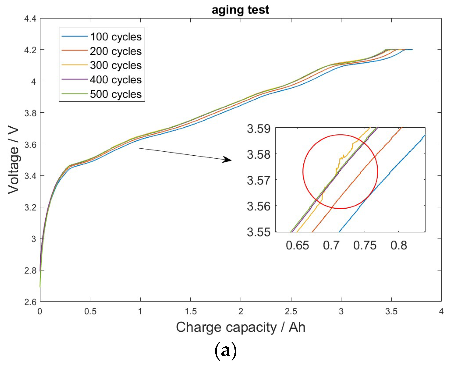
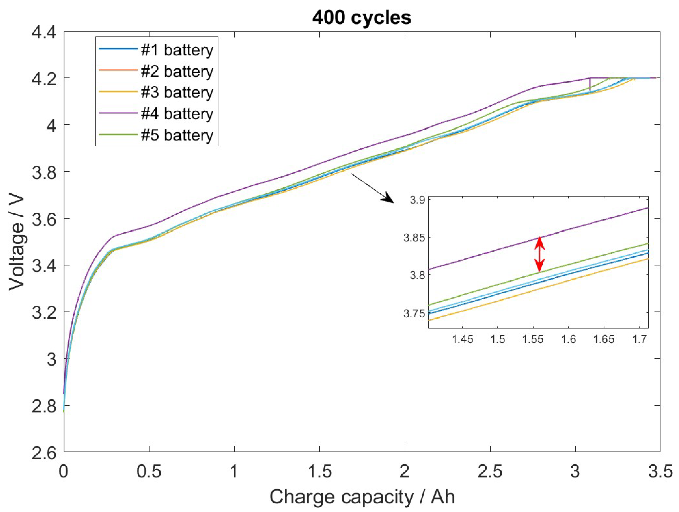
2.1. Construction of the ICA Curve

Typically for constant current (CC) charging, battery operation measurements include current, voltage, and battery charging levels. By using these measurements, the ICA curve can be constructed as follows:

$$ICA=\frac{dQ}{dV}=i\times \frac{dt}{dV}$$

(1)

where Q denotes the charging level (C), V denotes voltage (V), i denotes the constant charging current (A), and t is the variable of time (e.g., seconds). We note that the charging level, Q, is the product of i and t because the current, i, is constant.

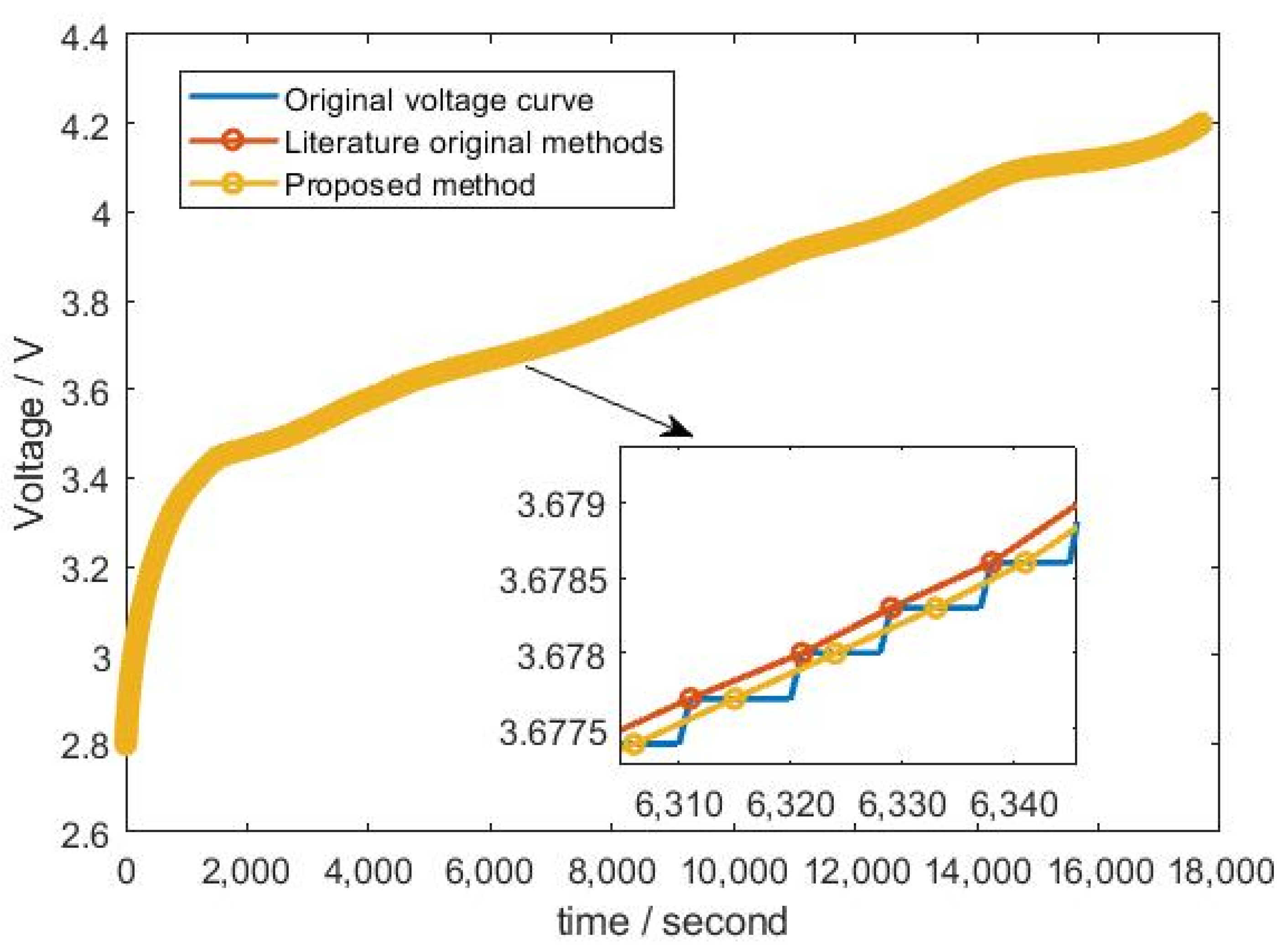
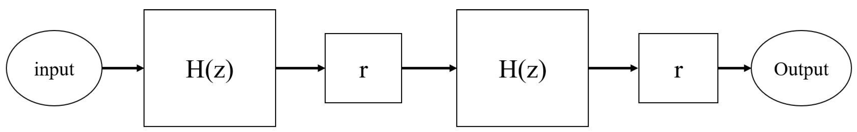
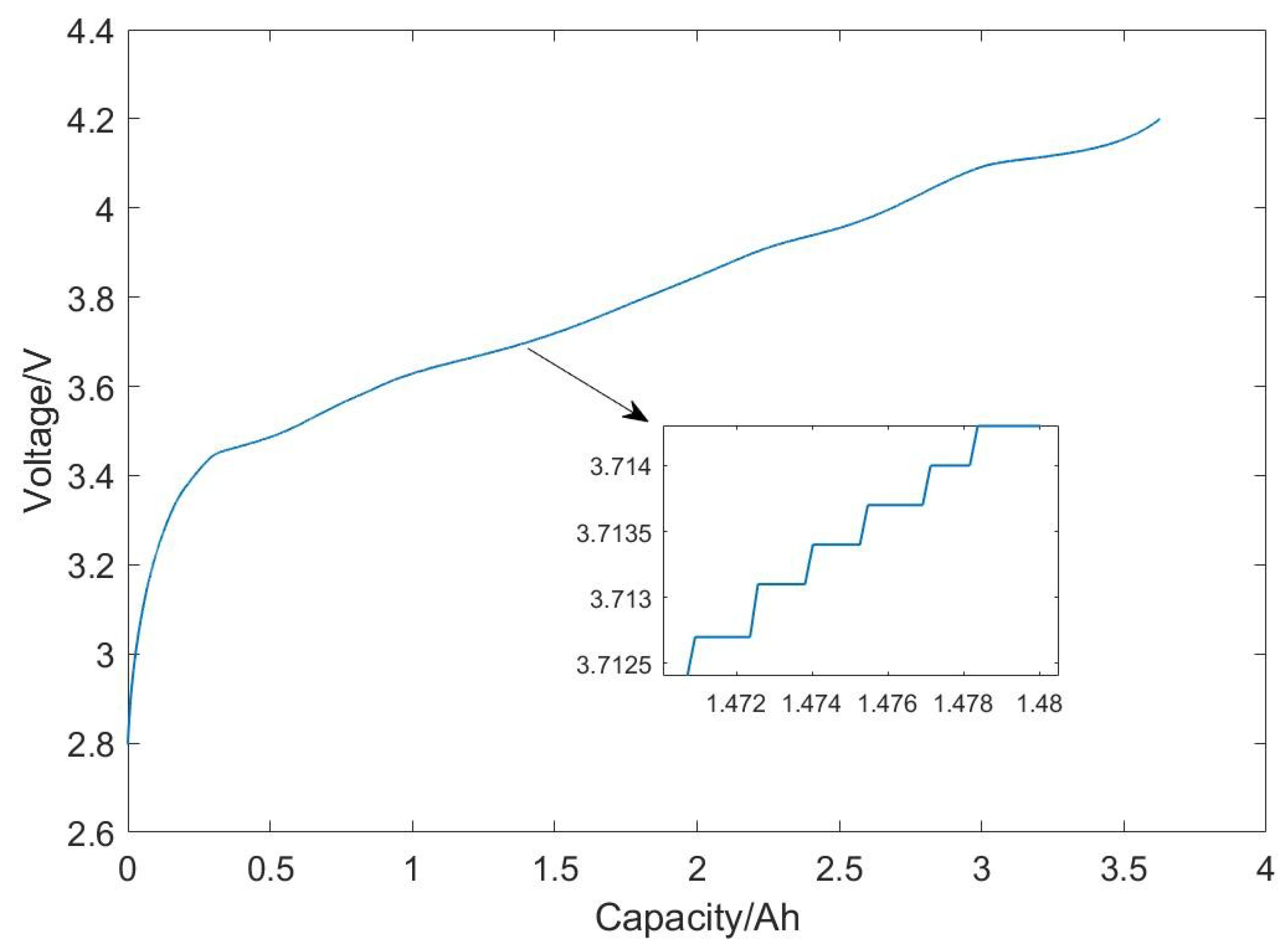
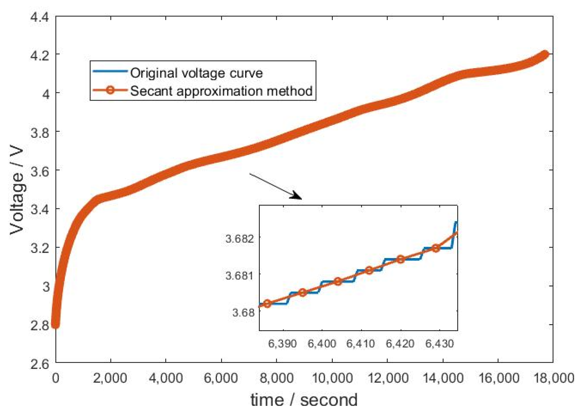
2.2. Voltage Curve Smoothing

By using a typical BMS measurement device, we can obtain a charge (Q)–voltage (V) curve (or Q–V curve for short), as shown in Figure 1. However, quantization error is unavoidable (as shown in the zoomed-in part of Figure 1).

The quantization error of the Q–V curve will lead to significant irregularities in the ICA curve, which will render the subsequent SOH estimation inaccurate. Therefore, smoothing techniques are applied to the Q–V curve to reduce the quantization error. This study compares three different methods for voltage smoothing: moving average, wavelet filtering, and secant approximation.

Moving average (MA) is a standard method to smooth a signal by replacing the signal value at any particular time, t, with the average of signal values taken from a time window starting at some time before t and ending at time t. The size of the time window is a user-specified parameter. In this study, we fix the time window to be 50 time steps (i.e., 50 s). On the other hand, wavelet filtering is also a standard technique to smooth a signal. In this study, the MATLAB command wden.m is employed to transform the original signal into wavelet functions and subsequently quantize the wavelet coefficients based on a threshold, thus accomplishing wavelet filtering.

To remove the quantization effect of the Q–V curve (as shown by the blue line of the zoomed-in part of Figure 2), linear interpolation is applied (as shown by the orange line with circles in the zoomed-in part of Figure 2). This is referred to as the secant approximation method. The “data points” (i.e., orange circles in Figure 2) are chosen to be the mid-points of the plateaus of the Q–V curve, as shown in Figure 2.

To identify the mid-points of the plateaus of the Q–V curve (i.e., the time instants and the corresponding voltage values), we adopt and modify the following procedure from [27], as detailed in Algorithm 1.

Algorithm 1. Secant approximation method algorithm.

1: Initial value i = 1, j = 1, k = 0, p = 2, l = 0

2: V(i) = V(j)  and Record(i) = V(j) and j = j + 1

3: while j ≤ jfinal do

4:  if |V(j) − V(i)| < δ then

5:   k = 0

6:   l = l + 1

7:  else

8:   k = k + 1

9:   if k = 1 then

10:    B1 = V(j)

11:    ID1 = j

12:    B2 = V(j − round(l/2) − 1)

13:    ID2 = j − round(l/2) − 1

14:   else

15:    if k = p then

16:     I = i + 1

17:     V(i) = B1

18:     Record(i) = B2

19:     j = ID1

20:     ix(i) = ID2

21:     l = 0

22:     k = 0

23:    end if

24:   end if

25:  end if

26:  j = j + 1

27: end while

In Algorithm 1, we introduce a variable, l, to keep track of the time duration of the voltage plateaus. Whenever a new value of voltage is encountered (i.e., the “height” of a new plateau), l is reset to zero. The variable, l, increases by one for every time instant until a new voltage value is recorded (i.e., the “height” of the next plateau). At this moment, l is the number of time instants of the current plateau. With this information, the mid-point of the plateau can be inferred. We note that by keeping the mid-points of the plateaus as opposed to the first points of the plateaus, as in [27], the proposed smoothing method achieves an approximation closer to the original quantized Q–V curve, as demonstrated in Figure 3.

In Algorithm 1, the threshold value, δ, is chosen to be 0.001. This is because typical BMS measurements are accurate up to four digits. Furthermore, to conserve BMS memory 152 space and to relieve the online computation burden, the smooth Q–V curve is sub-sampled. For instance, as shown in Figure 3, only the data points corresponding to the yellow circles are stored and processed by the BMS.

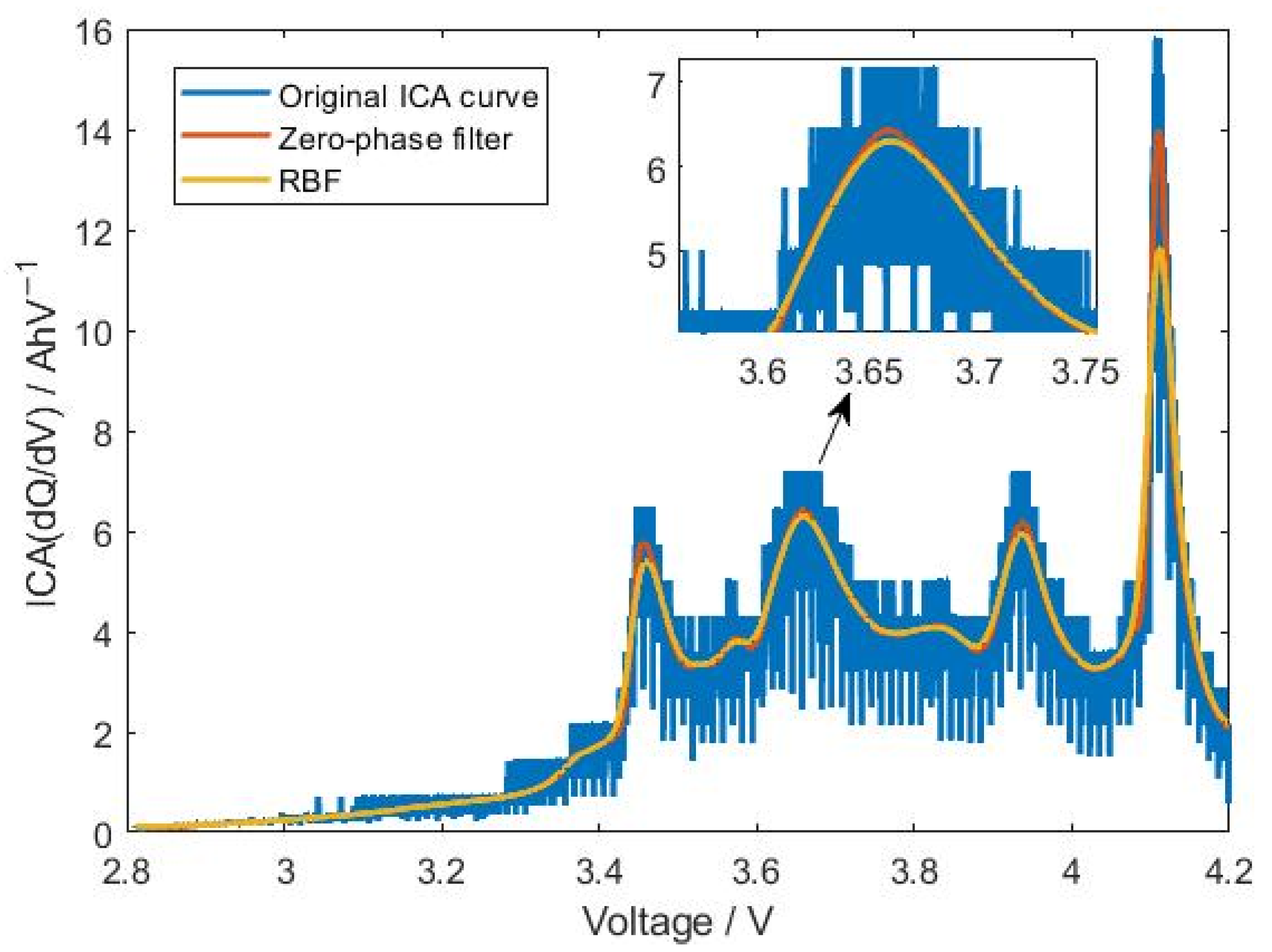
2.3. ICA Curve Smoothing

Even with a smooth Q–V curve, the resulting ICA curve is typically not smooth because of measurement noise, as demonstrated in Figure 4. To accurately extract the aging feature parameters, a smooth version of the ICA curve is usually needed. In this study, we compare two methods for ICA curve smoothing: (a) a smooth basis function regression exemplified by radial basis function (RBF) regression and (b) our proposed method of zero-phase low-pass filtering. RBF regression seeks to approximate the original function (i.e., ICA curve) using linear combinations of basis functions (i.e., Gaussian distribution functions with different means and variances). The weights can be trained offline by minimizing some of the errors between the predicted function output and the actual function output from the data. Low-pass filtering is another typical technique used to construct a smooth ICA curve. However, standard low-pass filtering introduces phase distortion to the filtered ICA curve, which leads to significant inaccuracy in the extracted battery aging feature parameter (e.g., ICA curve peak voltage position). Using linear-phase low-pass filters, such as finite impulse response filters, can alleviate (but not eliminate) the phase distortion issue. However, finite impulse response filters have poor smoothing capability unless the order is unrealistically high (though high orders pose practical implementation issues). In order to both achieve acceptable smoothing performance and avoid phase distortion, this study proposes employing a non-causal zero-phase filtering technique using nonlinear infinite impulse response low-pass filters [28]. A block diagram of non-causal zero-phase filtering is shown in Figure 5.

By first filtering (causally) in the forward direction and then filtering (non-causally) in the reverse direction, phase delays with exactly opposite directions cancel each other so that the output contains zero-phase distortion. The zero-phase filtering shown in Figure 4 can be executed using the MATLAB command filtfilt.m. This study utilizes the Butterworth infinite impulse response filter as H(z) in Figure 4.

Effect of ICA Curve Smoothing

Figure 5 demonstrates the effect of smoothing the ICA curves. It can be seen that even with Q–V curve smoothing, the resulting ICA curve still displays significant irregularities. Battery aging feature parameters can be extracted only after the smoothing of the ICA curves using techniques such as zero-phase filtering or radial basis function regression.

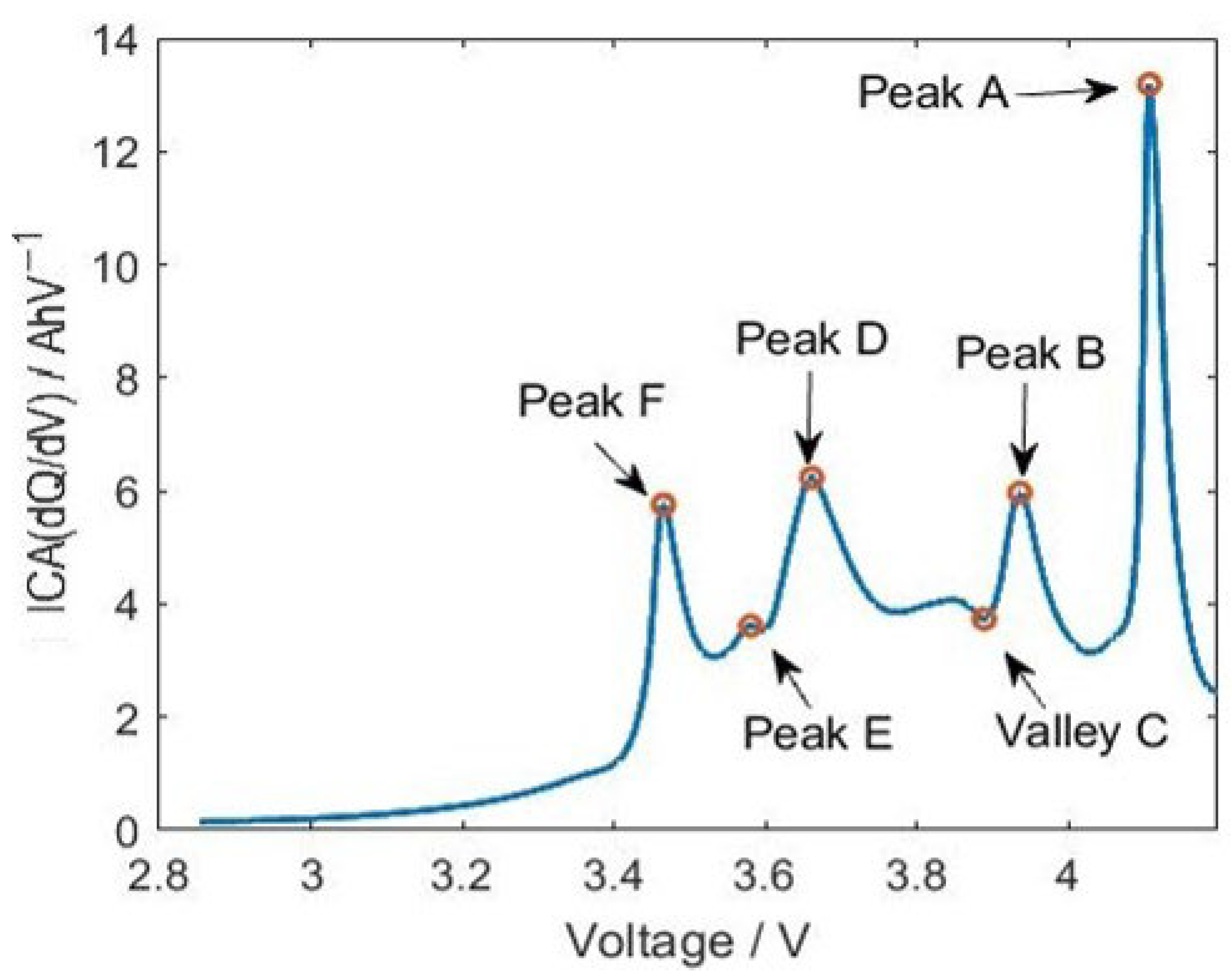
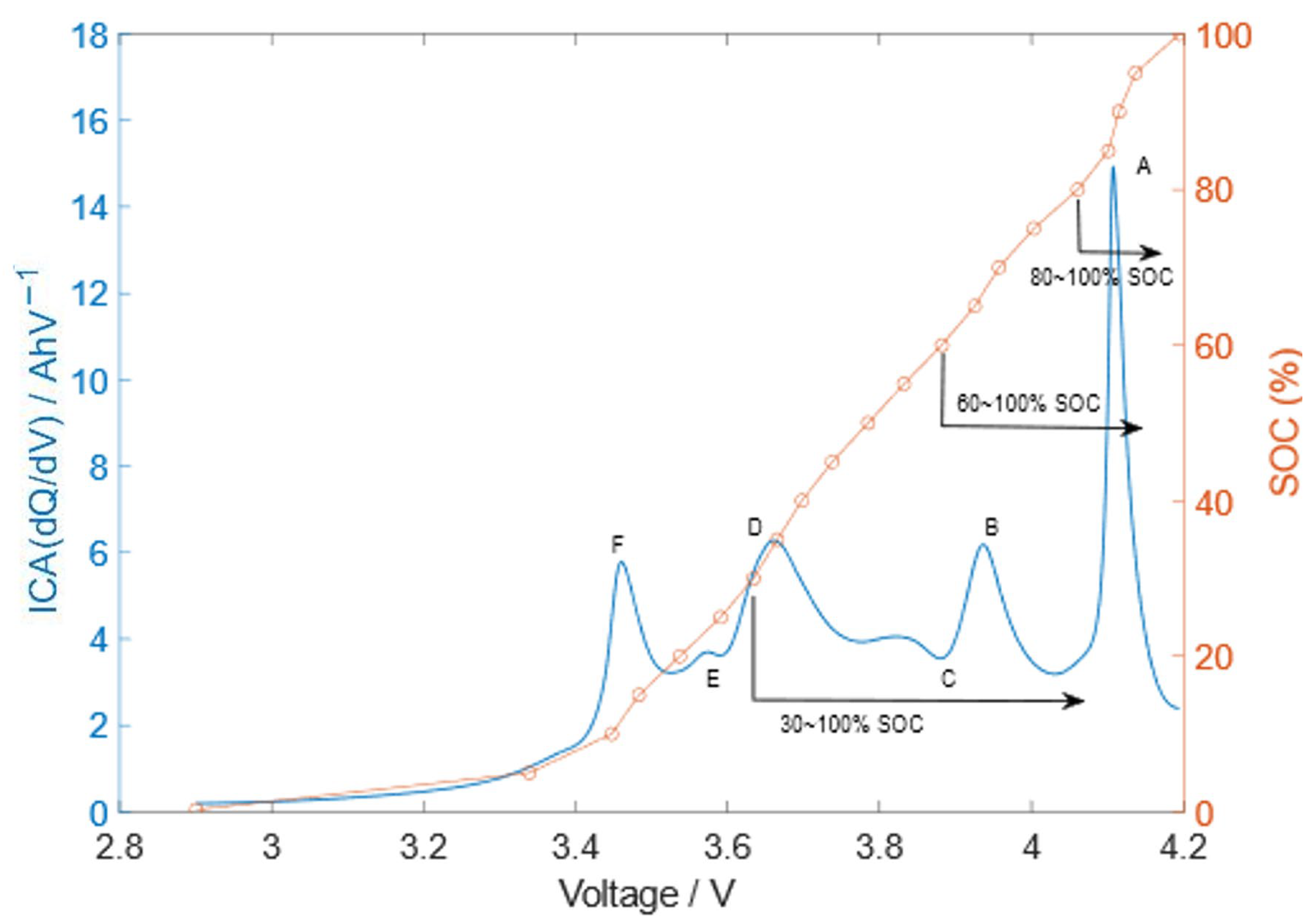
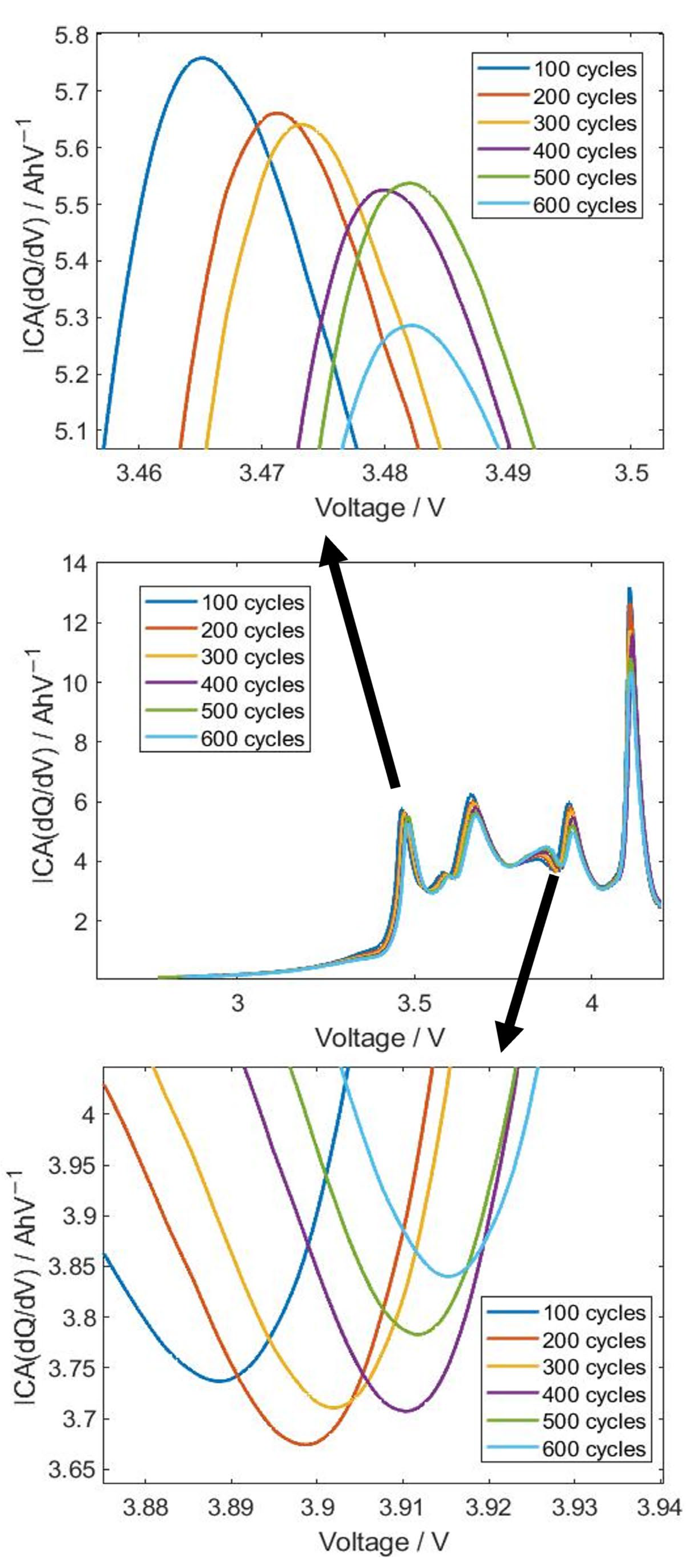
3. Aging Feature Parameter Extraction

After smoothing, the effect of battery aging becomes apparent on the ICA curves. For example, Figure 6 shows six ICA curves for an LIB from 100 to 600 cycles of full discharge and recharge.

Figure 6 shows the trend of the heights of the peaks (and valleys) and the voltage positions of the peaks (and valleys) in the ICA curves. As the number of cycles increases, the heights of the peaks decrease, and the peak voltages increase. For the type of LIBs tested in our studies, we can identify the same number of peaks and valleys in the ICA curves, regardless of the SOH and other operational history. An example ICA curve with some peaks and valleys labeled is shown in Figure 7.

In this study, we identify five peaks and one valley of the ICA curve to define the aging feature parameters for SOH estimation. As indicated in Figure 7, the peaks and valley are peak A, peak B, valley C, peak D, peak E, and peak F. For each peak or valley, the height of the ICA curve and the corresponding voltage value are chosen to be feature parameters to characterize the aging process of the battery. Consequently, in total, there are twelve feature parameters. From our experiment, we can conclude that the peaks and valleys are closely related to the state of charge (SOC) of the battery. Therefore, in operation, the knowledge of current SOC can be used to determine the part of the ICA curve that should be used for SOH estimation. Suppose that, for model building purposes, there are in n total ICA curves corresponding to different SOHs and different operating conditions (temperature, charging current, etc.), the twelve feature parameters for all ICA curves can be assembled into a feature matrix, X, as follows:

$$X={\left[\begin{array}{cccccccc}{P}_{A,h}\left(1\right)& P_{B,h}\left(1\right)& \cdots & P_{F,h}\left(1\right)& P_{A,p}\left(1\right)& P_{B,p}\left(1\right)& \cdots & P_{F,p}\left(1\right)\\ P_{A,h}\left(2\right)& P_{B,h}\left(2\right)& \cdots & P_{F,h}\left(2\right)& P_{A,p}\left(2\right)& P_{B,p}\left(2\right)& \cdots & P_{F,p}\left(2\right)\\ ⋮& ⋮& \ddots & ⋮& ⋮& ⋮& \ddots & ⋮\\ P_{A,h}\left(n\right)& P_{B,h}\left(n\right)& \cdots & P_{F,h}\left(n\right)& P_{A,p}\left(n\right)& P_{B,p}\left(n\right)& \cdots & P_{F,p}\left(n\right)\end{array}\right]}_{\begin{array}{c}n\times 12\end{array}}$$

(2)

where, for instance, P_A,h denotes the height of peak A and P_B,p denotes the voltage position of peak B. To equally emphasize the peaks and valleys, the feature matrix is normalized as follows:

$$X_{norm}\left(:,j\right)=\frac{X(:,j)}{\frac{1}{n}{\sum }_{i=1}^{n}X(i,j)}$$

(3)

where X_norm(:, j) denotes column j of the normalized feature matrix, X(:, j) denotes column j of the original feature matrix, and X(i, j) denotes entry (i, j) of X. To examine the relationship between the chosen feature parameters and battery SOH, the Pearson correlation coefficients are calculated according to the following formula:

$$r\left(x,y\right)=\frac{{\sum }_{i=1}^n(x_i-\overline{X})(y_i-\overline{Y})}{\sqrt{{\sum }_{i=1}^n{\left(x_i-\overline{X}\right)}^2}\sqrt{{\sum }_{i=1}^n{\left(y_i-\overline{Y}\right)}^2}}$$

(4)

where x_i and y_i denote the ith data point of a feature parameter and the corresponding SOH value, respectively. In addition, X and Y represent the average values of vector x and vector y, respectively, over all available data points, corresponding to the rows of the matrix, X_norm. By definition, the Pearson correlation coefficient, r, is between −1 and 1. If r is close to one in absolute value, then x and y are close to linearly related. On the other hand, if r is small in absolute value, then x and y are not related.

Table 1. Pearson correlation coefficients between aging feature parameters and SOH.

Feature Parameter	Peak or Valley Name	Correlation Coefficient
	Peak A	−0.10301
	Peak B	−0.73225
Position	Valley C	−0.84532
	Peak D	−0.75366
	Peak E	−0.52812
	Peak F	−0.64102
	Peak A	0.9636
	Peak B	0.9519
Height	Valley C	0.17517
	Peak D	0.94085
	Peak E	0.88985
	Peak F	0.77354

shows the Pearson correlation coefficients.

From Table 1, we can conclude that SOH is strongly related to the heights of all peaks, except for valley C. On the other hand, SOH is related to the positions of peak B, valley C, and peak D. The values in Table 1 suggest the relevance of the chosen feature parameters.

4. SOH Estimation Methods

To estimate battery SOH based on the feature parameters, it is first necessary to construct regression functions capable of returning the feature parameters for sufficiently representing the values of SOH. Once the regression functions have been constructed, online SOH estimation can be performed based on the principle of residual minimization. For instance, suppose f is a regression function such that y = f (s) is the vector of feature parameters for a given SOH value, s. Then, in operation, when the feature parameter vector is known to be $\widehat{y}$ (from measurements), the SOH estimate can be calculated as $\widehat{s}$ = argmin | f (s) − $\widehat{y}$|.

In this study, two types of regression functions are considered.

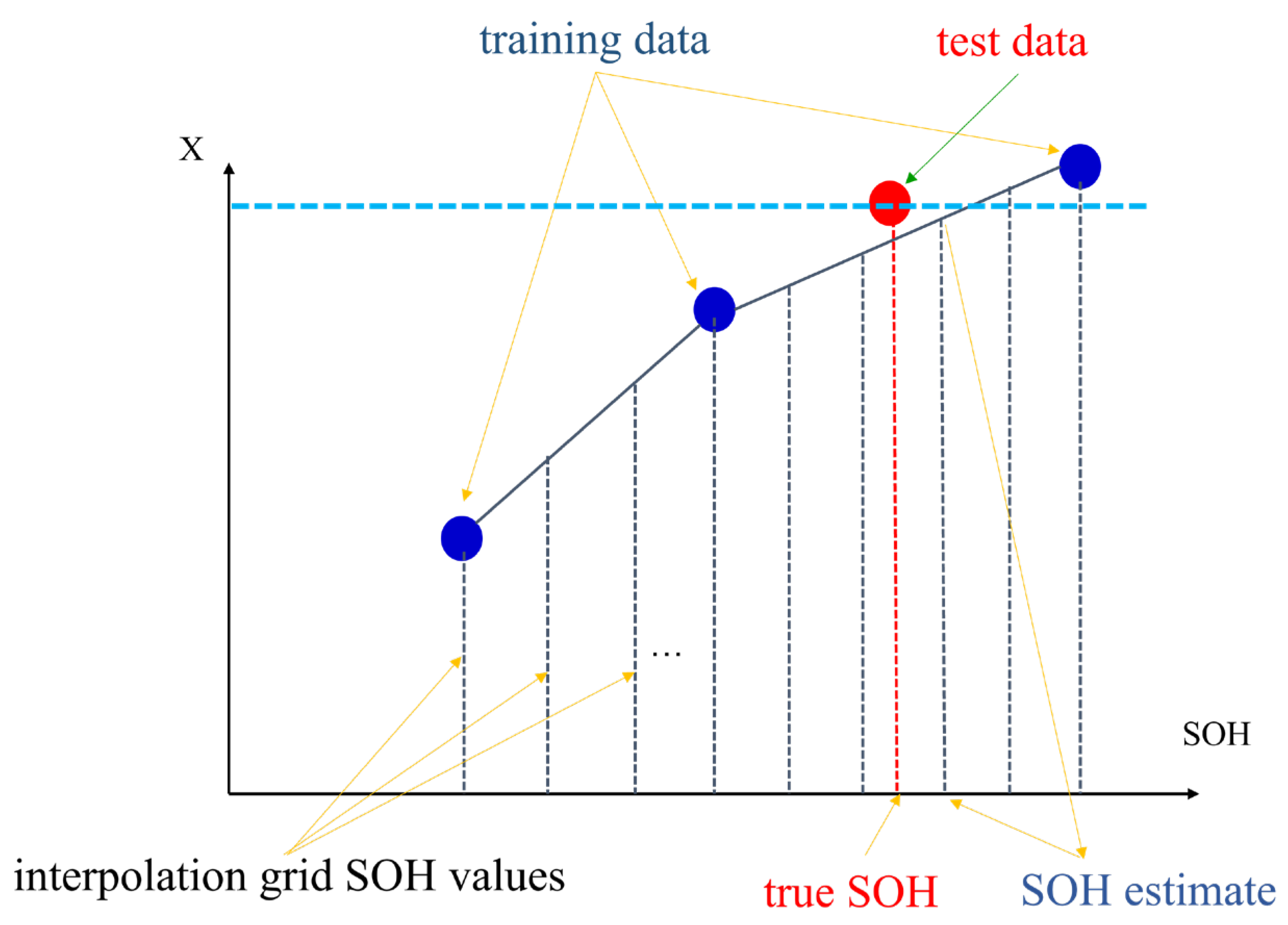
4.1. Piecewise Linear Regression Function

Each row of matrix X_norm in (3) is a normalized feature vector corresponding to a battery SOH value. Thus, the SOH values of all rows form an SOH grid, which may not be uniform. To enable SOH estimation, feature vector values are first interpolated on a uniform SOH grid. Suppose s₁, s₂, and s_n are values of SOH corresponding to the rows of X_norm. Assume that s₁ ≤ s₂ ≤ s_n; then, the uniform SOH grid for interpolation is defined by s₁′, s₂′, …, s′N′ such that s₁ = s₁′ ≤ s₂′ ≤ s′N′ = s_n, s₂′ − s₁′ = s₃′ − s₂′ = …, and N′ is a large number (e.g., 10,000 in this study). Then, given any i [1, N′], the interpolated feature (row) vector is as follows:

$$X^{\prime }\left(i,:\right)=\frac{s_i^{\prime }-s_{n_i}}{s_{n_i+1}-s_{n_i}}\times X_{norm}\left(n_i,:\right)+\frac{s_{n_i+1}-s_i^{\prime }}{s_{n_i+1}-s_{n_i}}\times X_{norm}\left(n_i+1,:\right),\hspace{1em}{s}_{n_i}\le s_i^{\prime }\le s_{n_i+1}$$

(5)

In (5), each si′ corresponds to exactly one s_ni. We assemble all row vectors in (5) into a matrix, X′. Then, X′ can be used to estimate the battery SOH, given the voltage and current measurements in operation. The details are as follows: with voltage and current measurements, a (portion of) smooth ICA curve can be constructed and the (portion of) feature parameters can be identified. Let J ⊆ {1, 2, …, 12} denote the column indices of X′ corresponding to feature parameters that can be identified from the measurements (e.g., the heights and the voltages of peak D and peak E of the ICA curve). Let $\widehat{y}$ be the vector of feature parameters extracted based on the measurements. Then, the SOH estimate is defined using the principle of minimum residual as follows:

$$\widehat{s}=s_{\widehat{\iota }} \mathrm{w}\mathrm{i}\mathrm{t}\mathrm{h} \widehat{\iota }=\underset{i}{\mathrm{argmin}}‖X^{\prime }\left(i,\mathcal{J}\right)-\widehat{y}‖$$

(6)

The principle of SOH estimation in (6) where = 1 (i.e., involving only one feature) is illustrated in Figure 8.

Our proposed piecewise-linear-interpolation-based SOH estimation method requires a grid of discrete SOH values, with N′ being the number of grid points. The choice of N′ represents a trade-off between SOH estimation accuracy and online computation burden.

In principle, the piecewise-linear-interpolation-based method can be applied without first imposing a discrete SOH grid. However, this will significantly complicate online computation because of the identification index, n_i, in (5).

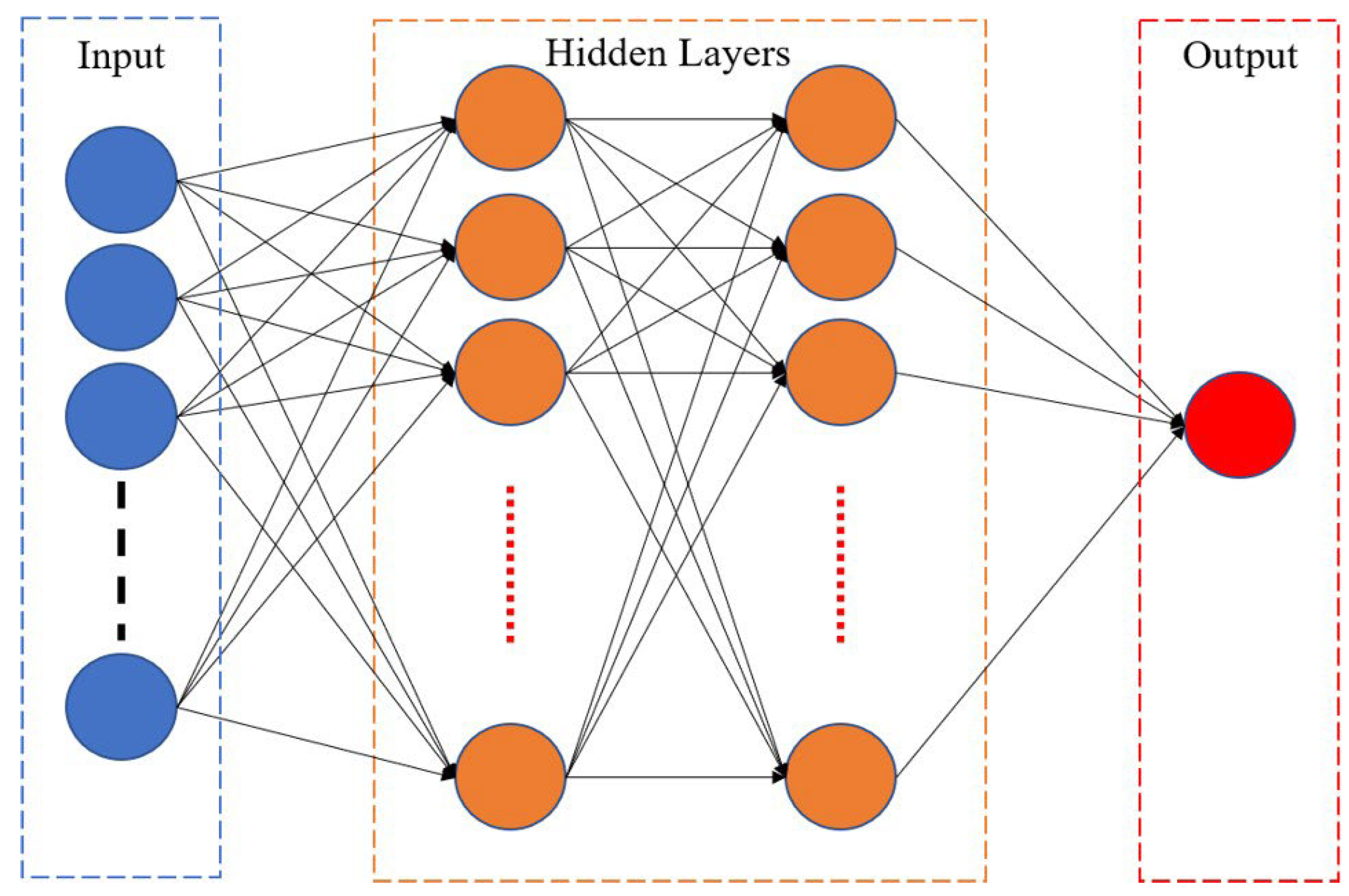
4.2. Back-Propagation Neural Network

To obtain a regression function (for SOH estimation) available for the arbitrary values of SOH, we utilize a back-propagation neural network. The details are as follows: an artificial neural network consists of three types of layers: an input layer, a hidden layer, and an output layer, as shown in Figure 9.

In this study, we use a back-propagation neural network (BPNN) to construct the regression function. The computation process involving BPNN consists of two parts: forward propagation and backward propagation. In forward propagation, starting from the input layer, the weighted sums of the inputs to one layer pass through nonlinear activation functions to form the outputs of the layer (i.e., the input to the next layer). The mathematical expression is as follows:

• Neural input:

  wx + b

  (7)
• Neural output:

  y = f (wx + b)

  (8)

where x is the input vector, w is the weight vector, b is the offset vector, f is the activation function, and y is the output vector. Forward propagation evaluates the values of the outputs (i.e., feature vector) given the inputs to the neural network (i.e., SOH). The function is parameterized by the activation function, f, and the weights, w, and offsets, b. Typically, the activation is pre-specified, while the weights and offsets are optimized during the neural network training process in order to match the desired input–output relationship. The second part of BPNN computation is backward propagation. It evaluates the gradient of the mean squared error between the given and predicted outputs with respect to the weights and the offsets. Using the gradient information, the weights and the offsets can be updated to further reduce the prediction error of the neural network.

We have performed extensive experiments to evaluate BPNNs with different structures and parameters. BPNNs with 2 and 3 hidden layers and 10, 20, and up to 50 neurons per layer are evaluated. In our study, we adopt the specific structure of a BPNN with two hidden layers and 10 neurons per layer, achieving the best trade-off between (offline and online) computation requirements and accuracy. Our BPNN-related results in the numerical study in Section 5 will focus exclusively on the BPNN with our adopted structure and parameter values. The activation function is chosen to be the sigmoid function, and the output layer utilizes linear functions. We use Matlab’s deep neural network toolbox to train the BPNNs with the following algorithmic parameters: Levenberg–Marquardt algorithm for back-propagation, MSE error objective, and an early stop value of 10.

5. Test Results and Discussions

In this section, we evaluate the performance of the proposed SOH estimation method using data from aging experiments with real batteries. We compare variants of the proposed method with different methods for ICA curve smoothing and regression function building (piecewise linear interpolation versus BPNN). Also, the proposed method based on ICA is compared with a neural network regression method using direct voltage measurements, as described in [11,12].

5.1. Physical Experiment Settings

In our experiment, lithium nickel manganese cobalt oxide (NMC) LIBs are used. The proportion of the battery materials is LiNi_0.8 Mn_0.1Co_0.1O₂ (NMC811) [29]. The typical maximum capacity of NMC21700 LIBs is 4000 mAh. The discharging end voltage and charging end voltage are 2.75 V and 4.2 V, respectively. Further details about the tested batteries can be found in [30,31].

The aging experiment is conducted with eight test groups subject to different combinations of operation temperatures and discharge currents. The possible combinations of the testing conditions are summarized in

Table 2. Battery test conditions.

Temperature	Charge Current (C-Rate)	Discharge Current (C-Rate)
25 °C	0.2 C	0.2 C, 0.5 C, 1 C, 2 C
45 °C	0.2 C	0.2 C, 0.5 C, 1 C, 2 C

. We note that our aging experiment is conducted with a standard charge current value of 0.2 C. In actual operation, the charge current may be slightly different from 0.2 C. However, owing to the continuity of physical quantities and the robustness of our proposed method (to be demonstrated later in this section), we expect our method to perform reasonably well, even if the charge current is not exactly at 0.2 C.

Each test group contains eight batteries. The charging mode is constant current and constant voltage (CC-CV) charging from 0% SOC to 100% SOC. When a battery is fully charged, constant current (CC) discharging is applied in stages until the battery is fully discharged. Each stage reduces the battery SOC by 10% and is followed by a resting period of 30 min. Discharging continues until the SOC drops to 0% when the battery is fully charged again. Each test battery undergoes 600 cycles of the aforementioned full charging and discharging. The SOH of the batteries is recorded for every 100 cycles of charging and discharging.

For online SOH estimation application, it is rarely possible to fully discharge and then fully charge the battery. Hence, it is not always possible to perform SOH estimation based on all twelve aging features. Figure 10 shows the portions of the ICA curves that can be constructed based on voltage and current measurements for different ranges of battery SOC. Figure 10 suggests that when SOC is around 80%, the ICA curve is around peak A.

When SOC is between 55% and 65%, the ICA curve is between peak B and valley C.

Considering the fact that charging typically begins when the SOC is relatively low, in our experiment setting, the SOC is assumed to be around 30%, and we evaluate our SOH estimation method based only on the four aging features related to peak D and peak E. We have also evaluated our method for other SOC values including peak E and peak F, peak B and valley C, and peak A and peak B. Experiments with these SOC values lead to similar conclusions to that obtained by our study involving peak D and peak E. Hence, we focus our subsequent discussions assuming the SOC is about 30%.

5.2. SOH Estimation Computational Experiment Settings

The normalized ICA-based feature vector adopted in our experiment is as follows:

X₁ = Norm(P_D,h, P_E,h, P_D,p, P_E,p)

(9)

where P_D,h, P_E,h, P_D,p, and P_E,p denote the heights and voltage positions of peak D and peak E, respectively. The features are extracted from a charging process beginning 1 min before peak E and lasting for 30 min. Inspired by [11,12], we also experiment with the choice of normalized feature vector based directly on voltage measurements (without using the ICA curve) as follows:

X₂ = Norm(V₀, V_i, V_DTi, V_PTi)

(10)

In (10), V₀ denotes the initial voltage measurement, i is the time index such that instance V₁ denotes the voltage 10 min after the beginning of the charging process. V_DTi denotes the difference, V_iV₀, and V_PTi denotes the relative version of V_DTi. Equation (3) is used for the normalization in (9) and (10).

The SOH estimation procedures evaluated in our experiment can be categorized into four groups: (a) ICA with piecewise linear interpolation regression (a variant of the proposed method), (b) ICA with BPNN regression (a variant of the proposed method), (c) piecewise linear interpolation regression using voltage measurements (from [11,12]), and (d) BPNN regression using voltage measurements (from [11,12]). For (a) and (b), we further evaluate sub-variants due to different methods for voltage curve smoothing (i.e., zero-phase filtering and radial basis function regression) and ICA curve smoothing (i.e., moving average, wavelet filtering, and secant approximation). Details of the four experiment groups are as follows:

(a)

ICA with piecewise linear interpolation regression:

For each instance of the experiment, 70% of the data is randomly chosen as “training data” to find feature vectors of the form X₁ in (9). These feature vectors then form matrix X′ according to (5). Once matrix X′ is constructed, it is used for SOH estimation according to (6), and the estimation procedure is evaluated using the remaining 30% of (validation) data. Multiple instances of the aforementioned random experiment are conducted (with the random selection of 70% of training data) to compute the statistics (i.e., average) of the SOH estimation performance metrics. After extensive trials, we fix the number of random instances at 10,000 in order to calculate sufficiently accurate averages.

(b)

ICA with BPNN regression:

Similar to (a), for each instance of the experiment, 70% of the data is randomly chosen to be “training data” to find feature vectors of the form X₁ in (9). These feature vectors are used to train the artificial neural network with the early stopping option. The neural network is used for SOH estimation, and its performance is evaluated using the remaining 30% of the data. A total of 10,000 instances of random experiments are conducted to compute the statistics of the performance of the BPNN-based SOH estimation method.

(c)

Piecewise linear interpolation regression using voltage measurements:

Similar to (a), for each instance of the experiment, 70% of the data is randomly chosen to be “training data”. The training data are used directly to form feature vectors of the form X₂ in (10). These feature vectors then form matrix X′ according to (5). Once matrix X′ is constructed, it is used for SOH estimation according to (6), and the estimation procedure is evaluated using the remaining 30% of (validation) data. A total of 10,000 instances of random experiments are conducted to compute the statistics of the performance of the SOH estimation method, based on piecewise linear interpolation regression and direct voltage measurements.

(d)

BPNN regression using voltage measurements:

Similar to (b), for each instance of the experiment, 70% of the data is randomly chosen to be “training data”. The training data are used directly to form feature vectors of the form X₂ in (10) to train the artificial neural network with the early stopping option. The neural network is used for SOH estimation and its performance is evaluated using the remaining 30% of the data. A total of 10,000 instances of random experiments are conducted to compute the statistics of the performance of the BPNN-based SOH estimation method.

5.3. Error Metrics

For each instance of the random experiment, let (si∗, sˆ_i), where i = 1, 2, and M denotes the pairs of true SOH value and SOH estimate corresponding to the validation data (i.e., the 30% of data not used for training). We examine three performance metrics: mean relative error (MRE), root mean squared relative error (RMSRE), and maximum relative error (MAX). The errors are defined as follows:

$$\mathrm{M}\mathrm{R}\mathrm{E}=\frac{1}{M}\sum _{i=1}^M\left|\frac{s_i^{*}-\widehat{s_i}}{s_i^{*}}\right|$$

(11)

$$\mathrm{R}\mathrm{M}\mathrm{S}\mathrm{R}\mathrm{E}=\frac{1}{M}{\sum _{i=1}^M\left(\frac{s_i^{*}-\widehat{s_i}}{s_i^{*}}\right)}^2$$

(12)

$$\mathrm{M}\mathrm{A}\mathrm{X}=\underset{i=1,\dots ,M}{\max }\left|\frac{s_i^{*}-\widehat{s_i}}{s_i^{*}}\right|$$

(13)

5.4. Results: Comparing Combinations of Smoothing and Regression Techniques

Table 3. Comparison of different voltage smoothing methods using zero-phase filters and piecewise linear interpolation of SOH estimation.

Voltage Smoothing Method	MRE (%)	RMSRE (%)	MAX (%)
MA	0.6327	0.917	4.978
Wavelet filtering	0.6548	0.9338	4.975
Secant approximation	0.6028	0.8848	4.862

shows the percentage errors of ICA-based SOH estimation with piecewise linear interpolation regression and zero-phase filtering of the voltage curve, averaged over 10,000 random experiment instances.

Table 4. Comparison of different voltage smoothing methods using RBF and piecewise linear interpolation of SOH estimation.

Voltage Smoothing Method	MRE (%)	RMSRE (%)	MAX (%)
MA	0.6331	0.923	4.988
Wavelet filtering	0.6483	0.9334	4.9881
Secant approximation	06211	0.9198	5.264

shows similar statistics to those in Table 3, except that voltage smoothing is performed using a radial basis function regression instead of zero-phase filtering. From Table 3 and Table 4, we can see, regardless of voltage and ICA curve smoothing techniques, that the errors due to ICA-base SOH estimation with piecewise linear interpolation regression are generally modest. The MAX error due to secant approximation and radial basis function regression is slightly larger but the MRE and RMSRE errors are slightly smaller.

Table 5. Comparison of different voltage smoothing methods using zero-phase filters and BPNN of SOH estimation.

Voltage Smoothing Method	MRE (%)	RMSRE (%)	MAX (%)
MA	0.547	0.729	12.096
Wavelet filtering	0.5773	0.7721	17.897
Secant approximation	0.5246	0.704	11.88

and

Table 6. Comparison of different voltage smoothing methods using RBF and BPNN of SOH estimation.

Voltage Smoothing Method	MRE (%)	RMSRE (%)	MAX (%)
MA	0.5481	0.773	14.598
Wavelet filtering	0.5753	0.7753	16.189
Secant approximation	0.5479	0.7405	16.307

show the error statistics analogous to Table 3 and Table 4, respectively, except that BPNN regression is used instead of piecewise linear interpolation while constructing regression function for SOH estimation. It can be seen that the MRE and RMSRE errors due to BPNN regression are generally smaller than those due to piecewise linear interpolation. On the other hand, the MAX errors due to BPNN tend to be significantly larger. The difference is particularly obvious for the wavelet filtering case.

5.5. Results: Comparing Choices of Aging Feature Parameters

From Table 3, Table 4, Table 5 and Table 6, we can conclude that the combination of zero-phase filtering and secant approximation for ICA curve smoothing delivers the best performance regardless of whether piecewise linear interpolation or BPNN is used for the regression function for SOH estimation. Therefore, for subsequent analysis, we focus on this combination for ICA curve smoothing. Next, we further investigate the effect of the feature vector (ICA-based X₁ in (9) versus voltage-based X₂ in (10)) on SOH estimation performance. The errors are shown in

Table 7. Compare estimates for different input parameters.

Estimation Method	Input	MRE (%)	RMSRE (%)	MAX (%)
Piecewise linear interpolation	X1	0.6028	0.8848	4.862
Piecewise linear interpolation	X2	1.2742	1.697	8.5536
BPNN	X1	0.5246	0.704	11.88
BPNN	X2	1.0255	1.291	10.523

. It can be concluded that the proposed use of the ICA-based feature vector, X₁, generally leads to better accuracy than using the voltage-based feature vector, X₂.

5.6. Discussions on Robustness against Data Anomalies and Truncation Error

In Table 5 (using BPNN as a regression function for SOH estimation), the MAX error for wavelet filtering is about 17%. This is significantly larger than the approximately 12% errors due to other ICA curve smoothing techniques (moving average and secant approximation). A further study into the data reveals a voltage measurement error of a battery during the charging stage of the 300th cycle in the aging experiment. This is illustrated in Figure 11 (the yellow lines in the voltage curve and in the ICA curve).

After removing the abnormal measurement, the MAX error due to wavelet filtering reduces to about 12% while the MAX errors due to moving average and secant approximation remain approximately the same. This indicates that wavelet filtering is more sensitive to errors in measurement data. On the other hand, with or without removing the measurement error, the SOH estimation errors using piecewise linear interpolation regression (cf. Table 3 and Table 4) remain at approximately 5%. This indicates that the proposed piecewise-linear-interpolation-based method is robust against measurement errors.

To further investigate robustness against measurement anomalies, Figure 12 shows the charging stage of the five batteries during the 400th cycle of the aging experiment. It can be seen that the voltage of battery 4 is higher than that of the other batteries. This results in an early switch from constant-current charging to constant-voltage charging for battery 4, and a corresponding shift in the ICA curve voltage position for the battery (to a higher voltage).

Table 8. Effect of measurement errors on SOH estimation.

	Estimation Method	MRE (%)	RMSRE (%)	MAX (%)
Measurement error included	Piecewise linear interpolation	0.6028	0.8848	4.862
	BPNN	0.5246	0.704	11.88
Measurement error not included	Piecewise linear interpolation	0.6025	0.8856	4.862
	BPNN	0.523	0.7086	8.462

shows the errors in the variants of the proposed SOH estimation method with and without removing the measurement outlier shown in Figure 12. The results in Table 8 are obtained using secant approximation and zero-phase filtering for ICA curve smoothing. Table 8 indicates again that MAX error is the most sensitive, and piecewise linear interpolation is generally more robust than BPNN for constructing the regression function for SOH estimation.

To emulate the effect of finite precision online computation using embedded equipment, the case study is repeated using 4-digit calculations instead of 16-digit calculations (default in MATLAB). In this case study, the combination of zero-phase filtering and secant approximation is used in conjunction with piecewise linear interpolation or BPNN regression function for the final SOH estimation.

Table 9. SOH estimation errors due to different choices of computation precision.

Estimation Precision	MRE (%)	RMSRE (%)	MAX (%)
Piecewise linear high precision	0.6028	0.8848	4.862
interpolation low precision	0.6022	0.8834	4.864
BPNN high precision	0.5246	0.704	11.88
low precision	0.5282	0.7094	10.925

indicates that the overall effect of computation precision is insignificant for the proposed SOH estimation procedure.

6. Conclusions

This study has demonstrated that ICA is a promising way to define aging features for LIB SOH estimation. However, to properly use ICA, smoothing is needed before and after the construction of the ICA curves. The study results suggest that battery aging features induced by ICA curves are generally insensitive to the choice of ICA curve smoothing considered in this study, even though our proposed zero-phase filtering and secant approximation techniques tend to deliver the best overall performance in SOH estimation with very modest estimation error (about 5% maximum relative error). While an artificial neural network is a popular choice for SOH estimation regression in conjunction with ICA, our work in this study demonstrates that a simpler procedure based on piecewise linear interpolation suffices, with an additional benefit of robustness against measurement outliers and numerical truncation errors. This is particularly relevant for embedded online applications where measurement anomalies are expected and computation resources are limited. Nevertheless, this study is based on experiments using only lithium-ion batteries. For other types of batteries (e.g., lead–acid batteries), the corresponding ICA curves may be different; hence, a general investigation and guarantee for all battery types is desired. Furthermore, while this study focuses on SOH estimation, the assumption of known SOC is not always valid (e.g., lead–acid batteries). In practice, it is sometimes necessary to jointly estimate SOC and SOH together. The extension of the ICA framework to joint estimation could bring the method even closer to real-world applications.

References

1. Silvestri, L.; De Santis, M.; Mendecka, B.; Bella, G. Identification of the Best Vehicle Segment for e-Taxis from a Life Cycle Assessment Perspective (No. 2022-24-0020); SAE Technical Paper; SAE: Byron Bay, Australia, 2022. [Google Scholar]
2. Han, X.; Lu, L.; Zheng, Y.; Feng, X.; Li, Z.; Li, J.; Ouyang, M. A review on the key issues of the lithium ion battery degradation among the whole life cycle. ETransportation 2019, 1, 100005. [Google Scholar] [CrossRef]
3. Berecibar, M.; Gandiaga, I.; Villarreal, I.; Omar, N.; Van Mierlo, J.; Van den Bossche, P. Critical review of state of health estimation methods of Li-ion batteries for real applications. Renew. Sustain. Energy Rev. 2016, 56, 572–587. [Google Scholar] [CrossRef]
4. Wei, X.; Zhu, B.; Xu, W. Internal resistance identification in vehicle power lithium-ion battery and application in lifetime evaluation. In Proceedings of the 2009 International Conference on Measuring Technology and Mechatronics Automation, Zhangjiajie, Hunan, 11–12 April 2009; Volume 3, pp. 388–392. [Google Scholar]
5. Andre, D.; Meiler, M.; Steiner, K.; Walz, H.; Soczka-Guth, T.; Sauer, D.U. Characterization of high-power lithium-ion batteries by electrochemical impedance spectroscopy. II: Modelling. J. Power Sources 2011, 196, 5349–5356. [Google Scholar] [CrossRef]
6. Chayambuka, K.; Cardinaels, R.; Gering, K.L.; Raijmakers, L.; Mulder, G.; Danilov, D.L.; Notten, P.H. An experimental and modeling study of sodium-ion battery electrolytes. J. Power Sources 2021, 516, 230658. [Google Scholar] [CrossRef]
7. Plett, G.L. Extended Kalman filtering for battery management systems of LiPB-based HEV battery packs: Part 1. Background. J. Power Sources 2004, 134, 252–261. [Google Scholar] [CrossRef]
8. Remmlinger, J.; Buchholz, M.; Meiler, M.; Bernreuter, P.; Dietmayer, K. State-of-health monitoring of lithium-ion batteries in electric vehicles by on-board internal resistance estimation. J. Power Sources 2011, 196, 5357–5363. [Google Scholar] [CrossRef]
9. Prasad, G.K.; Rahn, C.D. Model based identification of aging parameters in lithium ion batteries. J. Power Sources 2013, 232, 79–85. [Google Scholar] [CrossRef]
10. Luo, Y.F.; Lu, K.Y. An online state of health estimation technique for lithium-ion battery using artificial neural network and linear interpolation. J. Energy Storage 2022, 52, 105062. [Google Scholar] [CrossRef]
11. Chen, R.J.; Hsu, C.W.; Lu, T.F.; Teng, J.H. Rapid SOH estimation for retired lead-acid batteries. In Proceedings of the 2021 IEEE International Future Energy Electronics Conference (IFEEC), Taipei, Taiwan, 16–19 November 2021; pp. 1–4. [Google Scholar]
12. Teng, J.H.; Chen, R.J.; Lee, P.T.; Hsu, C.W. Accurate and Efficient SOH Estimation for Retired Batteries. Energies 2023, 16, 1240. [Google Scholar] [CrossRef]
13. Dubarry, M.; Liaw, B.Y.; Chen, M.S.; Chyan, S.S.; Han, K.C.; Sie, W.T.; Wu, S.H. Identifying battery aging mechanisms in largeformat Li ion cells. J. Power Sources 2011, 196, 3420–3425. [Google Scholar] [CrossRef]
14. Dubarry, M.; Truchot, C.; Liaw, B.Y. Synthesize battery degradation modes via a diagnostic and prognostic model. J. Power Sources 2012, 219, 204–216. [Google Scholar] [CrossRef]
15. Birkl, C.R.; Roberts, M.R.; McTurk, E.; Bruce, P.G.; Howey, D.A. Degradation diagnostics for lithium ion cells. J. Power Sources 2017, 341, 373–386. [Google Scholar] [CrossRef]
16. Dubarry, M.; Anseán, D. Best practices for incremental capacity analysis. Front. Energy Res. 2022, 10, 1023555. [Google Scholar] [CrossRef]
17. Fly, A.; Chen, R. Rate dependency of incremental capacity analysis (dQ/dV) as a diagnostic tool for lithium-ion batteries. J. Energy Storage 2020, 29, 101329. [Google Scholar] [CrossRef]
18. Wu, J.; Su, H.; Meng, J.; Lin, M. State of Health Estimation for Lithium-Ion Battery via Recursive Feature Elimination on PartialCharging Curves. IEEE J. Emerg. Sel. Top. Power Electron. 2022, 11, 131–142. [Google Scholar] [CrossRef]
19. Li, X.; Wang, Z.; Zhang, L.; Zou, C.; Dorrell, D.D. State-of-health estimation for Li-ion batteries by combing the incrementalcapacity analysis method with grey relational analysis. J. Power Sources 2019, 410, 106–114. [Google Scholar] [CrossRef]
20. Li, X.; Jiang, J.; Chen, D.; Zhang, Y.; Zhang, C. A capacity model based on charging process for state of health estimation of lithium ion batteries. Appl. Energy 2016, 177, 537–543. [Google Scholar] [CrossRef]
21. Li, Y.; Abdel-Monem, M.; Gopalakrishnan, R.; Berecibar, M.; Nanini-Maury, E.; Omar, N.; van den Bossche, P.; Van Mierlo, J. A quick on-line state of health estimation method for Li-ion battery with incremental capacity curves processed by Gaussian filter. J. Power Sources 2018, 373, 40–53. [Google Scholar] [CrossRef]
22. Li, X.; Yuan, C.; Li, X.; Wang, Z. State of health estimation for Li-Ion battery using incremental capacity analysis and Gaussian process regression. Energy 2020, 190, 116467. [Google Scholar] [CrossRef]
23. Schaltz, E.; Stroe, D.I.; Nørregaard, K.; Ingvardsen, L.S.; Christensen, A. Incremental capacity analysis applied on electric vehiclesfor battery state-of-health estimation. IEEE Trans. Ind. Appl. 2021, 57, 1810–1817. [Google Scholar] [CrossRef]
24. Tang, X.; Liu, K.; Lu, J.; Liu, B.; Wang, X.; Gao, F. Battery incremental capacity curve extraction by a two-dimensional Luenberger–Gaussian-moving-average filter. Appl. Energy 2020, 280, 115895. [Google Scholar] [CrossRef]
25. Zhang, Y.; Liu, Y.; Wang, J.; Zhang, T. State-of-health estimation for lithium-ion batteries by combining model-based incrementalcapacity analysis with support vector regression. Energy 2022, 239, 121986. [Google Scholar] [CrossRef]
26. Lin, H.; Kang, L.; Xie, D.; Linghu, J.; Li, J. Online State-of-Health Estimation of Lithium-Ion Battery Based on Incremental Capacity Curve and BP Neural Network. Batteries 2022, 8, 29. [Google Scholar] [CrossRef]
27. Zheng, Y.; Ouyang, M.; Li, X.; Lu, L.; Li, J.; Zhou, L.; Zhang, Z. Recording frequency optimization for massive battery data storage in battery management systems. Appl. Energy 2016, 183, 380–389. [Google Scholar] [CrossRef]
28. Wanhammar, L.; Saramäki, T. Frequency-Selective Filters. In Digital Filters Using MATLAB; Springer International Publishing: Cham, Switzerland, 2020; pp. 40–55. [Google Scholar]
29. Becker, M.; Zhao, W.; Pagani, F.; Schreiner, C.; Figi, R.; Dachraoui, W.; Grissa, R.; Kühnel, R.-S.; Battaglia, C. Understanding the Stability of NMC811 in Lithium-Ion Batteries with Water-in-Salt Electrolytes. ACS Appl. Energy Mater. 2022, 5, 11133–11141. [Google Scholar] [CrossRef]
30. Molicel Co., Ltd. Lithium-ion Rechargeable Battery Product Data Sheet. 2019. Available online: https://www.molicel.com/wp-content/uploads/INR21700P42A-V4-80092.pdf (accessed on 30 January 2022).
31. IndiaMART. INR-21700-P42A 3.6v Molicel Lithium-ion Battery. Available online: https://www.indiamart.com/proddetail/molicel-lithium-ion-battery-22854981788.html (accessed on 30 January 2022).
Figure 1. A typical Q–V curve during the charging operation of a lithium-ion battery. The zoomed-in part shows the quantization error in the voltage measurement.
Energies 16 07066 g001
Figure 2. Secant approximation method.
Energies 16 07066 g002
Figure 3. A comparison between the proposed secant approximation (yellow line) and a similar method in [27] (orange line).
Energies 16 07066 g003
Figure 4. Zero-phase filtering, where r represents the time-reversal operator of a sequence.
Energies 16 07066 g004
Figure 5. ICA curve before smoothing (blue) and after smoothing using zero-phase filtering (red) or radial basis function regression (yellow).
Energies 16 07066 g005
Figure 6. ICA curves of an LIB after different numbers of cycles of full discharge and recharge.
Energies 16 07066 g006
Figure 7. ICA curve and the chosen peaks and valley.
Energies 16 07066 g007
Figure 8. Illustration of piecewise-linear-interpolation-based SOH estimation involving a single feature. The blue dots (training data) indicate the SOH-feature pairs from offline data. The interpolation grid consists of SOH values s1′, s2′, and sN′, where extra feature values are generated via interpolation if necessary (cf. (5)). The vertical coordinate of the red dot is the value of the measurement-derived feature (i.e., y ^ ), while the horizontal coordinate is the true SOH of the battery. The method of minimum residual in (6) identifies the SOH estimate from the interpolation grid s1′, s2′, and sN′, the feature value of which is closest to the vertical coordinate of the red dot, illustrated as “SOH estimate” in the figure.
Energies 16 07066 g008
Figure 9. The structure of a neural network.
Energies 16 07066 g009
Figure 10. ICA curve for different SOC ranges.
Energies 16 07066 g010
Figure 11. Battery data including measurement errors. (a) Voltage curve. (b) ICA curve.
Energies 16 07066 g011aEnergies 16 07066 g011b
Figure 12. Measurement error of different battery numbers at 400 cycles.
Energies 16 07066 g012