Multi-Objective Dispatch of PV Plants in Monopolar DC Grids Using a Weighted-Based Iterative Convex Solution Methodology

Abstract

The design of an efficient energy management system (EMS) for monopolar DC networks with high penetration of photovoltaic generation plants is addressed in this research through a convex optimization point of view. The EMS is formulated as a multi-objective optimization problem that involves economic, technical, and environmental objective functions subject to typical constraints regarding power balance equilibrium, thermal conductor capabilities, generation source capacities, and voltage regulation constraints, among others, using a nonlinear programming (NLP) model. The main characteristic of this NLP formulation of the EMS for PV plants is that it is a nonconvex optimization problem owing to the product of variables in the power balance constraint. To ensure an effective solution to this NLP problem, a linear approximation of the power balance constraints using the McCormick equivalent for the product of two variables is proposed. In addition, to eliminate the error introduced by the linearization method, an iterative solution methodology (ISM) is proposed. To solve the multi-objective optimization problem, the weighted optimization method is implemented for each pair of objective functions in conflict, with the main advantage that in this extreme the Pareto front has the optimal global solution for the single-objective function optimization approach. Numerical results in the monopolar version of the IEEE 33-bus grid demonstrated that the proposed ISM reaches the optimal global solution for each one of the objective functions under analysis. It demonstrated that the convex optimization theory is more effective in the EMS design when compared with multiple combinatorial optimization methods.

1. Introduction

Monopolar DC grids are emerging technologies that work with direct-current signals to supply electrical energy to multiple users at medium and low-voltage levels [1]. These grids are composed of two poles: one of them is the positive pole that has a voltage of $+V_{DC}$ V concerning the neutral pole that is solidly grounded at each point of load connected, i.e., the neutral pole is set t $0$ V [2]. In these networks, it is possible to connect constant resistive loads (linear loads), constant power loads (nonlinear loads), and distributed energy resources (generation and batteries) [3]. Monopolar DC networks have attracted the attention of researchers and distribution companies since these, when contrasted with AC networks, have better voltage profile performance and low energy losses [4]. The control design is straightforward because the voltage magnitude is the only variable of interest [5].

Two main approaches are reported in the current literature to analyze monopolar DC networks. The first approach is associated with designing control strategies to manage energy flow interchange between the grid and the distributed energy resources connected to it [6]. This is a research area focused on the efficient control of power electronic converters [7], where the primary idea is to support voltage profiles in controlled load terminals, extract the maximum power available in renewable sources, or store energy in batteries during periods of low demand and high generation, to return this energy in periods with contrary behavior [8]. The second approach corresponds to design optimization strategies for planning and operation purposes [9]. In the planning case, the main idea is integrating new devices (renewables or batteries) to improve the grid performance regarding operational costs for an expected horizon period of analysis [10]. In the operation case, usually, the idea is to propose efficient energy management systems that allow defining the best daily power injection profiles for renewable generation and energy storage systems [11,12].

The design of energy management systems (EMSs) is a vast area of research with multiple applications in the contexts of microgrids, and active distribution networks, including applications in seaports [13,14], public buildings [15,16], hospitals [17], farms [18], and electrical distribution networks [11], among others. For this reason, in this research, we are interested in analyzing monopolar DC networks from the optimization point of view by proposing efficient energy management systems (EMS) for monopolar DC grids considering photovoltaic generation [19,20]. Using a multi-objective optimization approach, the proposed EMS considers three objective functions (economic, technical, and environmental) [11]. In the current literature, the EMS for monopolar DC networks has been attracting attention in the last few years. Some of the most relevant reports in this area are presented below.

The authors of [11] have proposed designing an efficient energy management system (EMS) for PV generators integrated into monopolar DC distribution networks considering technical, environmental, and economic objective functions. As constraints, the power balance constraints and the capacities of the devices were considered. A single-objective function analysis was implemented to deal with the exact nonlinear programming (NLP) model. The salp swarm optimization algorithm was implemented to optimize the daily dispatch of the PV generators. Numerical results in two test feeders demonstrated the effectiveness of this optimization algorithm compared to the crow search algorithm, the particle swarm optimizer, and the multi-verse optimization approaches. Ref. [10] proposed a convex approximation based on the McCormick envelopes to select and locate battery energy storage systems in monopolar DC networks. The objective function corresponded to the minimization of the total daily energy losses. Numerical results in the 21-bus grid demonstrated the proposed quadratic convex approximation’s effectiveness when compared with the mixed-integer NLP model’s exact solution in GAMS software. However, the main flaw of this research corresponded to the non-elimination of the error introduced by the McCormick approximation since any recursive optimization approach was implemented. The authors of [12] have proposed a convex optimization method to define the optimal operation of PV sources in monopolar DC networks to minimize the total greenhouse gas emissions in isolated grids fed by diesel generation sources; the main contribution is using artificial neural networks to predict the expected behavior of the power output of the PV sources; numerical results demonstrated that their convex proposal and the exact NLP solution in the GAMS software were the same. Ref. [21] analyzed regulatory scope for integrating renewables in medium and low voltage distribution networks based on the Law 1715 of the Colombian senate. This is the most crucial regulatory scope for integrating any renewable energy resource in the Colombian electric system since this defines all the legal and technical considerations for the massive integration of these devices in the existing passive distribution network, which will cause these networks to become active agents with an essential role in the electricity market. Refs. [22,23] have presented a complete qualitative analysis regarding the integration of PV plants in the Colombian power system. The authors study the market conditions based on the Law 1714 of 2014, considering the active participation of these systems in the new energetic matrix. Qualitative results demonstrate that the Colombian market continues under development areas where more political and economic conditions must be defined before the massive integration of PV generation plants. The authors of [24] proposed the application of a convex approximation based on the branch power flow to determine the efficient dispatch of PV plants in isolated monopolar distribution networks to minimize the total CO${}_2$ emissions caused by diesel sources. Numerical results demonstrated that the branch power flow approach is efficient when the energy losses are minimized; however, when the objective function is different, some convergence problems have been experimented with.

Based on the previous state-of-the-art review, this research contributes the following: (i) a new formulation for the problem of efficient operation of PV plants in monopolar DC networks considering different objective functions. A mathematical analysis is made over each one of these functions to determine their geometric structure, which permits us to confirm that all of them (economic, technical, and environmental) are convex; (ii) the approximation of the nonconvex set of constraints associated with the power balance constraint using the McCormick approximation for the product of two variables. To minimize/eliminate the error introduced by this linearization method, an iterative solution methodology is implemented by starting with plane voltages (equal values in all the nodes) until reaching the desired convergence; (iii) the construction of the Pareto front for each pair of objective functions using the multi-objective weighted-based approach was proposed. Numerical results confirmed that for linear objective function regarding economic or environmental indices, the EMS design is not a multi-objective problem. In contrast, economic/environmental vs. technical are objective functions in conflict.

Note that to demonstrate the effectiveness of the proposed optimization methodology based on convex approximations, a single-objective function analysis with multiple metaheuristics was performed, evidencing that for all the simulation cases, the iterative solution methodology founds better numerical results than the recently reported values with different combinatorial optimization methods reported by Grisales-Noreña et al. in [11]. These comparative algorithms are the crow search algorithm, the particle swarm optimizer, the multi-verse optimizer, and the salp swarm optimization method. On the other hand, it is important to highlight that in this research, the location of the PV plants was previously defined by the distribution company, and the demand and generation curves are considered well-known without uncertainties (input parameters for the studied problem); however, more research will be required to address the stochastic nature of these variables (demand and PV generation curves), added with the possibility of studying the optimal selection of the nodes where the PV plants must be located from the distribution system planning point of view. In addition, the degradation characteristics of the batteries are not considered in this research; however, in future works, it will be necessary to include the aging-degradation characteristics of the batteries, especially for distribution system planning projects that involve energy storage systems.

The remainder of this contribution is organized as follows: Section 2 describes the general EMS using a multi-objective formulation, which considers the minimization of three objective functions: (i) the expected energy losses (technical function); (ii) the expected emissions of CO${}_2$ (environmental function); (iii) the expected energy purchasing costs in conventional generators and maintenance costs of the PV plants (economic function). These objective functions are subject to technical constraints regarding power balance equilibrium, thermal capacities of conductors, generation capacities in power sources, and voltage regulation bounds, among others. Section 3 reveals the proposed solution methodology by presenting the model convexification approaches, followed by the proposed iterative solution methodology. In addition, the multi-objective approach is formally presented using the weighed-based optimization methodology using two factors for combining pairs of objective functions. Section 4 shows the main characteristics of the test feeder under analysis, which corresponds to the monopolar DC version of the IEEE 33-bus grid, including three PV plants with demand and generation behaviors associated with the typical performance of the electrical distribution networks in the Medellín City, Colombia. Section 5 reveals the main numerical results considering a single-objective optimization analysis to compare the performance of the proposed iterative solution methodology with multiple combinatorial optimization methods reported in the specialized literature. In addition, the multi-objective analysis is made to construct the fronts using the weighted-based approach. Finally, Section 6 lists all the conclusions derived from this research and some possible future research works.

2. Multi-Objective Optimization Model

The problem of the efficient operation of PV plants in monopolar DC distribution networks considering different objective functions can be represented as a nonlinear programming model with nonconvex constraints. The main idea of this optimization problem is to find a Pareto front by considering the conflict of interest between different objective functions. Three objective functions are considered in this research, as described below.

2.1. Possible Objective Functions

In modern electrical networks, the economic and environmental indices are fundamental variables that must be considered for reliable and efficient operation at all voltage levels. Here, we evaluate three objective functions regarding technical, economic, and environmental indicators.

The first objective function is typically employed in electrical distribution networks for optimal power flow studies, and it minimizes the expected energy loss for a defined operation horizon ($E_{\mathrm{loss}}$). Equation (1) defines the mathematical structure of this objective function.

$$\begin{array}{c}\hfill min{E}_{\mathrm{loss}}=\sum _{h\in \mathcal{H}}\sum _{km\in \mathcal{L}}{r}_{km}{i}_{km,h}^2{\Delta }_h,\end{array}$$

(1)

where $r_{km}$ is the resistive parameter associated with the distribution line that connects nodes k and m, and $i_{km,h}$ is the current flow at the route $km$ at the period h.

The second objective function is associated with the total greenhouse gas emissions in conventional generation sources (electrical substations in interconnected distribution grids) or diesel generation sources in distribution networks at remote rural distribution grids. This objective function is formulated in Equation (2).

$$\begin{array}{c}\hfill min{E}_{{\mathrm{CO}}_2}=\sum _{h\in \mathcal{H}}\sum _{k\in \mathcal{N}}\left({\gamma }_{cg}{p}_{k,h}^{cg}+{\gamma }_s{p}_{k,h}^s\right){\Delta }_h,\end{array}$$

(2)

where $E_{{\mathrm{CO}}_2}$ is the total greenhouse gas emissions associated with coat dioxide (CO${}_2$), which is the main pollutant in electrical networks based on thermal sources; ${\gamma }_{cg}$ and ${\gamma }_s$ mean the emission coefficients associated with the thermal sources (diesel plants) and the substation equivalents (slack sources), which have power outputs per period defined as $p_{k,h}^{cg}$ and $p_{k,h}^s$, respectively.

The third objective function corresponds to the economic indicator of the grid operation, which is associated with the expected energy generation costs in the case of diesel sources or energy purchasing costs from the transmission system in the case of substations added with the operating and maintenance costs in PV plants. This objective function is formulated in Equation (3).

$$\begin{array}{c}\hfill min{E}_{\cos \mathrm{ts}}=\sum _{h\in \mathcal{H}}\sum _{k\in \mathcal{N}}\left(C_{kWh}^{cg}{p}_{k,h}^{cg}+C_{kWh}^s{p}_{k,h}^s+C_{O\&M}^{pv}{p}_{k,h}^{pv}\right){\Delta }_h,\end{array}$$

(3)

where $E_{\mathrm{costs}}$ is the expected operating costs for the period of operation under analysis; $C_{kWh}^{cg}$ and $C_{kWh}^s$ are the energy purchasing costs in the conventional generator (thermal source) and the equivalent substation node, and $C_{O\&M}^{pv}$ is the expected maintenance and operation costs in the PV plant, which has a power output defined as $p_{k,h}^{pv}$.

2.2. Model Constraints

The operation of an electrical network must fulfill different operative constraints associated with the physical nature of the system and the design capabilities of the devices integrating into these networks. To obtain a general formulation of the power flow constraints, let us define the branch-to-node incidence matrix [3].

Definition 1 (branch-to-node incidence matrix A).

The branch-to-node incidence matrix is a rectangular matrix that contains information regarding the electrical connection between distribution lines and nodes in a graph. Each component ${\mathbf{A}}_{jk}$ can be obtained based on the following rules.

i. 

${\mathbf{A}}_{jk}=1$ if the distribution line j is connected to the node k and its current is leaving this node.

ii. 

${\mathbf{A}}_{jk}=-1$ if the distribution line j is connected to the node k and its current is arriving this node.

iii. 

${\mathbf{A}}_{jk}=0$ if there is no physical connection between line j and node k.

Considering the definition of the matrix $\mathbf{A}$, the power balance constraint (power equilibrium at each node) can be defined at any node k as follows by considering that $km$ has the same meaning as the j index [25]:

$$\begin{array}{c}\hfill p_{k,h}^{cg}+p_{k,h}^s+p_{k,h}^{pv}-p_{k,h}^d=v_{k,h}\sum _{j\in \mathcal{L}}{\mathbf{A}}_{jk}{i}_{j,h},\left\{k\in \mathcal{N},h\in \mathcal{H}\right\}\end{array}$$

(4)

The current flow at line j is defined as a function of its voltage drop and resistive effect as defined in (5).

$$\begin{array}{c}\hfill \sum _{k\in \mathcal{N}}{\mathbf{A}}_{j,k}{v}_k=r_j{i}_{j,h},\left\{j\in \mathcal{L},h\in \mathcal{H}\right\}\end{array}$$

(5)

To ensure the proper operation of the generation sources, their generation outputs must be contained between their lower and upper bounds as defined in (6)–(8).

$$\begin{array}{c}\hfill p_{k,h}^{cg,min}\le p_{k,h}^{cg}\le p_{k,h}^{cg,max},\left\{k\in \mathcal{N},h\in \mathcal{H}\right\}\end{array}$$

(6)

$$\begin{array}{c}\hfill p_{k,h}^{s,min}\le p_{k,h}^s\le p_{k,h}^{s,max},\left\{k\in \mathcal{N},h\in \mathcal{H}\right\}\end{array}$$

(7)

$$\begin{array}{c}\hfill p_{k,h}^{pv,min}\le p_{k,h}^{pv}\le p_{k,h}^{pv,max},\left\{k\in \mathcal{N}.h\in \mathcal{H}\right\}\end{array}$$

(8)

where $p_{k,h}^{cg,min}$ and $p_{k,h}^{cg,max}$ are the minimum and maximum power generation limits for the conventional generation source, $p_{k,h}^{s,min}$ and $p_{k,h}^{s,max}$ are the lower and upper generation bounds in the substation node, and $p_{k,h}^{pv,min}$ and $p_{k,h}^{pv,max}$ represent the lower and upper generation limits for the PV plants, respectively.

In the case of the current flow through its branch, one must ensure that it does not exceed its thermal limits ($i_j^{max}$). This can be defined as follows in (9).

$$\begin{array}{c}\hfill -i_j^{max}\le i_{j,h}\le i_j^{max},\left\{j\in \mathcal{L},h\in \mathcal{H}\right\}\end{array}$$

(9)

Owing to regulatory impositions (policies generated by institutions entrusted with the regulation of the electrical energy service), the lower and upper voltage values ($v^{min}$ and $v^{max}$) for all the grid nodes are limited at any period.

$$\begin{array}{c}\hfill v^{min}\le v_{k,h}\le v^{max},\left\{k\in \mathcal{N},h\in \mathcal{H}\right\}\end{array}$$

(10)

Finally, in the case of the output voltage in terminals of the substation, i.e., the slack bus, it is set as defined in (11), which allows ensuring the correct operation of the monopolar DC network under steady-state conditions.

$$\begin{array}{c}\hfill v_{k,h}=v_{\mathrm{nom}},\left\{k=\mathrm{slack},h\in \mathcal{H}\right\}\end{array}$$

(11)

where $v_{\mathrm{nom}}$ is nominal voltage of the DC network.

2.3. Model Characterization

The optimization model (1)–(11) corresponds to a nonlinear nonconvex optimization model in the continuous domain, where the following characteristics are present.

i.

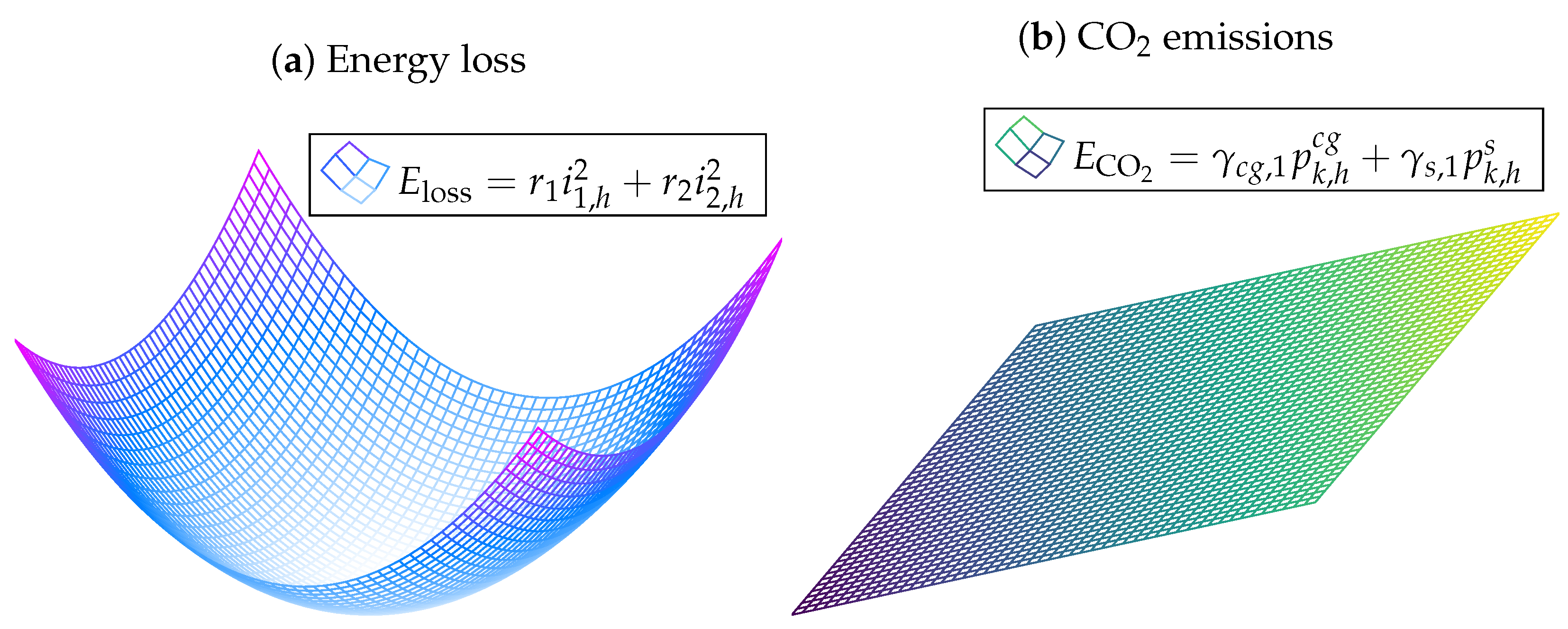
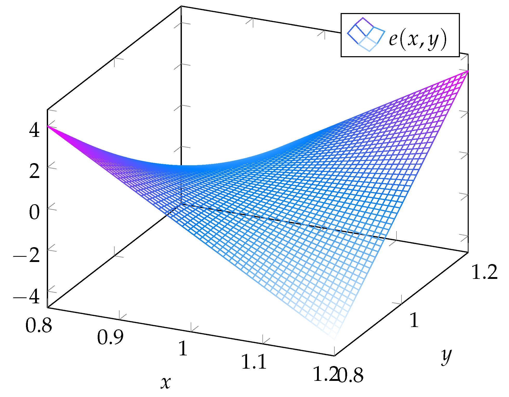
The three objective functions in (1)–(3) are from the family of convex functions, and are strictly convex, i.e., the energy losses since it is a hyper-paraboloid, while the energy purchasing costs are hyper-planes, i.e., convex and concave functions.

Let us present the general proof for these functions to confirm that all the objective functions are convex. A function is convex if the following inequality is fulfilled [26].

$$\begin{array}{c}\hfill f\left(\lambda x+\left(1-\lambda \right)y\right)\le \lambda f\left(x\right)+\left(1-\lambda \right)f\left(y\right).\end{array}$$

(12)

where $\lambda$ is a constant parameter defined between 0 and 1, and x and y are two points contained in the domain of the function under analysis.

a.

In the case of linear functions, let us consider a general form presented below.

$$\begin{array}{c}\hfill f\left(x\right)=\sum _{k\in \mathcal{K}}{C}_k{x}_k,\end{array}$$

(13)

where $C_k$ is a positive parameter, and considering the definition in (12), is obtained the following condition

$$\begin{array}{c}\hfill \sum _{k\in \mathcal{K}}{C}_k\lambda x_k+C_k\left(1-\lambda \right)y_k\le \lambda \sum _{k\in \mathcal{K}}{C}_k{x}_k+\left(1-\lambda \right)\sum _{k\in \mathcal{K}}{C}_k{x}_y.\end{array}$$

(14)

Note that in (14), is clear that the equality holds, ensuring that (13) is a convex function. Note that with this proof, functions (2) and (3) are confirmed as convex functions since both are linear functions with the form given by (13) [26].

b.

In the case of a quadratic function, let us consider a general form presented below.

$$\begin{array}{c}\hfill f\left(x\right)=\sum _{k\in \mathcal{K}}{D}_k{x}_k^2,\end{array}$$

(15)

where $D_k$ is a positive constant parameter. Now, considering the definition in (12), the following condition is obtained:

$$\begin{array}{c}\hfill \sum _{k\in \mathcal{K}}{D}_k{\left(\lambda x_k+\left(1-\lambda \right)y_k\right)}^2\le \lambda \sum _{k\in \mathcal{K}}{D}_k{x}_k^2+\left(1-\lambda \right)\sum _{k\in \mathcal{K}}{D}_k{y}_k^2,\end{array}$$

(16)

now, after applying some algebraic manipulations, the inequality condition in (16) can be reduced as follows:

$$\begin{array}{c}\hfill \sum _{k\in \mathcal{K}}{D}_k{\left(\lambda x_k+\left(1-\lambda \right)y_k\right)}^2\le \lambda \sum _{k\in \mathcal{K}}{D}_k{x}_k^2+\left(1-\lambda \right)\sum _{k\in \mathcal{K}}{D}_k{y}_k^2,\\ \hfill \sum _{k\in \mathcal{K}}{D}_k\left({\lambda }^2{x}_k^2+{\left(1-\lambda \right)}^2{y}_k^2+2\lambda \left(1-\lambda \right)x_k{y}_k\right)\le \lambda \sum _{k\in \mathcal{K}}{D}_k{x}_k^2+\left(1-\lambda \right)\sum _{k\in \mathcal{K}}{D}_k{y}_k^2,\\ \hfill \sum _{k\in \mathcal{K}}{D}_k\left(\left({\lambda }^2-\lambda \right)x_k^2+\left({\left(1-\lambda \right)}^2-\left(1-\lambda \right)\right)y_k^2+2\lambda \left(1-\lambda \right)x_k{y}_k\right)\le 0,\\ \hfill \sum _{k\in \mathcal{K}}{D}_k\left({\lambda }^2-\lambda \right)\left(x_k^2+y_k^2-2x_k{y}_k\right)\le 0,\\ \hfill \sum _{k\in \mathcal{K}}{D}_k\left({\lambda }^2-\lambda \right){\left(x_k+y_k\right)}^2\le 0,\end{array}$$

(17)

which clearly evidences that $\left({\lambda }^2-\lambda \right)\le 0$, and ${\left(x_k+y_k\right)}^2>0$ which implies that

$$\begin{array}{c}\hfill \sum _{k\in \mathcal{K}}{D}_k\left({\lambda }^2-\lambda \right){\left(x_k+y_k\right)}^2<0,\end{array}$$

(18)

Note that (18) is evidence that the quadratic function (15) is a strictly convex function, which confirms that the objective function (1) is also strictly convex [26].

The objective functions in (1) and (2) are illustrated in Figure 1 using a three-dimensional representation. The objective function regarding operating cost minimization is not plotted since it is also linear and contains three independent variables that cannot be plotted in a three-dimensional space.

ii.

The objective functions (2) and (3) are not two objectives in conflict since the minimization of one of them implies the minimization of the other one. This was recently demonstrated by authors of [11] for a single-objective analysis in grid-connected and stand-alone networks was made. In addition, they found that in the case of the objective function in (2), effectively, there is a conflicting behavior concerning the objectives in (2) and (3), respectively.

iii.

The set of constraints (5)–(11) is part of the linear affine and box-type constraints that are part of the convex set of constraints, which implies that these do not require any mathematical manipulation/approximation for convex optimization methods.

iv.

The only constraint that it is nonaffine in the optimization model (1)–(11) is the power balance constraint defined by (4) since it has multiple products between voltages and currents variables per node. In this research, to obtain a convex approximation of this set of equations, the McCormick approximation is used for the product of two variables.

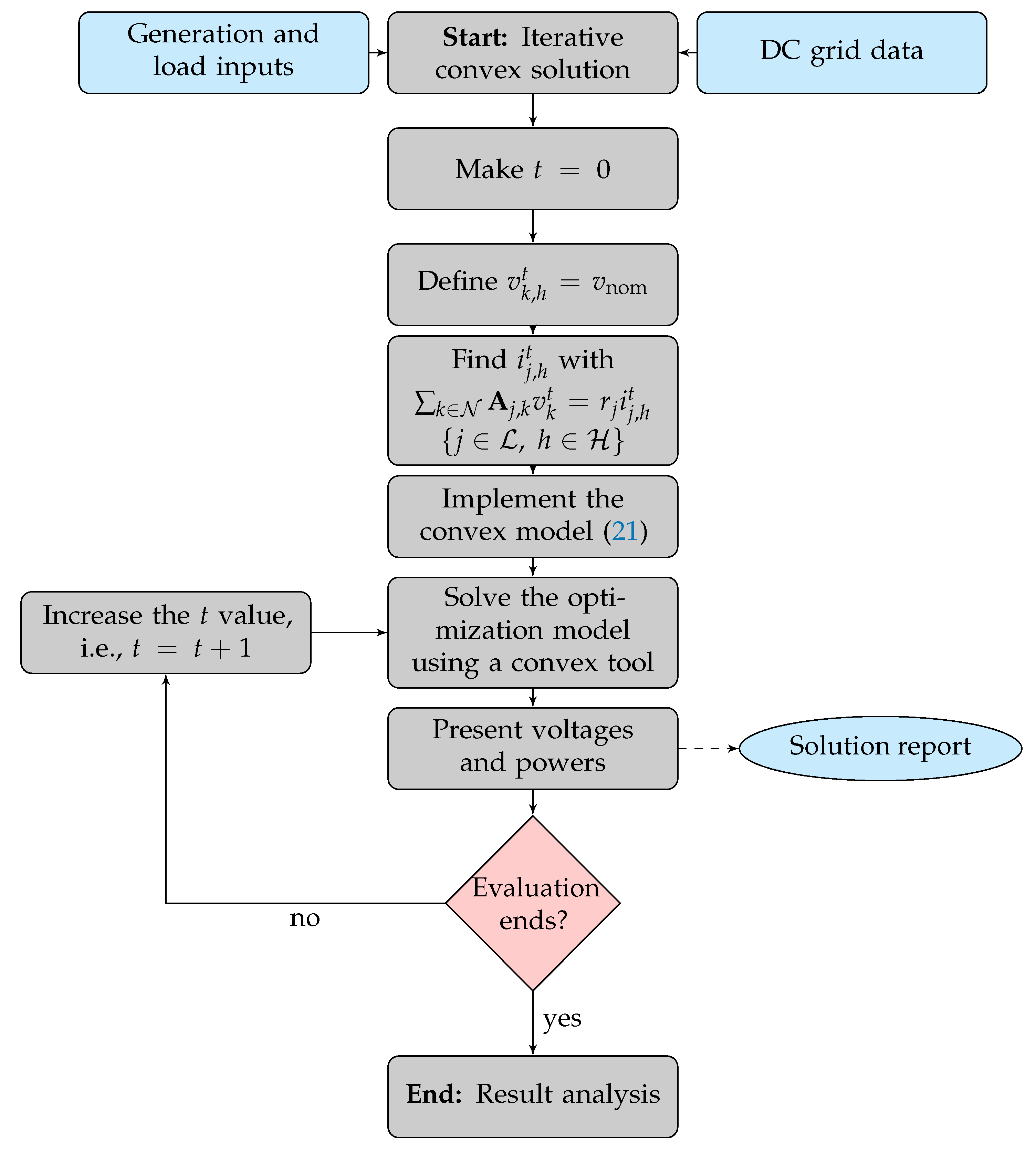
3. Proposed Solution Methodology

This section discusses the main characteristics of the proposed solution methodology, which is based on a convex approximation of the economic/technical/environmental day-ahead operation of PV plants in monopolar DC networks. In addition, a general iterative solution approach is presented to minimize the errors introduced during the convexification process.

3.1. Model Convexification

To obtain a linear equivalent formulation of the two variables, the McCormick approximation of two variables is implemented [27,28]. This approximation considers that the product of two continuous variables $f\left(x,y\right)=xy$ can be approximated as a linear equivalent function with the structure of (19).

$$\begin{array}{c}\hfill f\left(x,y\right)\approx y_{0}x+x_{0}y-y_0{x}_0,\end{array}$$

(19)

where $\left(x_0,y_0\right)$ is the linearization point. To illustrate the effect of the linearization method, let us define the error function $e\left(x,y\right)=100\left(xy-y_{0}x-x_{0}y+y_0{x}_0\right)$, which is plotted in Figure 2 considering that the linearizing point $\left(x_0,y_0\right)=\left(1,1\right)$.

Note that in the area of interest, i.e., in the neighborhood of $\left(x_0,y_0\right)$, the maximum estimation error between the exact and the approximated functions for the product of two variables is about $4\%$, can be considered acceptable due to voltage regulation constraints, this error will be lower since $v^{min}$ and $v^{max}$ are defined as 0.90 pu and 1.10 pu, which will limit the movements of the voltage variable in the power balance constraint more.

Remark 1.

Considering the linear approximation for the product of two variables in (19), the set of power balance constraints in (4) can be approximated as an affine set of constraints with the structure (20).

$$\begin{array}{c}\hfill p_{k,h}^{cg}+p_{k,h}^s+p_{k,h}^{pv}-p_{k,h}^d=\sum _{j\in \mathcal{L}}{\mathbf{A}}_{jk}\left(v_{k,h}^0{i}_{j,h}+i_{j,h}^0{v}_{k,h}-v_{k,h}^0{i}_{j,h}^0\right),\left\{k\in \mathcal{N},h\in \mathcal{H}\right\}\end{array}$$

(20)

where $v_{k,h}^0$ and $i_{j,h}^0$ are the linearizing points representing the initial values set for the voltage and currents.

3.2. Iterative Solution Approach

To minimize the error introduced by the convexification approach using the McCormick approximation for the product of two variables, we present an iterative counter t to represent the current values of the model variables ($x^t$) that serve to determine the new values of these represented with $t+1$, i.e., $x^{t+1}$. The general convex approximation model for the multi-objective problem of the optimal operation of PV plants considering economic, technical, and environmental objective functions is presented in (21)

$$\begin{array}{ccc}\hfill \mathrm{O}.\mathrm{F}.:& \hfill \hfill & \hfill \\ \hfill & min{E}_{\mathrm{loss}}=\sum _{h\in \mathcal{H}}\sum _{j\in \mathcal{L}}{r}_{km}{\left(i_{j,h}^{t+1}\right)}^2{\Delta }_h,\hfill & \hfill \\ \hfill & min{E}_{{\mathrm{CO}}_2}=\sum _{h\in \mathcal{H}}\sum _{k\in \mathcal{N}}\left({\gamma }_{cg,k}{p}_{k,h}^{cg}+{\gamma }_{s,k}{p}_{k,h}^s\right){\Delta }_h,\hfill & \hfill \\ \hfill & min{E}_{\cos \mathrm{ts}}=\sum _{h\in \mathcal{H}}\sum _{k\in \mathcal{N}}\left(C_{kWh}^{cg}{p}_{k,h}^{cg}+C_{kWh}^s{p}_{k,h}^s+C_{O\&M}^{pv}{p}_{k,h}^{pv}\right){\Delta }_h,\hfill & \hfill \end{array}$$

(21)

$$\begin{array}{ccc}\hfill \mathrm{s}.\mathrm{t}.:& \hfill \hfill & \hfill \\ \hfill & p_{k,h}^{cg}+p_{k,h}^s+p_{k,h}^{pv}-p_{k,h}^d=\sum _{j\in \mathcal{L}}{\mathbf{A}}_{jk}\left(v_{k,h}^t{i}_{j,h}^{t+1}+i_{j,h}^t{v}_{k,h}^{t+1}-v_{k,h}^t{i}_{j,h}^t\right),\hfill & \hfill \left\{k\in \mathcal{N},h\in \mathcal{H}\right\}\\ \hfill & \sum _{k\in \mathcal{N}}{\mathbf{A}}_{j,k}{v}_k^t=r_j{i}_{j,h}^t,\hfill & \hfill \left\{j\in \mathcal{L},h\in \mathcal{H}\right\}\\ \hfill & \sum _{k\in \mathcal{N}}{{\mathbf{A}}_{j,k}{v}_k}^{t+1}=r_j{i}_{j,h}^{t+1},\hfill & \hfill \left\{j\in \mathcal{L},h\in \mathcal{H}\right\}\\ \hfill & p_{k,h}^{cg,min}\le p_{k,h}^{cg}\le p_{k,h}^{cg,max},\hfill & \hfill \left\{k\in \mathcal{N},h\in \mathcal{H}\right\}\\ \hfill & p_{k,h}^{s,min}\le p_{k,h}^s\le p_{k,h}^{s,max},\hfill & \hfill \left\{k\in \mathcal{N},h\in \mathcal{H}\right\}\\ \hfill & p_{k,h}^{pv,min}\le p_{k,h}^{pv}\le p_{k,h}^{pv,max},\hfill & \hfill \left\{k\in \mathcal{N}.h\in \mathcal{H}\right\}\\ \hfill & -i_j^{max}\le i_{j,h}^{t+1}\le i_j^{max},\hfill & \hfill \left\{j\in \mathcal{L},h\in \mathcal{H}\right\}\\ \hfill & v^{min}\le v_{k,h}^{t+1}\le v^{max},\hfill & \hfill \left\{k\in \mathcal{N},h\in \mathcal{H}\right\}\\ \hfill & v_{k,h}^{t+1}=v_{k,h}^t=v_{\mathrm{nom}},\hfill & \hfill \left\{k=\mathrm{slack},h\in \mathcal{H}\right\}\end{array}$$

To recursively solve the approximated convex model (21) from the initial operative point (21), the flow chart in Figure 3 is employed.

To define if the iterative solution approach of the optimization model (21) presented in Figure 3 converges to the optimal solution, the following stopping criterion is applied.

$$\begin{array}{c}\hfill \underset{k\in \mathcal{N},h\in \mathcal{H}}{max}\left\{\left|v_{k,h}^{t+1}-\left|v_{k,h}^t\right|\right|\right\}\le \epsilon ,\end{array}$$

(22)

where $\epsilon$ is the assigned tolerance, which takes a value of $\epsilon =1\times {10}^{-8}$.

3.3. Multi-Objective Optimization Based on the Weight-Based Method

The weight-based optimization approach is implemented to obtain the Pareto front for the optimization problem defined in (21). Due to the multi-objective behavior between objective functions (1) and (2), and the objective functions (1) and (3), and the linear behavior between objective functions (2) and (3), in this research, a bi-dimensional multi-objective approach is implemented.

The general representation of the weight-based method for minimizing functions in (21) is the following:

$$\begin{array}{cc}\hfill \mathrm{Objective}\mathrm{function}& \hfill \hfill \\ \hfill & minz=\omega f_1\left(x\right)+\left(1-\omega \right)f_2\left(x\right),\hfill \\ \hfill \mathrm{Subject}\mathrm{to}& \hfill \hfill \\ \hfill & h\left(x\right)=0,\hfill \\ \hfill & g\left(x\right)\le 0,\hfill \\ \hfill & \omega \in \left[{\omega }^{min},{\omega }^{max}\right],\hfill \\ \hfill & x\in \left[x^{min},x^{max}\right],\hfill \end{array}$$

(23)

where $f_1\left(x\right)$ and $f_2\left(x\right)$ are two objective functions in conflict, $\omega$ is the weighing factor, z is the weighted-based objective function under minimization, $h\left(x\right)$ is the set of equality constraints, $g\left(x\right)$ is the set of inequality constraints, ${\omega }^{min}$ and ${\omega }^{max}$ are the lower and upper bounds set for the weighting factor, typically between 0 and 1, and $x^{min}$ and $x^{max}$ are the lower and upper bounds of the set of decision variables in the vector x.

Remark 2.

Observe that if objective functions $f_1\left(x\right)$ and $f_2\left(x\right)$ are two convex functions, then, the objective function z is also a convex function for $\omega \in \left[0,1\right]$, with ω being a predefined constant parameter. In addition, the solution of the weighted-based optimization model is carried out by sweeping some values of the ω factor in its feasible interval.

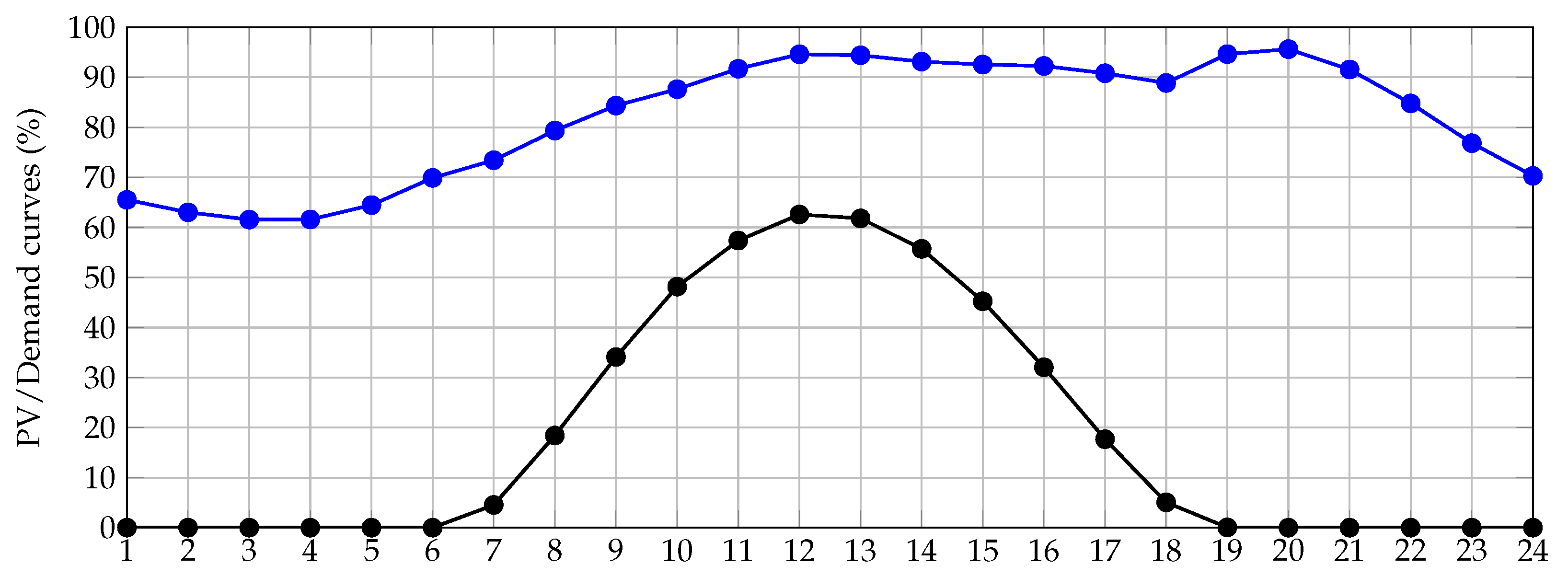
4. Distribution Network under Analysis

To validate the iterative convex solution for the recursive convex modeling in (21) via the flow diagram in Figure 3 considering the weighted-based multi-objective approach in (23), we considered the IEEE 33-bus grid in its DC version, which is depicted in Figure 4. It is worth mentioning that this test feeder was conditioned with information regarding demand profile and PV generation for the Medellín municipality in Colombia, as reported by the authors of [11].

For this test feeder, the following characteristics are presented:

i.

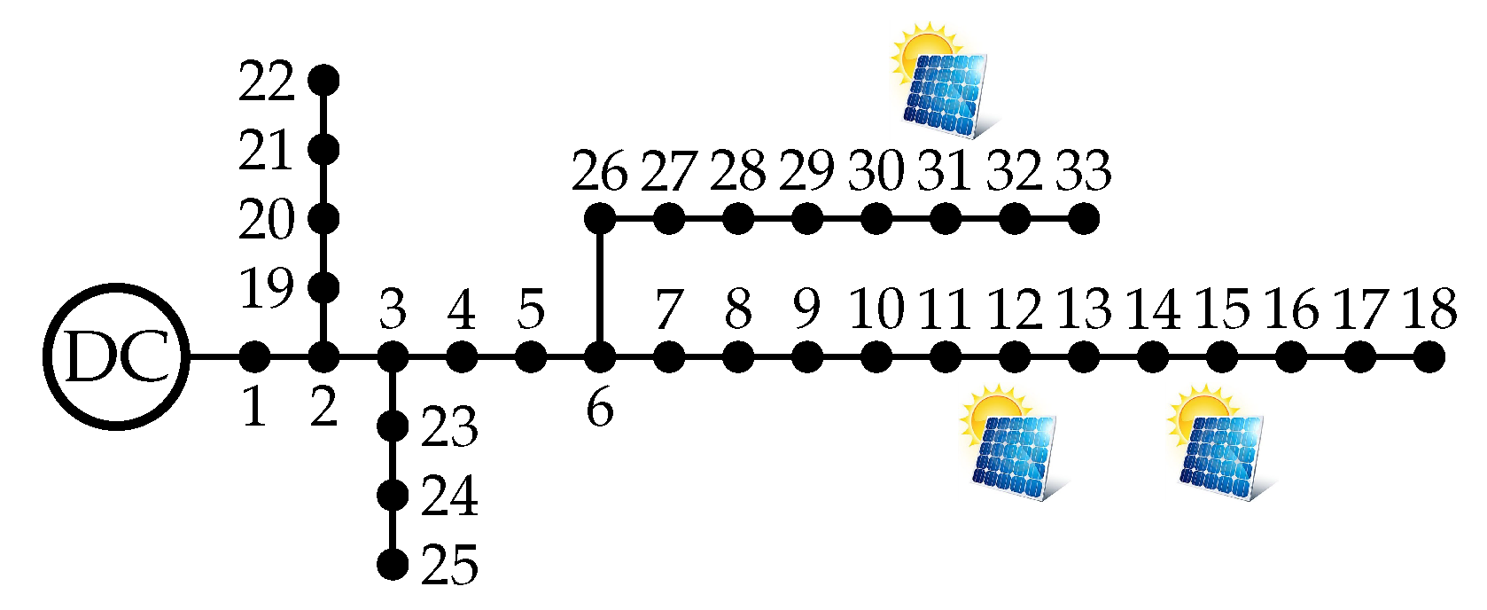
The operative voltage in terminals of the substation is 12.66 kk, i.e., this is a medium-voltage distribution network.

ii.

The electrical configuration of the IEEE 33-bus grid is radial, i.e., the number of branches is equal to the number of nodes minus one.

iii.

Three PV plants are previously installed at nodes 12, 15, and 31, all with the capacity of generating 2400 kW under nominal operation ratings.

All the parametric information related to loads and branches for this test feeder is presented in

Table 1. Network data regarding branches and loads.

Line l	Node i	Node j	${\mathit{R}}_{\mathbf{ij}}(\Omega )$	${\mathit{P}}_{\mathit{j}}$(kW)	${\mathit{I}}_{\mathit{l}}^{max}$(A)
1	1	2	0.0922	100	320
2	2	3	0.4930	90	280
3	3	4	0.3660	120	195
4	4	5	0.3811	60	195
5	5	6	0.8190	60	195
6	6	7	0.1872	200	95
7	7	8	1.7114	200	85
8	8	9	1.0300	60	70
9	9	10	1.0400	60	55
10	10	11	0.1966	45	55
11	11	12	0.3744	60	55
12	12	13	1.4680	60	40
13	13	14	0.5416	120	40
14	14	15	0.5910	60	25
15	15	16	0.7463	60	20
16	16	17	1.2890	60	20
17	17	18	0.7320	90	20
18	2	19	0.1640	90	30
19	19	20	1.5042	90	25
20	20	21	0.4095	90	20
21	21	22	0.7089	90	20
22	3	23	0.4512	90	85
23	23	24	0.8980	420	70
24	24	25	0.8900	420	40
25	6	26	0.2030	60	85
26	26	27	0.2842	60	85
27	27	28	1.0590	60	70
28	28	29	0.8042	120	70
29	29	30	0.5075	200	55
30	30	31	0.9744	150	40
31	31	32	0.3105	210	25
32	32	33	0.3410	60	20

.

To emulate the expected behavior regarding generation and demand for the IEEE 33-bus grid, the information presented by the authors of [11] is considered to set these parameters, which corresponds to the data for Medellín city. The percentage of demand and the expected PV generation profiles are depicted in Figure 5.

5. Numerical Validations

Here are all the numerical results on the IEEE 33-bus grid in its DC version. For this computational implementation, the MATLAB programming environment, version 2021b, was used on a PC with an AMD Ryzen 7 3700 $2.3$ GHz processor and 16.0 GB RAM used running on a 64-bit version of Microsoft Windows 10 Single Language. The solution of the recursive convex approximation (21) was reached in the convex disciplined tool environment (known as CVX) for MATLAB using the SEDUMI and SDPT3 solvers.

The following simulation scenarios are considered to validate the effectiveness of the convex optimization methodology in dealing with the problem of optimal operation of PV plants in monopolar DC networks.

i.

A comparative analysis with different metaheuristic optimization methods is presented using a single-objective minimization analysis.

ii.

The construction of the Pareto fronts for the pairs technical-economic and environmental-economic is presented.

Table 2. Parametrization of the objective function.

Parameter	Value	Unit
${\gamma }_{cg}$	0.2671	kg/kWh
${\gamma }_s$	0.1644	kg/kWh
$C_{kWh}^{cg}$	0.2913	USD/kWh
$C_{kWh}^s$	0.1302	USD/kWh
$C_{O\&M}^{pv}$	0.0019	USD/kWh

lists all the parameters to evaluate the objective functions. These data have been adapted from [11].

5.1. Single-Objective Function Analysis

This section is considered a single-objective function analysis to demonstrate the effectiveness of the proposed iterative solution methodology (ahead, ISM) in operating PV plants in monopolar DC networks. For comparative purposes, four different optimization algorithms from the family of metaheuristics optimizers recently reported by authors of [11] are considered. These algorithms are the crow search algorithm (CSA), the particle swarm optimizer (PSO), the multiverse optimizer (MVO), and the salp swarm algorithm (SSA). It is worth mentioning that each one of these optimizers was evaluated 100 times to determine their average behavior regarding the objective function minimization. Comparative results between the metaheuristic optimizers and the proposed ISM are presented in

Table 3. Comparative analysis of the combinatorial methods with the proposed ISM.

Method	E${}_{\mathbf{loss}}$ (kWh/day)	E${}_{\mathbf{costs}}$ (USD/day)	E${}_{{\mathbf{CO}}_2}$ (kg/day)
Benc. Case	2186.2803	9776.3892	12,345.1497
CSA	1270.1562	7407.9046	9328.7685
PSO	1268.5973	7392.0432	9282.4081
MVO	1231.2531	7298.7157	9187.9682
SSA	1225.3323	7297.9712	9166.6746
ISM	1224.8548	7137.1822	8965.4072

.

The numerical results in Table 3 reveal that:

i.

The best combinatorial optimization method corresponds to the SSA since it finds the best numerical solution of each objective function when compared with the remainder of metaheuristic optimizers. In the case of the energy losses minimization, it finds a reduction of about $960.9480$ kWh/day concerning the benchmark case; when is minimized the total energy purchasing and operating costs, the reduction with the SSA approach was about USD $2478.418$ per day of operation. Finally, when it is minimized the total emissions of CO${}_2$, the SSA approach reduces the objective function by about $3178.4751$ kg/day.

ii.

The CSA, PSO, and MVO found important reductions concerning the benchmark case of each objective function minimization; however, they all stay stuck in locally optimal solutions. Note that the minimum reductions with respect to each objective function were provided by the CSA with values of $41.9033\%$ (energy losses), $24.2265\%$ (energy costs), and $24.4337$ (CO${}_2$ emissions). In contrast, the maximum reductions were found with the SSA approaches, being these $43.9535\%$, $25.3511\%$, and $5.7467\%$, respectively.

iii.

The proposed ISM found the best solution values for each objective function in the single-objective function analysis, i.e., the globally optimal solution (these were corroborated with the solution of the exact NLP model in the GAMS software [29]). When energy losses are minimized, the daily reduction is about $961.4255$ kWh/day, i.e., $43.9754\%$. In the case of the minimization of energy purchasing costs, a reduction of USD $2639.2070$ per day of operation, i.e., a reduction of $26.9957\%$, was found. Finally, when the CO${}_2$ emissions are minimized, the ISM found a reduction of about $3379.74250$ kg/day, corresponding to a reduction of $27.3771\%$.

iv

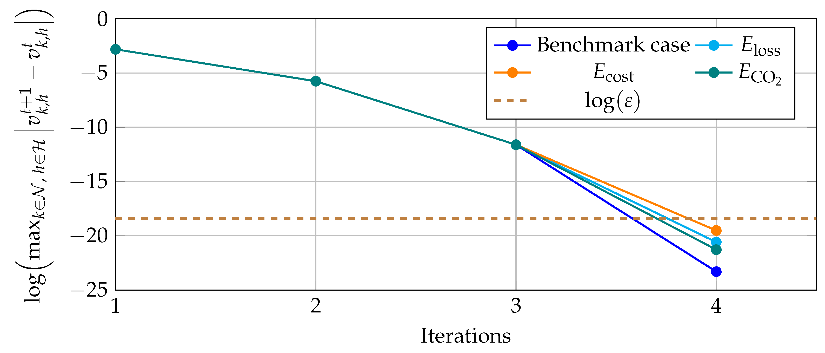
When the SSA approach and the ISM are compared, it is observed that for each one of the objective functions, the ISM finds better numerical reductions. These improvements are $0.4775$ kWh/day, USD $160.7790$ per day of operation, and $201.2674$ kg/day, respectively. Nevertheless, the most important result in Table 3 is that owing to the convex nature of the solution space and objective function in (21), the ISM always finds the same objective function value for each one of the objectives; however, it is not possible with each running of the SSA approach due to its random nature and nonconvexity of the original NLP model (1)–(11).

To observe the effect of the McCormick approximation of the product between two positive variables that allowed to obtain an approximated affine equivalent for the power balance constraint (4) as presented in (20) is used Figure 6, where the convergence characteristic of the proposed recursive convex optimization model considering the expected estimation error and the number of solution to reach the desired tolerance (i.e., $\epsilon =1\times {10}^{-8}$).

Note that the behavior in Figure 6 shows that: (i) the McCormick approximation for each of the single-objective function analysis, including the benchmark case, reach the expected convergence error after four iterations, i.e., it is possible to affirm that after four iterations, the error introduced by the McCormick linearization is negligible, and the solution of each objective function reaches the optimal value (see results in Table 3); (ii) the convergence of the proposed recursive approximation methodology is quadratic, which confirms the nature of the derivative-based approximation as the case of the McCormick approximation (linear approximation of the product of two variables using Taylor’s series expansion) which in the Newton–Raphson case exhibits quadratic convergence (for more details regarding the convergence of power flow methods, see reference [30]).

To confirm that the solution of each objective function with the ISM is feasible, Figure 7 depicts the daily variation of the loadability of each distribution line. The loadability is calculated as the current flow over the maximum thermal bound for each line in Table 1 at each analysis period.

The main characteristics in Figure 7 are that for the benchmark case, any distribution line is operating with 100% of current transference capability as observed in Figure 7a, and that there are some periods of operation where some distribution lines are loaded at 100%. This is the case of branch 30 when the minimization is applied to the daily energy loss function (see Figure 7b). In the case of the energy purchasing costs minimization, the lines that operate with 100% of loadability are 11, 14, and 30, as can be seen in Figure 7c. While minimizing the amount of CO${}_2$ emissions, the saturated branches are 11 and 30 (see Figure 7d). However, two main conclusions can be obtained from these plots: (i) all the operative constraints in the optimization model are fulfilled, i.e., the final results in Table 3 are 100% feasible; (ii) the lines with saturation are distribution lines located directly in the area of influence of the PV plants, which will have significant changes in their current flows when the PV generation increases considerably.

5.2. Sensitivity Analysis

To evaluate the effect of the power generation variability and expected demand profile in the expected behavior of the objective function values, here we present a sensitivity analysis regarding possible variations from the PV generation sources from 75% to 105% of energy availability in these sources by maintaining the demand curve fixed. In addition, the generation curve is fixed by varying the expected demand consumption between 75% and 105% of its nominal value.

Table 4. Sensitivity analysis regarding variations in the power generation availability and demand behavior (all values are per day of operation).

PV (%)	E${}_{\mathbf{loss}}$ (USD)	E${}_{{\mathbf{CO}}_2}$ (kg)	E${}_{\mathbf{costs}}$ (USD)	Dem. (%)	E${}_{\mathbf{loss}}$ (USD)	E${}_{{\mathbf{CO}}_2}$ (kg)	E${}_{\mathbf{costs}}$ (USD)
75	1258.5109	9191.5059	7313.6805	75	664.1192	6130.7524	4889.5067
80	1250.0079	9134.9309	7269.5171	80	761.3790	6693.2993	5335.5873
85	1242.5269	9088.8165	7233.5176	85	865.8561	7257.2783	5782.8021
90	1235.8723	9047.5459	7201.2994	90	977.7199	7824.5048	6232.5675
95	1230.0092	9006.4100	7169.1879	95	1097.3414	8394.2082	6684.2826
100	1224.8548	8965.4072	7137.1822	100	1224.8548	8965.4072	7137.1822
105	1220.2060	8924.5361	7105.2808	105	1360.5354	9538.1184	7591.2792

presents the behavior of each objective function when the single-objective function analysis is applied. It is essential to mention that for demand increments higher than 105%, the studied problem is infeasible due to the thermal constraints imposed by the conductors.

The numerical results in Table 4 reveal that:

i.

The effect of renewable generation availability on all the objective function values is minimal since differences between generation availability between 75%, and 105% are about $38.3049$ kWh/day, $266.9698$ kg/day, and $208.3997$ USD/day. These small differences are attributable to the fact that PV generations are optimally dispatched without applying the maximum power point tracking point, i.e., that the energy used from these sources is a function of the grid requirements. In addition, it can also indicate that the size of the batteries is small, and these can not take advantage of the total renewable energy resource available.

ii.

As expected, the behavior of the demand profile has highly influenced all the objective functions analyzed since the energy losses, generation costs, and greenhouse gas emissions are a function of the total grid power consumption. Note that variations of these objective functions when the PV generation is maintained at 100% and the demand varies from 875% to 105% are $696.4162$ kWh/day, $3407.3660$ kg/day, and $2701.7725$ USD/day.

The behavior of the $E_{{\mathrm{CO}}_2}$ vs. $E_{\mathrm{costs}}$ shows that the minimization of each one of these objectives implies the minimization of the other one. This confirms that both objectives are linearly dependent and are not in conflict. This is attributable to the fact that functions (2) and (3) are linear functions of the power generation output in the substation terminal with positive coefficients, which implies that the same combination of variables minimizes both objectives simultaneously. More details regarding this behavior of $E_{{\mathrm{CO}}_2}$ vs. $E_{\mathrm{costs}}$ will be discussed below.

5.3. Multi-Objective Analysis

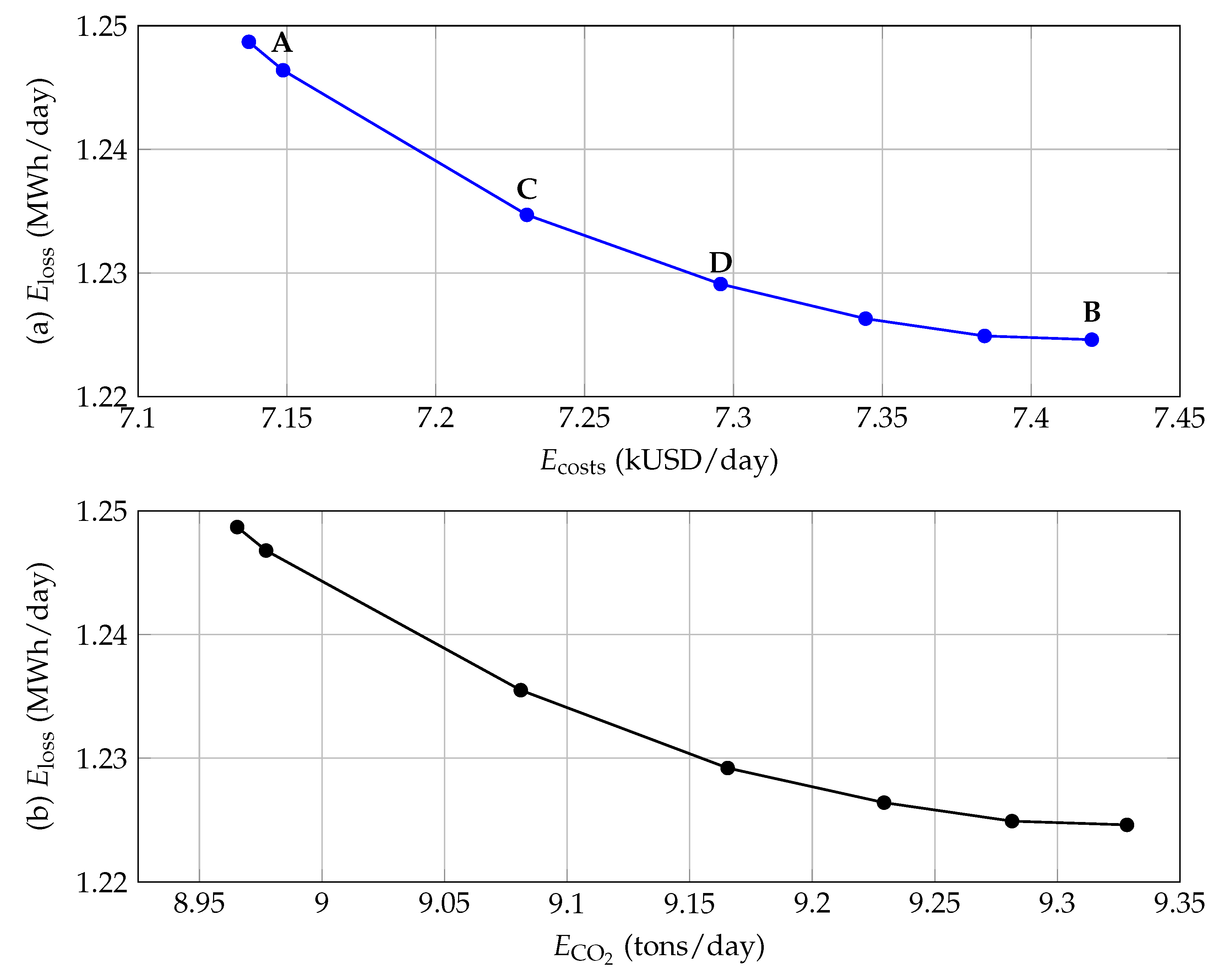
In this section, the weighted-based multi-objective approach presented in (23) is applied for pairs of objective functions. For constructing the Pareto front of each pair of objective functions, the parameter $\omega$ sweeps between 0 and 1 in steps of 0.1. Figure 8 presents the Pareto front for the pair of objective functions $E_{\mathrm{costs}}$ vs. $E_{\mathrm{loss}}$, and $E_{{\mathrm{CO}}_2}$ vs. $E_{\mathrm{loss}}$.

The behavior of the Pareto fronts in Figure 8 shows that both Pareto fronts, i.e., $E_{\mathrm{costs}}$ vs. $E_{\mathrm{loss}}$ in Figure 8a and $E_{\mathrm{costs}}$ vs. $E_{{\mathrm{CO}}_2}$ in Figure 8b have the same behavior, i.e., the points associated with the upright axis are the same in both fronts, there is only a modification of the scale in the horizontal axis. This behavior in both fronts confirms that the $E_{\mathrm{costs}}$ and the $E_{{\mathrm{CO}}_2}$ are functions that when one of them is minimized the other one is also minimized as well.

Table 5. Data of the market points for the Pareto front Figure 8a.

Point	E${}_{\mathbf{loss}}$ (kWh/day)	E${}_{\mathbf{costs}}$ (USD/day)	E${}_{{\mathbf{CO}}_2}$ (kg/day)
A	1248.7029	7137.1922	8965.4072
C	1235.5288	7227.4401	9081.1005
D	1229.1622	7293.2576	9165.4578
B	1224.5628	7420.4024	9328.3993

presents the values for all the market points in Figure 8a, which correspond to the extreme values (points A and B), and the central values in the case of points C and D.

The numerical results in Table 5 show that:

i.

The extreme point A represents the maximum value of the energy losses during the daily operation with a value of $1248.7029$ kWh/day, being the minimum value for the energy purchasing costs and the CO${}_2$ emissions with values of USD /day $7137.1922$ and kg/day $8965.4072$, respectively. Note that these points are the optimal solution when the $E_{\mathrm{costs}}$ and $E_{{\mathrm{CO}}_2}$ are minimized using the single-objective analysis as presented in Table 3 for the ISM approach.

ii.

The extreme point B represents the minimum value possible for the total daily energy losses reduction, i.e., $1224.5628$ kWh/day, and at the same time, the maximum value for the total grid operative costs and the greenhouse gas emissions, with values of USD /day $7420.4024$ and kg/day $9328.3993$. Note that this point is the optimal solution when the energy loss is considered in the single-objective function analysis (see Table 3 for the ISM approach).

iii.

The difference between the extreme points A and B regarding each one of the objective functions where kWh/day $24.1401$, USD/day $283.2102$, and kg/day $362.9921$, per day of operation, which means that depending on the objective function selected by the distribution company to operate each network, one of them will benefit to the detriment of the others. However, if points C or D are selected as operative points, these can balance the reduction in all the objective functions with adequate minimization in all the objective functions with respect to their maximums.

6. Conclusions and Future Work

The problem of the efficient dispatch of PV plants in monopolar DC distribution networks was addressed in this research using a convex approximation procedure. Three objective functions were considered in the mathematical formulation: minimization of the daily energy losses, energy purchasing combined with maintenance costs in PV plants, and the total emissions of CO${}_2$. The convexification of the exact NLP model was made through the McCormick equivalent of the product between two continuous variables. To reduce the estimation error introduced by the McCormick approximation, an iterative solution methodology was proposed by starting with plane voltages (equal magnitudes to the substation bus) in all the network nodes. The main advantage of the proposed McCormick approximation is that it ensures quadratic convergence to the global solution, which, as expected, is based on derivatives that, as in the case of the Newton-based approaches, converge quadratically in power flow problems in DC networks.

To validate the effectiveness of the proposed ISM, two simulations were evaluated in the DC version of the IEEE 33-bus grid. The first simulation corresponded to the minimization of each objective function individually. The second approach was the application of the weighted-based optimization method to obtain the Pareto front for two pairs of functions ($E_{\mathrm{loss}}$ vs. $E_{\mathrm{costs}}$) and ($E_{\mathrm{loss}}$ vs. $E_{{\mathrm{CO}}_2}$). In addition, it was demonstrated that the pair $E_{\mathrm{costs}}$ vs. $E_{{\mathrm{CO}}_2}$ is not a set of conflicting functions, i.e., the minimization of one of them also implies the minimization of the other one. The main advantage of having a Pareto front is that there is a set of possibilities for optimal operation of PV plants as a function of the interest of the distribution company, which is not the case of the single-objective function analysis, where the minimization of one of the objective functions will affect the expected reductions in the other objective in conflict.

In the case of the single-objective function analysis, the proposed ISM demonstrated that it could deal with the minimization of each objective function and finds the optimum global value. Its efficiency was compared with multiple combinatorial optimizers. The SSA approach was the most efficient metaheuristic approach; however, this algorithm stayed stuck in locally optimal solutions compared with the proposed ISM. The common characteristic between the single- and multi-objective function approaches is that the extreme solutions in the Pareto front correspond to the optimal solutions in the single-objective function analysis. These coincidences confirm that the ICS methodology can effectively reach the best possible solution for the studied problem even if single- and multi-objective approaches are implemented.

Sensitivity analysis regarding the variations in the PV generation availability and expected demand consumption showed that in the former case, there are small variations in all the objective function values, which means that the renewable energy availability is enough to cover all the grid requirements if it is upper than 75%; however, the variations in the demand profile, as expected, had important effects in the final objective function values, which is explained by the fact that the energy losses is a square function of the total consumption and the operating costs and greenhouse gas emissions are linear functions of the load profile, respectively.

Possible future works derived from this research are the following: (i) a complete comparative analysis between convexification techniques, i.e., second-order cone programming, semidefinite programming, and recursive convex methods; (ii) the extension of the proposed ISM to the operation of monopolar DC networks with different renewable generation sources and battery energy storage systems; (iii) the inclusion of uncertainties in the generation and demand profiles using robust convex optimization; (iv) the improvement of the battery modeling to include aging-aware degradation characteristics in these elements.

References

1. Garces, A. On the Convergence of Newton’s Method in Power Flow Studies for DC Microgrids. IEEE Trans. Power Syst. 2018, 33, 5770–5777. [Google Scholar] [CrossRef] [Green Version]
2. Xu, Y.; Hu, Z.; Ma, T. Monopolar Grounding Fault Location Method of DC Distribution Network Based on Improved ReliefF and Weighted Random Forest. Energies 2022, 15, 7261. [Google Scholar] [CrossRef]
3. Gan, L.; Low, S.H. Optimal Power Flow in Direct Current Networks. IEEE Trans. Power Syst. 2014, 29, 2892–2904. [Google Scholar] [CrossRef]
4. Garces, A. Uniqueness of the power flow solutions in low voltage direct current grids. Electr. Power Syst. Res. 2017, 151, 149–153. [Google Scholar] [CrossRef]
5. Li, J.; Liu, F.; Wang, Z.; Low, S.H.; Mei, S. Optimal Power Flow in Stand-Alone DC Microgrids. IEEE Trans. Power Syst. 2018, 33, 5496–5506. [Google Scholar] [CrossRef] [Green Version]
6. Kumar, A.A.; Prabha, N.A. A comprehensive review of DC microgrid in market segments and control technique. Heliyon 2022, 8, e11694. [Google Scholar] [CrossRef]
7. Shahradfar, E.; Fakharian, A. Optimal controller design for DC microgrid based on state-dependent Riccati Equation (SDRE) approach. Cyber-Phys. Syst. 2020, 7, 41–72. [Google Scholar] [CrossRef]
8. El-Ela, A.A.; Mosalam, H.A.; Amer, R.A. Optimal control design and management of complete DC- renewable energy microgrid system. Ain Shams Eng. J. 2022, 14, 101964. [Google Scholar] [CrossRef]
9. Sabzian-Molaee, Z.; Rokrok, E.; Doostizadeh, M. An optimal planning model for AC-DC distribution systems considering the converter lifetime. Int. J. Electr. Power Energy Syst. 2022, 138, 107911. [Google Scholar] [CrossRef]
10. Serra, F.M.; Montoya, O.D.; Alvarado-Barrios, L.; Álvarez-Arroyo, C.; Chamorro, H.R. On the Optimal Selection and Integration of Batteries in DC Grids through a Mixed-Integer Quadratic Convex Formulation. Electronics 2021, 10, 2339. [Google Scholar] [CrossRef]
11. Grisales-Noreña, L.F.; Ocampo-Toro, J.A.; Rosales-Muñoz, A.A.; Cortes-Caicedo, B.; Montoya, O.D. An Energy Management System for PV Sources in Standalone and Connected DC Networks Considering Economic, Technical, and Environmental Indices. Sustainability 2022, 14, 16429. [Google Scholar] [CrossRef]
12. Montoya, O.D.; Grisales-Noreña, L.F.; Gil-González, W.; Alcalá, G.; Hernandez-Escobedo, Q. Optimal Location and Sizing of PV Sources in DC Networks for Minimizing Greenhouse Emissions in Diesel Generators. Symmetry 2020, 12, 322. [Google Scholar] [CrossRef] [Green Version]
13. Iris, Ç.; Lam, J.S.L. Optimal energy management and operations planning in seaports with smart grid while harnessing renewable energy under uncertainty. Omega 2021, 103, 102445. [Google Scholar] [CrossRef]
14. Iris, Ç.; Lam, J.S.L. A review of energy efficiency in ports: Operational strategies, technologies and energy management systems. Renew. Sustain. Energy Rev. 2019, 112, 170–182. [Google Scholar] [CrossRef]
15. Ferreira, J.; Afonso, J.; Monteiro, V.; Afonso, J. An Energy Management Platform for Public Buildings. Electronics 2018, 7, 294. [Google Scholar] [CrossRef] [Green Version]
16. Mariano-Hernández, D.; Hernández-Callejo, L.; Zorita-Lamadrid, A.; Duque-Pérez, O.; García, F.S. A review of strategies for building energy management system: Model predictive control, demand side management, optimization, and fault detect &diagnosis. J. Build. Eng. 2021, 33, 101692. [Google Scholar] [CrossRef]
17. Hohne, P.A.; Kusakana, K.; Numbi, B.P. Improving Energy Efficiency of Thermal Processes in Healthcare Institutions: A Review on the Latest Sustainable Energy Management Strategies. Energies 2020, 13, 569. [Google Scholar] [CrossRef] [Green Version]
18. Pereira, F.; Caetano, N.S.; Felgueiras, C. Increasing energy efficiency with a smart farm—An economic evaluation. Energy Rep. 2022, 8, 454–461. [Google Scholar] [CrossRef]
19. Zhuo, Z.; Zhang, N.; Kang, C.; Dong, R.; Liu, Y. Optimal Operation of Hybrid AC/DC Distribution Network with High Penetrated Renewable Energy. In Proceedings of the 2018 IEEE Power & Energy Society General Meeting (PESGM), Portland, OR, USA, 5–10 August 2018. [Google Scholar] [CrossRef]
20. LI, P.; Zheng, M. Multi-objective optimal operation of hybrid AC/DC microgrid considering source-network-load coordination. J. Mod. Power Syst. Clean Energy 2019, 7, 1229–1240. [Google Scholar] [CrossRef]
21. Gomez, A.L.; Arredondo, C.A.; Luna, M.A.; Villegas, S.; Hernandez, J. Regulating the integration of renewable energy in Colombia: Implications of Law 1715 of 2014. In Proceedings of the 2016 IEEE 43rd Photovoltaic Specialists Conference (PVSC), Portland, OR, USA, 5–10 June 2016. [Google Scholar] [CrossRef]
22. López, A.R.; Krumm, A.; Schattenhofer, L.; Burandt, T.; Montoya, F.C.; Oberländer, N.; Oei, P.Y. Solar PV generation in Colombia—A qualitative and quantitative approach to analyze the potential of solar energy market. Renew. Energy 2020, 148, 1266–1279. [Google Scholar] [CrossRef]
23. Rodríguez-Urrego, D.; Rodríguez-Urrego, L. Photovoltaic energy in Colombia: Current status, inventory, policies and future prospects. Renew. Sustain. Energy Rev. 2018, 92, 160–170. [Google Scholar] [CrossRef]
24. Molina, A.; Montoya, O.D.; Gil-González, W. Exact minimization of the energy losses and the CO2 emissions in isolated DC distribution networks using PV sources. Dyna 2021, 88, 178–184. [Google Scholar] [CrossRef]
25. Shen, T.; Li, Y.; Xiang, J. A Graph-Based Power Flow Method for Balanced Distribution Systems. Energies 2018, 11, 511. [Google Scholar] [CrossRef] [Green Version]
26. Garcés-Ruiz, A. Optimización Convexa, Aplicaciones en Operación y Dinámica de Sistemas de Potencia; Universidad Tecnológica de Pereira: Pereira, Colombia, 2020. [Google Scholar] [CrossRef]
27. Ferro, G.; Robba, M.; D’Achiardi, D.; Haider, R.; Annaswamy, A.M. A distributed approach to the Optimal Power Flow problem for unbalanced and mesh networks. IFAC-PapersOnLine 2020, 53, 13287–13292. [Google Scholar] [CrossRef]
28. Javadi, M.S.; Gouveia, C.S.; Carvalho, L.M.; Silva, R. Optimal Power Flow Solution for Distribution Networks using Quadratically Constrained Programming and McCormick Relaxation Technique. In Proceedings of the 2021 IEEE International Conference on Environment and Electrical Engineering and 2021 IEEE Industrial and Commercial Power Systems Europe (EEEIC/I&CPS Europe), Bari, Italy, 7–10 September 2021. [Google Scholar] [CrossRef]
29. Soroudi, A. Power System Optimization Modeling in GAMS; Springer International Publishing: Berlin/Heidelberg, Germany, 2017. [Google Scholar] [CrossRef]
30. Montoya, O.D.; Molina-Cabrera, A.; Hernández, J.C. A Comparative Study on Power Flow Methods Applied to AC Distribution Networks with Single-Phase Representation. Electronics 2021, 10, 2573. [Google Scholar] [CrossRef]
Figure 1. Convex structure of the objective functions: (a) hyper-paraboloid that represents the energy loss function in (1), and (b) plane that represents the emissions of CO 2 in (2).
Energies 16 00976 g001
Figure 2. Percentage of error between the exact and the linear approximation function for the product of two variables.
Energies 16 00976 g002
Figure 3. Iterative solution approach for the convex approximation model in (21).
Energies 16 00976 g003
Figure 4. Adaptation of the IEEE 33-bus grid for DC monopolar applications.
Energies 16 00976 g004
Figure 5. Graph of the electrical demand consumption and power generation with PV plants in Medellín, Colombia.
Energies 16 00976 g005
Figure 6. Evolution of the error in the proposed recursive approximation method for the benchmark case and the optimization of each single-objective function optimization.
Energies 16 00976 g006
Figure 7. Percentage of variation of the current at each distribution line at each period of analysis: (a) current behavior in the benchmark case (no PV plants connected); (b) current behavior when Eloss is minimized; (c) current behavior when Ecosts is minimized; (d) current behavior when ECO2 is minimized.
Energies 16 00976 g007aEnergies 16 00976 g007b
Figure 8. Pareto front for the conflicting objective functions: (a) E costs vs. E loss , and (b) E cos ts vs. E CO 2 .
Energies 16 00976 g008