Energy Production Analysis of Rooftop PV Systems Equipped with Module-Level Power Electronics under Partial Shading Conditions Based on Mixed-Effects Model

Abstract

The rooftop photovoltaic (PV) system that uses a power optimization device at the module level (MLPE) has been theoretically proven to have an advantage over other types in case of reducing the effect of partial shading. Unfortunately, there is still a lack of studies about the energy production of such a system in real working conditions with the impact of partial shading conditions (PSC). In this study, we evaluated the electrical energy production of the PV systems which use two typical configurations of power optimization at the PV panel level, a DC optimizer and a microinverter, using their real datasets working under PSC. Firstly, we compared the energy utilization ratio of the monthly energy production of these systems to the reference ones generated from PVWatt software to evaluate the effect of PSC on energy production. Secondly, we conducted a linear decline model to estimate the annual degradation rate of PV systems during a 6-year period to evaluate the effect of PSC on the PV’s degradation rate. In order to perform these evaluations, we utilized a mixed-effects model, a practical approach for studying time series data. The findings showed that the energy utilization ratio of PVs with MLPE was reduced by about $14.7\%$ ($95\%$ confidence interval: $-27.3\%$ to $-2.0\%$) under PSC, compared to that under nonshading conditions (NSC). Another finding was that the PSC did not significantly impact the PV’s annual energy degradation rate, which was about $-50$ (Wh/kW) per year. Our finding could therefore be used by homeowners to help make their decision, as a recommendation to select the gained energy production under PSC or the cost of a rooftop PV system using MLPE for their investment. Our finding also suggested that in the area where partial shading rarely happened, the rooftop PV system using a string or centralized inverter configuration was a more appropriate option than MLPE. Finally, our study provides an understanding about the ability of MLPE to reduce the effect of PSC in real working conditions.

1. Introduction

The rooftop photovoltaic (PV) system plays a crucial role in renewable energy resources in the residential domain of smart grid development. However, partial shading, which is caused by a range of issues such as trees, chimneys, or neighbor buildings, leads to the energy production losses. Reducing the impact of partial shading still requires a significant research effort in the system configuration to maximize the generated energy from the PV system [1,2,3,4,5,6,7,8,9]. Recently, the usage of module-level power electronics for PV systems, such as a DC optimizer and microinverter, has been shown to improve the energy harvesting of PV systems under PSC.

In a DC-optimizer-equipped PV, a DC power optimizer (e.g., SolarEdge inverter [10]) is integrated with the junction box of a PV panel to increase the energy production of the module before it transfers an optimized DC voltage to the central inverter of a centralized PV system (Figure 1 (left)). A DC optimizer is a DC-to-DC converter that performs MPPT at the module level. DC power optimizers deliver system benefits, including maintaining the energy performance under partial shading or other mismatch situations, low-voltage safety under emergency disconnect situations, and relaxed drawing constraints for the PV installer.

In a microinverter PV, the inverter (e.g., Enphase microinverter [11]) performs the same essential operation as a centralized inverter, that is, modifying direct current into alternating current, but it makes the conversion at the PV panel (Figure 1 (right)). Like the DC power optimizer, the microinverter allows the MPPT to increase the output of each solar panel to be unaffected by the other panels in the system. This feature contrasts with a centralized PV system in which the panels are connected in strings and wired to a central inverter. Microinverters can also improve the overall system’s AC output when a portion of the PV system must be installed on more than one roof plane or when the PV panels are unevenly shaded.

There has been a growing interest in evaluating the energy performance of PV systems equipped with MLPE under PSC in the literature. The NREL [12,13] conducted studies for estimating the energy performance of using MLPE under PSC based on real testing conditions for residential PV systems. The result of the annual energy recovery of shading losses was up from $25\%$ to $35\%$ compared to the string inverter configuration. The authors in [14,15] established an outdoor test comparing the string inverter and MLPE energy performance under NSC and PSC during a 6-month period. The results showed that MLPE increased the performance ratio up to $35\%$ under PSC, but the string system outperformed MLPE under NSC. In [16], the authors showed a better energy performance and energy production of a DC-optimizer PV system using a simulation of PSC and one week of data. In [17], the authors conducted a Matlab simulation of MLPE and a string inverter in PSC. The results found that MLPE were slightly better in PSC, but in NSC, it did not bring any advantages. In addition, the cost of MLPE was higher than that of the string inverter. The MLPE mismatch study at large-scale photovoltaic plants in [18] stated that the improvement of energy production was still a consideration compared to the string or centralized PV systems equipped with MPPT. Finally, the analysis in [19] across a total of 542 Tigo Energy’s DC power optimizers found a mean power loss of $8.3\%$ due to PSC, which would have increased to $13\%$ were the PVs not equipped with panel-level optimizers. It was estimated that on average, about $36\%$ of the power loss from partial shading was regained through the use of MLPE.

Although the above studies have proven the advantages of rooftop PV systems using MLPE, the energy production in real working conditions with the effect of PSC is still not convincing. The main reason is the lack of any energy production study based on the dataset of rooftop PV stations in real working conditions since the commercialization of MLPE has just been established recently.

In this study, we conduct an additional analysis about the energy production of rooftop PV systems using MLPE in real working conditions. Our goal was to verify the advantage of using MLPE (including a DC optimizer and a microinverter) under the effect of PSC in real working conditions, rather than in simulations or a testbed. Unlike prior studies, we compare the energy production and annual degradation rate of rooftop PV systems using MLPE by dividing it into PSC and NSC groups with the same environmental conditions. Therefore, the rooftop PV systems must satisfy two requirements as follows:

• The real-world dataset of rooftop PV systems with MLPE (DC optimizer and microinverter) includes both NSC and PSC;
• All the rooftop PV systems must be installed in the same region to neglect any difference in weather conditions affecting electrical energy production.

There is an area of rooftop PV stations located in Kinghorn city, San Diego, CA, satisfying the above requirements. However, the irradiance data, required for calculating the performance ratio in the IEC 61724 Standard [20], is unavailable. Hence, we firstly propose the energy utilization ratio, as an alternative metric for the performance ratio, to evaluate the energy production of rooftop PV stations. This ratio measures how well the rooftop PV system reaches its potential energy production in PSC and NSC. Secondly, we propose a new mixed-effects model method to analyze the time-series energy data. The application of the mixed-effects model in other research fields is mature. However, this is still a new trend in power engineering [21,22]. This approach is more appropriate than Student’s T-test (T-test) [23], or ANOVA [24] approaches since it does not require the assumption of independent variables for the time-series data. Furthermore, the novelty of a mixed-effects model is that it identifies whether a significant difference exists (the same as T-test and an ANOVA) and also estimates how much the difference is. In conclusion, the key contributions of this paper are:

• Verifying the energy production benefit of a rooftop PV system with MLPE under PSC without using the irradiance data;
• Identifying the energy degradation rate of the annual energy yield, which represents the aging of PV stations, and verifying the effect of PSC on this rate.

The rest of this paper is organized as follows. Section 2 firstly shows the real datasets of rooftop PV stations equipped with module-level power electronics in our study. Then, the applied mixed-effect models are proposed to evaluate the energy production of PV stations under the impact of PSC. In detail, the proposed average model is used to evaluate the energy utilization ratio while the linear decline model is used to investigate the degradation rate per year of PV stations. Then, the analysis results and discussion are described in Section 3 and Section 4, respectively. Finally, Section 5 summarizes our findings and suggests further research.

2. Methods

2.1. PV Systems Dataset

Table 1. PV stations located in Kinghorn, San Diego, CA, USA (postcode: 92129) used in our study of the energy utilization ratio. The chosen stations share the same postcode (within 4 km). Thus, they are assumed to suffer similar weather conditions. Partial shading decreases temporarily the amount of radiation reaching the solar panels.

Name	Installed Power (kW)	MPPT Method	PV Array		Inverter Configuration		Orientation	PSC	Tilt Degrees
			Rated Power (W)	Total Panel	Rated Power (W)	Number of Inverters
Kinghorn	4.05	DC optimizer	270	15	3800	1	South	Yes	23
Barrymore plant	4.48	DC optimizer	280	16	6000	1	South west	No	1
IIIudium Q-36	6.36	DC optimizer	335	19	7600	1	South west	Yes	37
Torrey Santa Fe	8.12	DC optimizer	290	28	7600	1	South	No	19
RP SolarSetup	6.03	DC optimizer	335	18	7600	1	South West	No	23
24 LG 320SolarEdge	7.68	DC optimizer	320	24	7600	1	South	Yes	21
Across the park	4.23	Microinverter	235	12	190	12	South	No	15
Justpluggedin	7.8	Microinverter	260	30	250	30	South west	No	23
Koobzilla	3.84	Microinverter	240	16	215	16	South	No	22
Solar Bob	5.13	Microinverter	270	19	250	19	South	No	33
JCG’s Almazon System	4.25	Microinverter	250	17	215	17	South	Yes	11
ZzPV	8.16	Microinverter	285	28	250	28	South	Yes	24
Rhubottom Envoy System	4.46	Microinverter	235	19	215	19	South west	Yes	1

shows the list of rooftop PV stations used in the first study. The datasets of these stations are collected from the published PV dataset PVoutput [25]. Table 1 includes six PV stations using a DC optimizer configuration and seven PV stations using a microinverter configuration. These PV stations are located in the Kinghorn region, San Diego, CA, USA (postcode: 92129) and are within 4 km to ensure similar weather conditions. The monthly energy production, $E_i\left(kWh\right)$, of the ith rooftop PV system was chosen as the variable to investigate the energy production in our study. $E_i$ was downloaded from the ith rooftop PV station at PVoutput [25]. Indeed, $E_i$ was calculated automatically, as the summary daily energy production of every recorded days of a month divided by the total recorded days of that month, excluding any missing recorded data from issues such as PV downtime or internet disconnection.

The impact of PSC in a rooftop PV system is challenging to measure since the energy power production $E_i$ is dependent on many other environmental factors such as weather conditions, orientation, tilt degrees, and others. Using the typical performance ratio formula, as in the IEC 61724 Standard [20], is an appropriate method to evaluate the effect of partial shading. However, the reference yield data were unavailable since the homeowners did not install a pyranometer to collect the required irradiance data used in the calculation [20]. Therefore, we proposed an alternative metric for evaluating the energy production of a rooftop PV system as Definitions 1 and 2.

Definition 1.

The energy utilization ratio ($ur$) of a rooftop PV system is equal to its energy production during a period under real working conditions divided by the corresponding referenced energy production in the ideal condition.

Definition 2.

The referenced energy production of a rooftop PV system during a period is estimated using any simulation tool or software by setting zero values for all the PV configuration loss factors, such as mismatch, module nameplate rating, connections, and wiring.

Our proposed energy utilization ratio measures the rooftop PV’s potential output that is realized. The higher the utilization ratio value, the higher the PV energy production compared to the referenced one. Therefore, the utilization ratio provides insight into how well the rooftop PV station is reaching its potential. Based on Definitions 1 and 2, we calculated the $ur$ of a rooftop PV station for the monthly period as shown in Equation (1) below:

$$u{r}_{i_k}=\frac{E_{i_k}}{R{E}_{i_k}}$$

(1)

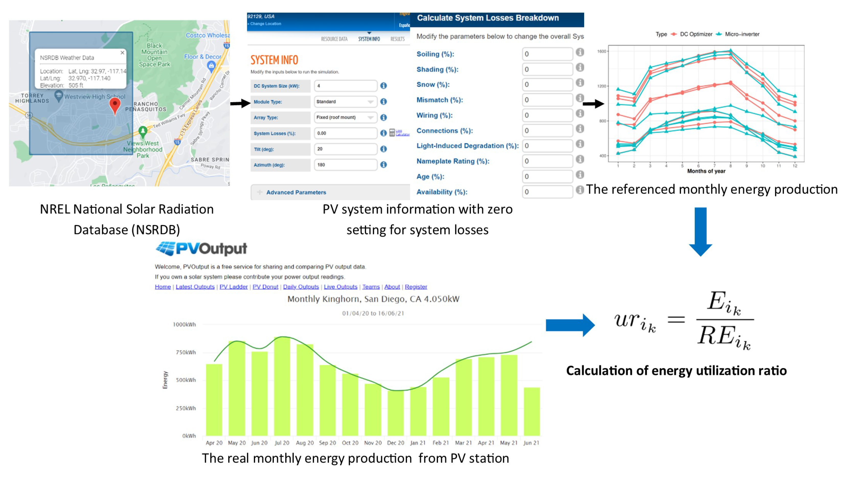
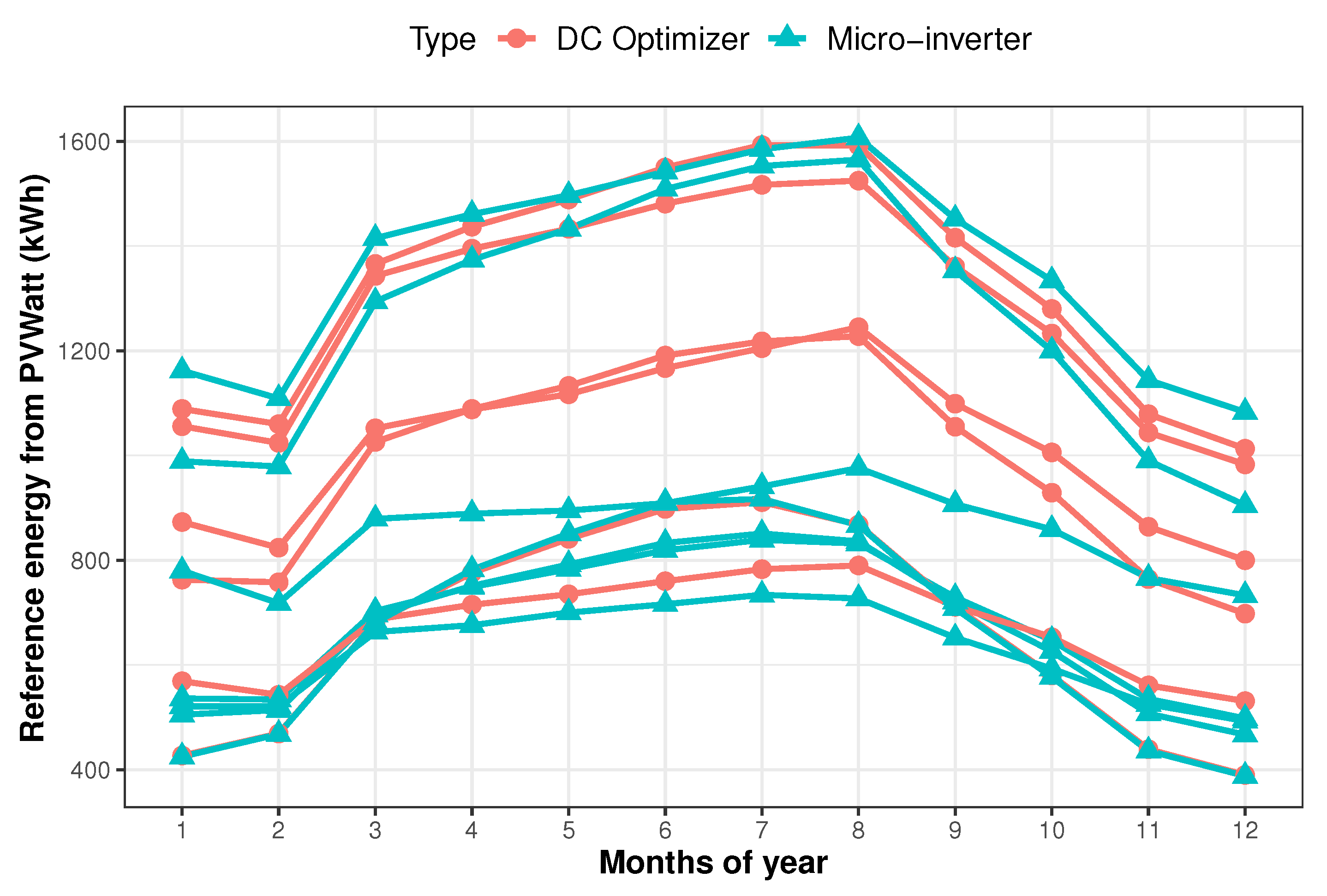
The monthly energy output (measured after the inverter), $E_i$, has the same definition as the final system yield in Standard IEC 61724. The index k represents the kth month of the year. In this study, we generated the referenced energy production $R{E}_{i_k}$ of the ith station in Table 1 based on the PVWatt tool [26]. This is a popular software tool for estimating the PV energy production and is recommended by the national laboratory of the U.S. Department of Energy (NREL). $R{E}_{i_k}$ was estimated in the case of the ideal condition as Definition 2. Other PV setups in PVWatt such as module type, total number of panels, inverter type, total number of inverters, orientation, and tilt degrees were the same as the real PV station. The flowchart of estimating the referenced monthly energy production based on the PVWatt tool and calculating the energy utilization ratio is given in Figure 2. The result of the referenced energy production $R{E}_{i_k}$ of the rooftop PV stations in Table 1 is shown in Figure 3.

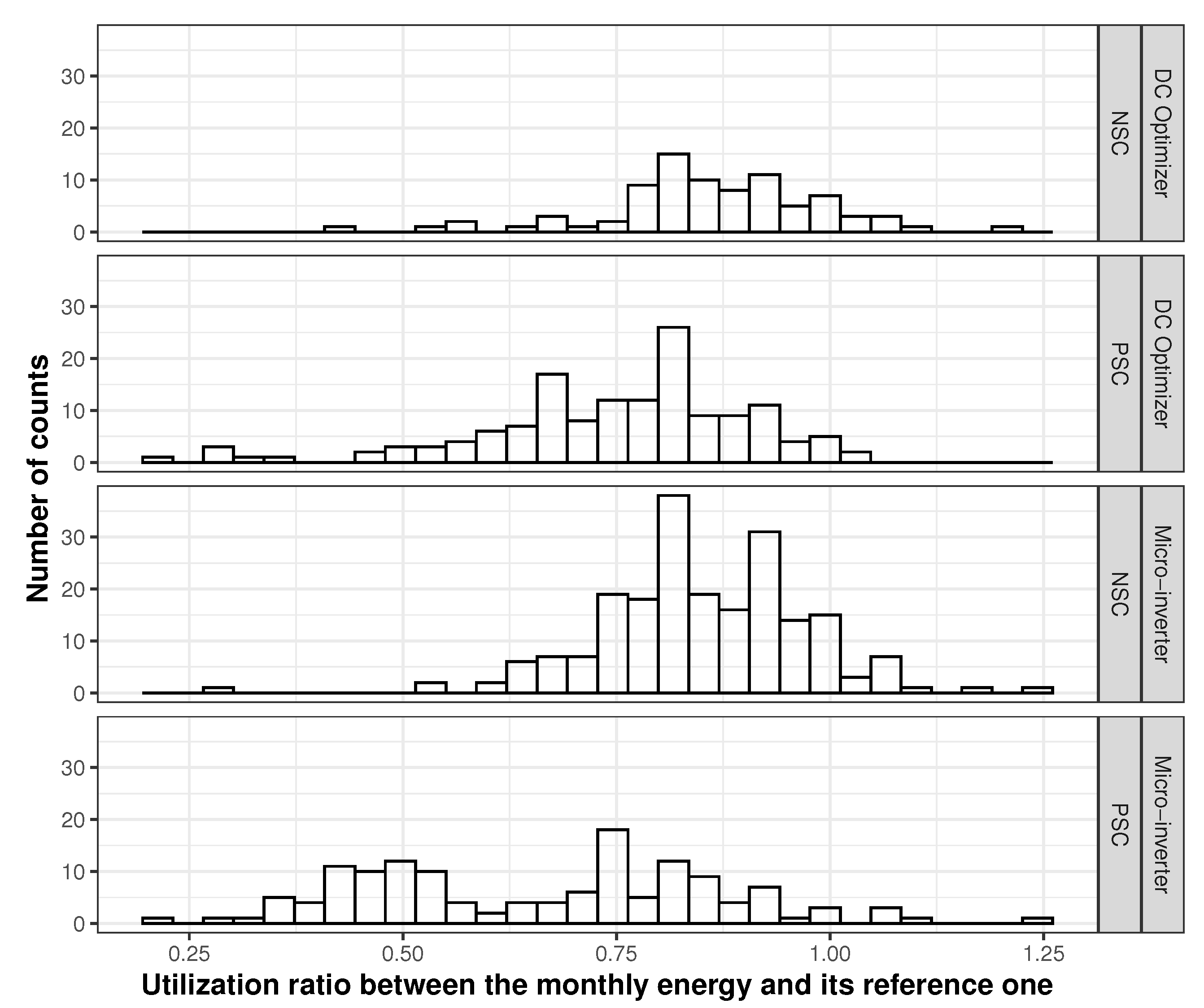
Figure 4 plots the distribution of the utilization ratio $u{r}_i$ of the ith PV station in each PV configuration according to NSC and PSC. In Section 2.2, we formulate the common utilization ratio of both PV configurations based on the mixed-effects model and evaluate its utilization ratio under the effect of PSC.

Table 2. PV stations located in Kinghorn, San Diego, CA, USA (postcode: 92129) used in study of the annual energy yield. The chosen stations share the same postcode (within 4 km). Thus, they are assumed to suffer similar weather condition. PSC decrease temporarily the amount of radiation reaching the solar panels.

Name	Installed Power (kW)	MPPT Method	PV Array		Inverter Configuration		Orientation	PSC	Tilt Degrees
			Rated Power (W)	Total Panel	Rated Power (W)	Number of Inverters
Kinghorn	4.05	DC optimizer	270	15	3800	1	South	Yes	23
Barrymore plant	4.48	DC optimizer	280	16	6000	1	South west	No	1
IIIudium Q-36	6.36	DC optimizer	335	19	7600	1	South west	Yes	37
Across the park	4.23	Microinverter	235	12	190	12	South	No	15
Koobzilla	3.84	Microinverter	240	16	215	16	South	No	22
Solar Bob	5.13	Microinverter	270	19	250	19	South	No	33
JCG’s Almazon System	4.25	Microinverter	250	17	215	17	South	Yes	11
ZzPV	8.16	Microinverter	285	28	250	28	South	Yes	24

shows the list of the rooftop PV stations used in the second study. We chose the annual energy yield as the variable to estimate the annual degradation rate of PV stations. The annual energy yield was calculated as Equation (2),

$$y=\frac{{\sum }_{j=1}^Y{E}_{da{y}_j}}{Y.P_{pv}}\left(\mathrm{kWh}/\mathrm{kW}\right)$$

(2)

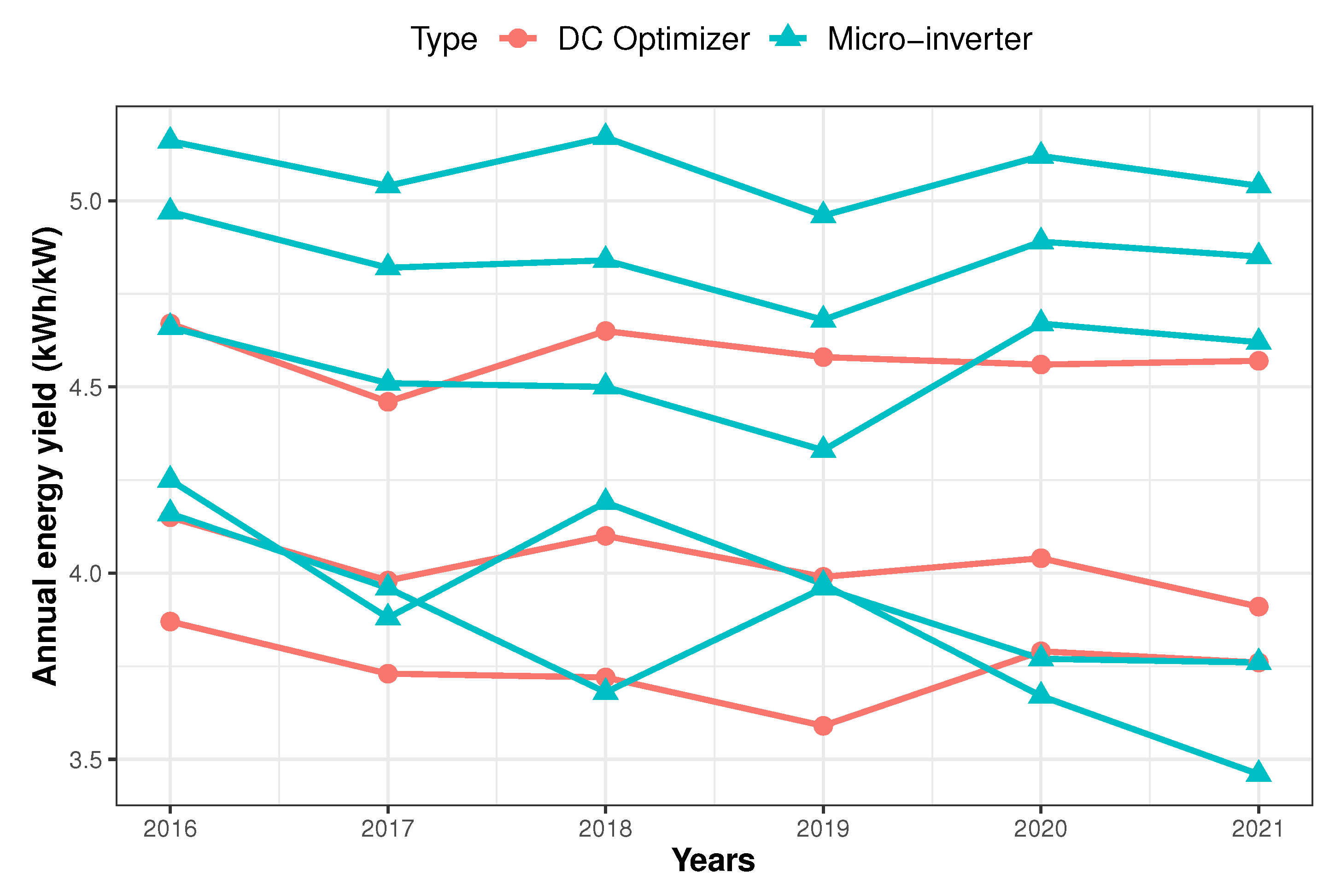
where $P_{pv}$ is the rated power of the PV system, Y is the total number of recorded days of the yth year, and $E_{da{y}_j}$ is the total generated energy from the PV system on the jth day. Figure 5 shows the resulting yearly yields for the PV stations with two different configurations. In Section 2.2, we formulate these yields as a linear decline model using a mixed-effects model to estimate the degradation rate and evaluate the effect of PSC on the degradation rate.

2.2. The Applied Mixed-Effects Model

The mixed-effects model (MEM) is increasingly recognized as an effective method in power engineering instead of the test-of-variation (ANOVA) method in power engineering [21,22,27,28] to compare many grouped objects whose datasets are time series and grouped [29]. In our study, we proposed two models based on an MEM: an average model to find the effect of PSC on the energy utilization ratio and a linear decline model to evaluate the effect of PSC on the annual degradation rate. In our study, the PV stations were grouped into NSC and PSC groups. In the regression aspect, each MEM combined fixed effects and random effects linearly. While the former reflect the value of the observed variable representing each group, the latter reflect the random variability of this observed variable among many groups. By determining the fixed-effects terms for grouped objects, any differences among groups could be determined easily. The mixed-effects model’s further theories and computational methods are referenced in [28,29].

2.2.1. Average Model Based on MEM: Finding the PSC’s Effect on Energy Utilization Ratio

In this model, the utilization ratio $u{r}_{is}$ of the ith PV station and the group s was a linear combination of its average utilization ratio ${UR}_{is}$ and the residuals or errors between the $u{r}_{is}$ value and ${UR}_{is}$. The index $s=0$ indicates the ith PV station belongs to the NSC group, and $s=1$ indicates the ith PV station belongs to the PSC group. The formula is represented as in Equation (3):

$$u{r}_{is}={UR}_{is}+r_{is}$$

(3)

The residual $r_{is}$ was assumed to follow a normal distribution with zero mean and variance ${\sigma }_r^2$, $r_{is}\sim \mathcal{N}(0,{\sigma }_r^2)$. Since we explored whether there was any difference in the utilization ratio of PV stations between the NSC and PSC groups, we formulated $U{R}_{is}$ as another linear combination shown in Equation (4):

$${UR}_{is}={UR}_0+s\left({UR}_{0s}\right)+{\lambda }_s$$

(4)

where ${UR}_0$ is the common utilization ratio value for the NSC PV stations in Table 1. $U{R}_{0s}$ is the difference of utilization ratio for the PSC group ($s=1$). The residual ${\lambda }_s$ was assumed to follow a normal distribution with zero mean and variance ${\sigma }_{\lambda }^2$, $u_s\sim \mathcal{N}(0,{\sigma }_{\lambda }^2)$.

By substituting Equation (4) to Equation (3), the formula in Equation (3) was written as Equation (5) as follows:

$$\begin{array}{cc}\hfill u{r}_{is}& =[{UR}_0+s\left({UR}_{0s}\right)+{\lambda }_s]+r_{is}\hfill \\ \hfill & =[{UR}_0+s\left({UR}_{0s}\right)]+({\lambda }_s+r_{is})\hfill \end{array}$$

(5)

The fixed effect in Equation (5) is $[{UR}_0+s\left({UR}_{0s}\right)]$, which reflects the average utilization ratio of a particular PV system considering the effect of PSC. In addition, if there occurs any significant difference in the average utilization ratio between the two groups, then ${UR}_{0s}$ determines how large the difference is. In general, the result comparison of the average model based on an MEM is followed by a hypothesis test as below:

• The null hypothesis ($H_0$): There is no significant difference in the average utilization ratio between the PSC and NSC groups. This means MLPE have improved the ability of energy harvesting in the case of PSC. If the p-value (the probability assuming that the null hypothesis is correct) is larger than $0.05$, then $H_0$ can be assumed;
• The alternative hypothesis ($H_1$): there is a significant difference in the average utilization ratio between the PSC and NSC groups ($p<0.05$).

The scatter quantile–quantile (Q-Q) plot was used to test the random-effect assumption and verify the robustness of the model based on an MEM [30,31,32]. This scatter plot was created by drawing two sets of quantiles against one another. If both came from the same distribution, then we obtained the points forming a roughly straight line. The average utilization ratio comparisons of PV groups are shown in Section 3.1.

2.2.2. Linear Decline Model Based on MEM: Finding the PSC’s Effect on the Annual Degradation Rate

This model assumed that the degradation trend of the annual yield $y_i$ (kWh/kW) in Figure 5 was linear. This assumption was adequate for a short period, as in our previous study [27]. Hence, we formulated the annual energy yield as Equation (6):

$$y_i={\alpha }_i+{\beta }_{i}t+e_i$$

(6)

where $y_i$ is the observed energy yield for individual PV stations $i=1,2,\dots ,8$, collected repeatedly every year from 2016 to 2021 and noted by the index of the year $t=0,1,\dots ,5$. The ${\alpha }_i$’s and ${\beta }_i$’s correspond to the baseline yield and annual degradation rate of the ith PV station, respectively. Actually, the baseline yield was the initial energy yield that we obtained in 2016, and $e_i$ was the error (or residual) between the real value and the calculated value from the model of the ith PV station. The error $e_i$ was assumed to follow a normal distribution with zero mean and variance ${\sigma }_e^2$, $e_i\sim \mathcal{N}(0,{\sigma }_e^2)$.

Since we intended to investigate whether there existed any significant difference in the coefficients of the linear decline model under the effect of PSC, the parameters ${\alpha }_i$ and ${\beta }_i$ were rewritten as in Equation (7) to reflect the impact of PSC:

$$\begin{array}{cc}\hfill {\alpha }_i& =A_0+A_1{S}_i+u\hfill \\ \hfill {\beta }_i& =B_0+B_1{S}_i+v\hfill \end{array}$$

(7)

where $A_0$ and $B_0$ are the baseline yield and annual degradation rate of all PV stations under NSC ($S=0$), and $A_1$ and $B_1$ represent the amount of baseline yield and annual degradation rate caused by the effect of PSC ($S=1$). The error terms u and v were inferred to follow a normal distribution with their respective variances $u\sim \mathcal{N}(0,{\sigma }_u^2)$ and $v\sim \mathcal{N}(0,{\sigma }_v^2)$.

By substituting Equation (7) to Equation (6), the formula in Equation (6) was written as Equation (8) below:

$$\begin{array}{cc}\hfill y_i& =(A_0+A_1{S}_i+u)+(B_0+B_1{S}_i+v)t+e_i\hfill \\ \hfill & =[(A_0+A_1{S}_i)+(B_0+B_1{S}_i)t]+(u+vt)+e_i\hfill \end{array}$$

(8)

The fixed-effects part $[(A_0+A_1{S}_i)+(B_0+B_1{S}_i)t]$ represents the decreasing trend of the annual energy yield for all PV groups in Table 2, taking into account the influence of PSC. In addition, if there occurs any significant difference between the two groups, then $A_1$ and $B_1$ identify how significant the difference is. The resulting analysis of the linear decline model based on an MEM is shown in Section 3.2. In general, the result comparison of the linear decline model based on an MEM is followed by a hypothesis test as below:

• The null hypothesis ($H_0$): There is no significant difference in the trend of the annual energy yield between the PSC and NSC groups. If the p-value (the probability assuming that the null hypothesis is true) is larger than $0.05$, then $H_0$ can be assumed;
• The alternative hypothesis ($H_1$): there is a significant difference in the trend of the annual energy yield between the PSC and NSC groups ($p<0.05$).

3. Analysis Results

The proposed models in our study were programmed using R version 3.4.0 [33] and the nlme package [34]. The random process used the same number of generators to guarantee reproducibility [30,31,32].

3.1. The PSC’s Effect on the Energy Utilization Ratio

Table 3. The fixed-effects results of the average model based on the MEM in Equation (5).

Fixed Effects	Meaning	Value (%)	95% CI	p Value	Mean Square Error (MSE)
$U{R}_0$	The common utilization ratio of PV stations in NSC group	$85.8\%$	($78.1\%$ to $93.5\%$)	<0.0001	$245.6$
$U{R}_{01}$	The difference of utilization ratio between PSC and NSC groups	$-14.7\%$	($-27.3\%$ to $-2.0\%$)	$0.026$

shows the resulting parameters of the fixed-effects part from an average model based on an MEM. From this table, we conclude about the influence of PSC on the rooftop PV systems using MLPE as follows:

• The common utilization ratio of PV stations in the NSC group in Table 1 was about $85.8\%$, and its $95\%$ confidence interval (CI) was from $78.1\%$ to $93.5\%$;
• For PV stations in the PSC group, there was a significant reduction in the utilization ratio, regardless of the types of MLPE (DC optimizer and microinverter), which was about $-14.7\%$ and its $95\%$ (CI) was from $-27.3\%$ to $-2.0\%$. In addition, the p-value of $U{R}_{01}$ was $0.026$ (<$0.05$), which identified the resulting value as statistically significant.

Unlike our expectation, the above result indicated that the rooftop PV stations obtained a significant reduction of about $-14.7\%$ in their utilization ratio under the impact of PCS. This meant that the existing SolarEdge DC optimizer and Enphase microinverter actually did not effectively improve the energy harvesting of the PV systems in real working conditions with the impact of PSC.

The random-effects values and R-squared of the average model based on an MEM are shown in

Table 4. The random-effects results of the average model based on the MEM in Equation (5).

Random Effects	Source of Variance	Variance	R-Squared
${\sigma }_{\lambda }^2$	Variance among PV stations in two groups	$102.5$	$\frac{{\sigma }_{\lambda }^2}{{\sigma }_{\lambda }^2+{\sigma }_r^2}=40\%$
${\sigma }_r^2$	Residuals (errors) from each PV station	$154.2$

. The R-squared represents the proportion of variance in the utilization ratio of PV stations in Table 1, which the model can explain. From the R-squared result, we interpreted that our proposed model could explain up to $40\%$ of the total variation of the utilization ratio.

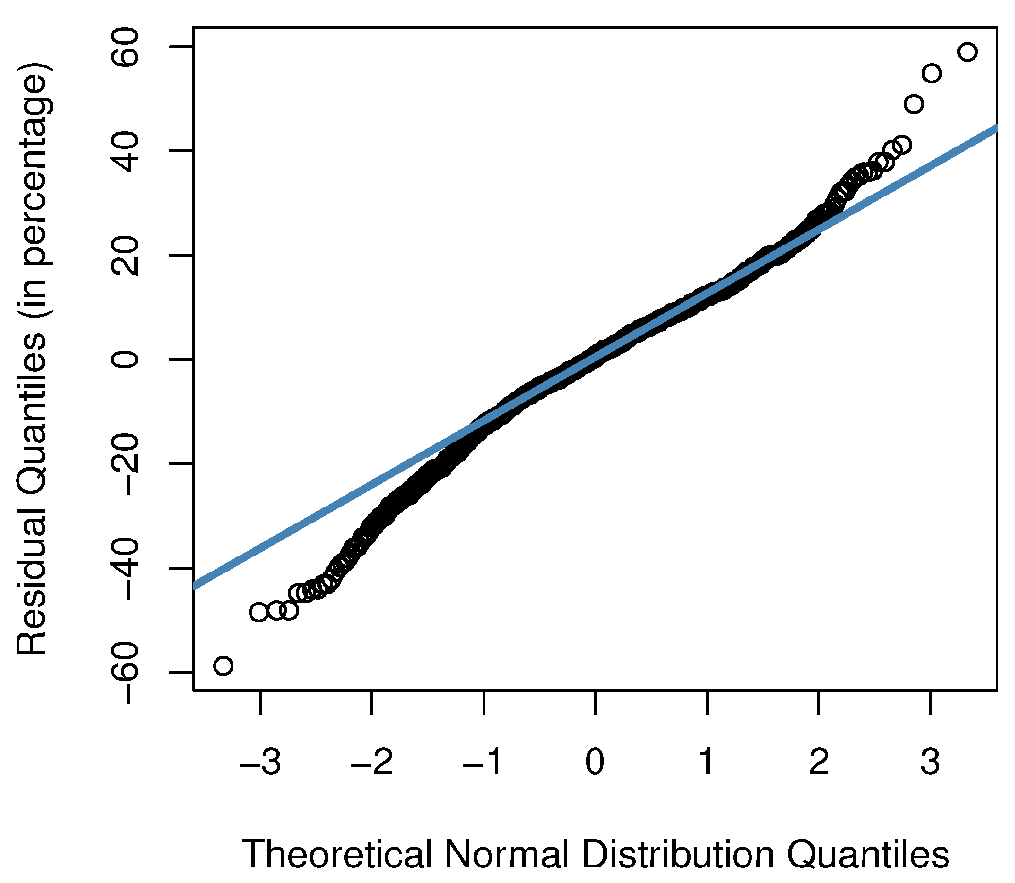
To show the advantage of our proposed average model, we conducted an ANOVA test to investigate whether there was any significant difference in the utilization ratio between the PSC and NSC groups. Although the result from the ANOVA in

Table 5. The analysis result from the ANOVA test.

ANOVA Test	Source of Variation	Degrees of Freedom	Sum of Square	Mean Square	F-Test	p Value
Effect of PSC	Between two PV groups	1	30970	30970	125.8	<0.0001
	Within a PV group	575	141581	246.2

confirmed a significant difference in the energy utilization ratio, its limitation was that the ANOVA did not provide how much this difference was. Finally, the Q-Q plot in Figure 6 depicts that all the points are located approximately along the reference line. Therefore, we can assume the normality of the residuals and also the robustness of the proposed average model based on an MEM.

3.2. The PSC’s Effect on the Annual Degradation Rate

Table 6. The fixed-effects results of the linear decline model based on the MEM in Equation (8).

Parameter	Meaning	Value (kWh/kW)	95% CI (kWh/kW)	p Value
$A_0$	Baseline energy yield of NSC group	$4.59$	($4.14$ to $5.04$)	<0.0001
$B_0$	Degradation rate of NSC group	$-0.05$	($-0.097$ to $-0.003$)	$0.037$
$A_1$	Difference in baseline energy yield between PSC and NSC groups	$-0.35$	($-1.12$ to $0.42$)	$\mathbf{0}.\mathbf{31}$
$B_1$	Difference in degradation rate between PSC and NSC groups	$0.029$	($-0.037$ to ($0.096$)	$\mathbf{0}.\mathbf{38}$

shows the resulting parameters of the fixed-effects term of the linear decline model and their corresponding $95\%$ CI. From these results, the linear decline model that represents the annual energy yield of the PV stations belonging to the NSC group ($S=0$) in Table 2 was:

$$y\left(t\right)=A_0+B_{0}t=4.59-0.05t$$

(9)

The linear decline model for the PV stations belonged to the PSC group ($S=1$) was:

$$\begin{array}{cc}\hfill t_i& =(A_0+A_1{S}_i)+(B_0+B_1{S}_i)t\hfill \\ \hfill & =(4.59+(-0.35\left)1\right)+(-0.05+(0.029\left)1\right)t\hfill \\ \hfill & =4.24-0.021t\hfill \end{array}$$

(10)

However, Table 6 confirmed there was no significant difference between the linear decline models in Equations (9) and (10) since the obtained p values of $A_1$ and $B_1$ were $0.31$ and $0.38$, which are larger than $0.05$. Therefore, the null hypothesis ($H_0$) in the Section 2.2.2 could be assumed. In addition, the $95\%$ CI ranges of $A_1$ and $B_1$ in Table 6 also crossed the zero value. Therefore, the result implied that there was no evidence of the PSC’s effect on reducing the degradation rate of the rooftop PV stations using MLPE in Table 2.

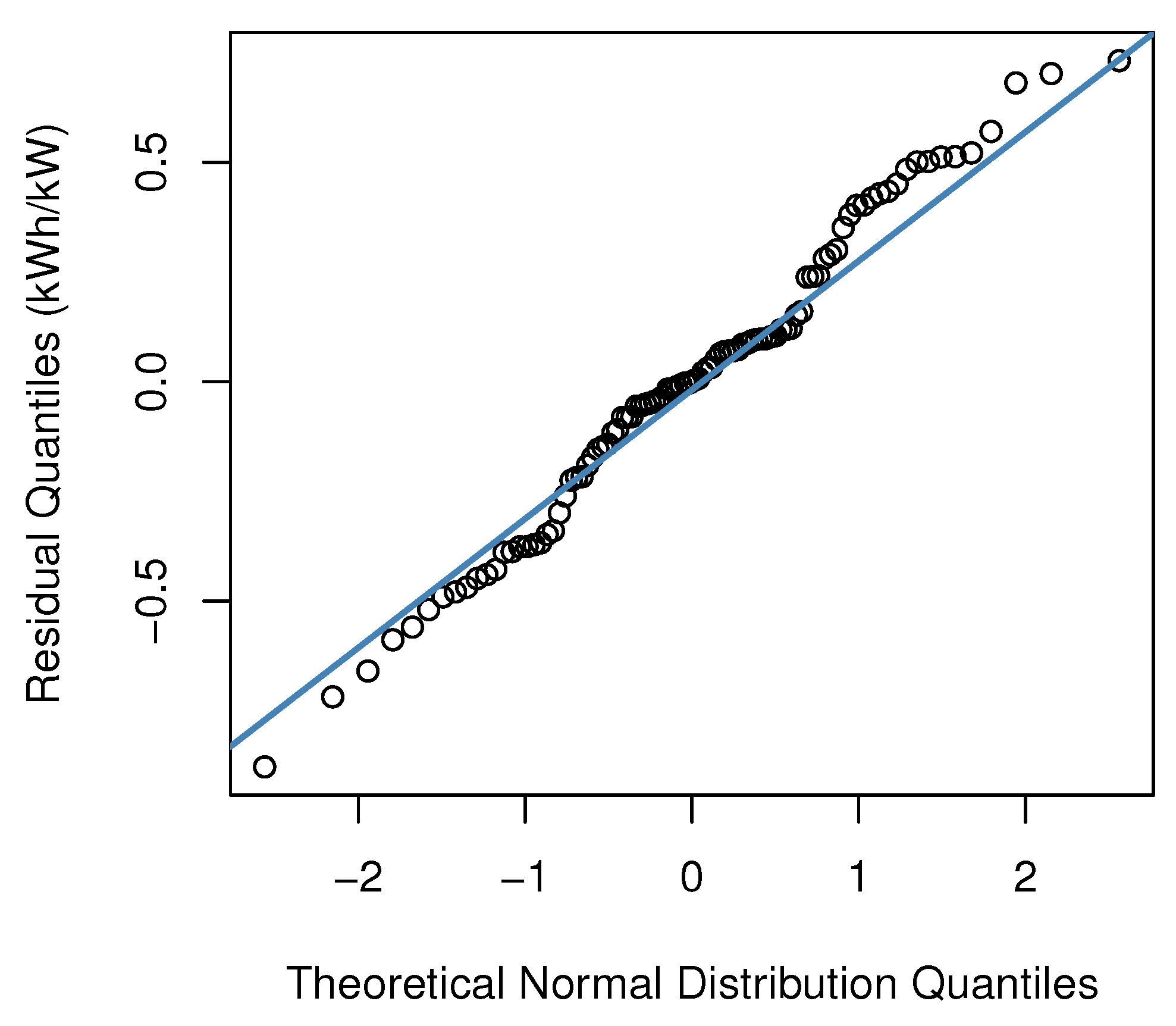
The R-squared value in

Table 7. The random-effects results of the linear decline model based on the MEM in Equation (8).

Parameter	Source of Variance	Variance	R-Squared
${\sigma }_u^2$	Baseline energy yield	$0.44$	$\frac{{\sigma }_u^2+{\sigma }_v^2}{{\sigma }_u^2+{\sigma }_v^2+{\sigma }_e^2}=80\%$
${\sigma }_v^2$	Degradation rate	$0.037$
${\sigma }_e^2$	Residuals	$0.119$

indicates the robustness of the proposed linear decline model since it can explain about $80\%$ of the variation of annual yield from PV stations. Finally, Figure 7 shows a Q-Q plot of the residuals from the linear decline model. Since all the points are located approximately along the reference line, we can assume the normality of residuals and the robustness of model.

4. Discussion

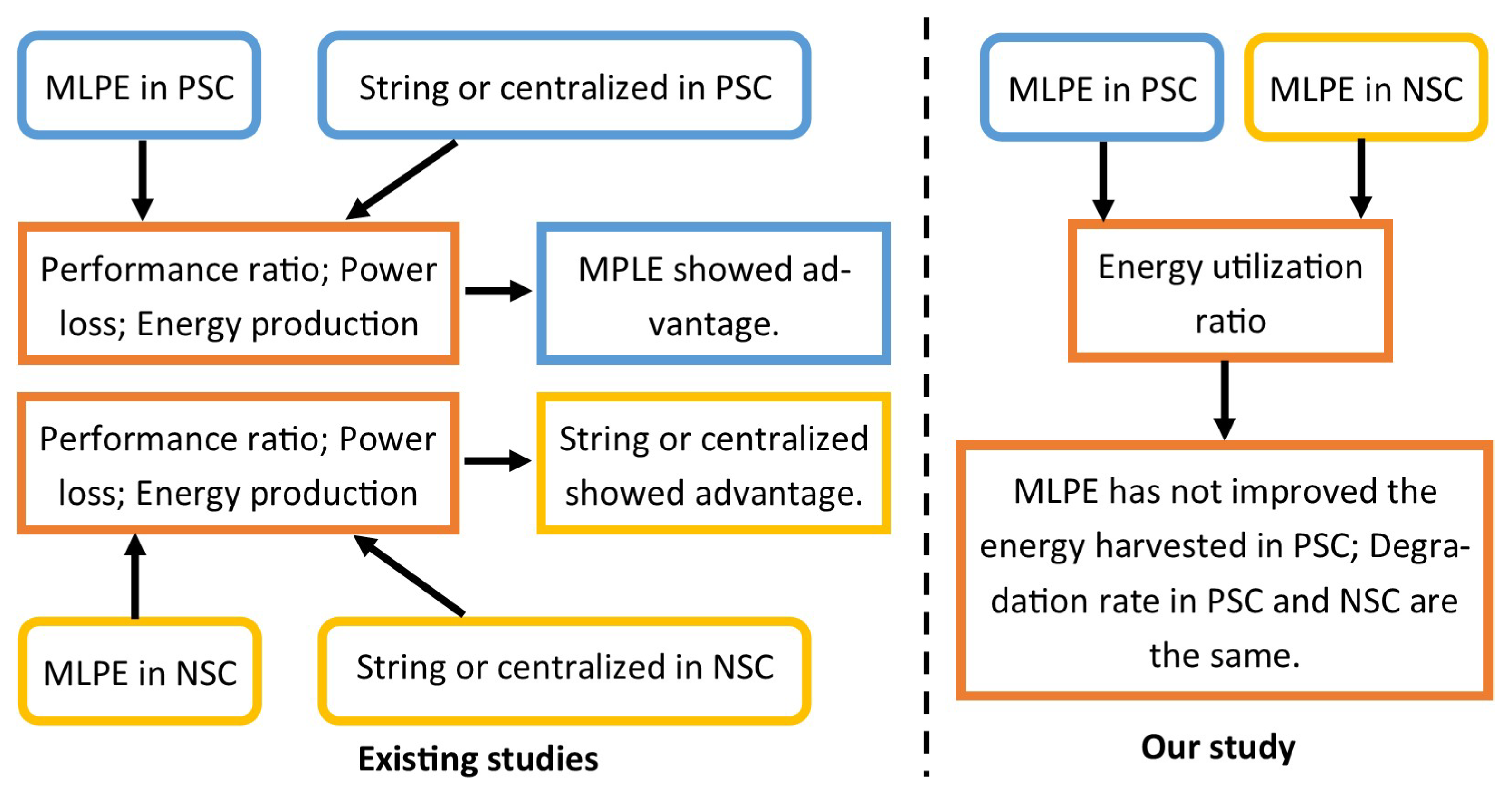
Our results are consistent with existing studies in the literature review about the advantage of rooftop PV systems using MLPE to eliminate the effect of PSC on the annual degradation rate. However, more studies are required to verify the ability of improving the energy harvested from PV systems under PSC. While other studies in the literature [12,13,14,15,16,17,18,19] have shown the advantage of using MLPE (microinverter or DC optimizer) over the string or centralized inverter under partial shading conditions and in nonshading conditions, the energy performance of a string or centralized inverter is shown to outperform MLPE (especially when the string or centralized inverter is integrated with MPPT (maximum power point tracking)), our study revealed for the first time, (while, to the extent of our knowledge, the past literature did not), that MLPE did not effectively improve the energy harvested from PVs under PSC compared with that in NSC. While MLPE were designed to recover the power loss from panel mismatch, the string or centralized inverter was not designed to recover the power loss from panel mismatch, so the comparison between PV systems using MPLE and PV systems using a string or centralized inverter under PSC seems unfair. Finally, Figure 8 summarizes the difference between our study and other existing studies [12,13,14,15,16,17,18,19].

Our finding could then be used by homeowners for their decision-making, as a recommendation to select the gained energy production under PSC or the cost of a rooftop PV system using MLPE for their investment. Our finding also suggests that in the area where partial shading rarely happens, the rooftop PV system using a string or centralized inverter configuration is a more appropriate option than MLPE. Finally, our findings also provide helpful information to include in other studies, such as forecasting the energy production or calculating the levelized cost of electricity (LCOE) [35,36,37,38] of such types of PV systems.

5. Conclusions

This study verified the advantage of using MLPE for rooftop PV system to reduce the effect of PSC using a real-world PVs dataset at Kinghorn city, San Diego, CA. The finding showed that the energy utilization ratio of PV systems with MLPE had a significant reduction of about $14.7\%$ (with $95\%$ confidence interval: $-27.3\%$ to $-2.0\%$) under PSC, compared to that under nonshading conditions (NSC). In addition, the annual degradation rate of the PV systems was about $-50$ (Wh/kW) and the PSC did not affect to this rate. Our work provided more information about the MLPE’s ability to reduce the effect of PSC and help the homeowner make a better decision for their PV system installation.

Future work will extend our proposed mixed-effects model to find the energy yield of the PV system using a power optimization device at the module level that can be generalized for many regions. Another work will take into account the rooftop PV systems using a string or central inverter integrated MPPT function to compare the energy production of MPPT techniques on different levels under the effect of partial shading.

References

1. Francisco Contero, J.; Gomes, J.; Gustafsson, M.; Karlsson, B.O. The impact of shading in the performance of three different solar PV systems. In Proceedings of the 11th ISES Eurosun 2016 Conference, Palma, Spain, 11–14 October 2017; pp. 1168–1179. [Google Scholar] [CrossRef] [Green Version]
2. Alves, T.; Torres, J.P.N.; Marques Lameirinhas, R.A.; Fernandes, C.A.F. Different Techniques to Mitigate Partial Shading in Photovoltaic Panels. Energies 2021, 14, 3863. [Google Scholar] [CrossRef]
3. Toufik, S.; Ridha, K.; Abdelouahab, Z. An experimental validation of the effect of partial shade on the I-V characteristic of PV panel. Int. J. Adv. Manuf. Technol. 2018, 96, 4165–4172. [Google Scholar] [CrossRef]
4. Zheng, H.; Li, S.; Proano, J. PV energy extraction characteristic study under shading conditions for different converter configurations. In Proceedings of the 2012 IEEE Power and Energy Society General Meeting, San Diego, CA, USA, 22–26 July 2012; pp. 1–8. [Google Scholar]
5. Gallardo-Saavedra, S.; Karlsson, B. Simulation, validation and analysis of shading effects on a PV system. Sol. Energy 2018, 170, 828–839. [Google Scholar] [CrossRef]
6. Galtieri, J.; Krein, P.T. Energy improvements from subpanel DC-DC converters in PV arrays with distributed mismatch. In Proceedings of the 2016 IEEE 43rd Photovoltaic Specialists Conference (PVSC), Portland, OR, USA, 5–10 June 2016; pp. 3213–3218. [Google Scholar]
7. Sarwar, S.; Javed, M.Y.; Jaffery, M.H.; Ashraf, M.S.; Naveed, M.T.; Hafeez, M.A. Modular Level Power Electronics (MLPE) Based Distributed PV System for Partial Shaded Conditions. Energies 2022, 15, 4797. [Google Scholar] [CrossRef]
8. Nafeh, A.E.S.A. Novel Maximum-Power-Point Tracking Algorithm For Grid-Connected Photovoltaic System. Int. J. Green Energy 2010, 7, 600–614. [Google Scholar] [CrossRef]
9. Birane, M.; Larbes, C.; Cheknane, A. Comparative study and performance evaluation of central and distributed topologies of photovoltaic system. Int. J. Hydrogen Energy 2017, 42, 8703–8711. [Google Scholar] [CrossRef]
10. SolarEdge Power Optimizer. Available online: https://www.solaredge.com/products/power-optimizer/ (accessed on 20 November 2022).
11. Enphase Microinverter. Available online: https://enphase.com/en-us/products-and-services/microinverters (accessed on 20 November 2022).
12. Deline, C.; Meydbray, J.; Donovan, M. Photovoltaic Shading Testbed for Module-Level Power Electronics: 2016 Performance Data Update; Technical Report Contract No. DE-AC36-08GO28308; NREL National Renewable Energy Laboratory: Golden, CO, USA, 2016.
13. Deline, C.; Marion, B.; Granata, J.; Gonzalez, S. A Performance and Economic Analysis of Distributed Power Electronics in Photovoltaic Systems; Technical Report Contract No. DE-AC36-08GO28308; NREL National Renewable Energy Laboratory: Golden, CO, USA, 2011. [Google Scholar]
14. Sinapis, K.; Litjens, G.; van den Donker, M.; Folkerts, W.; van Sark, W. Outdoor characterization and comparison of string and MLPE under clear and partially shaded conditions. Energy Sci. Eng. 2015, 3, 510–519. [Google Scholar] [CrossRef]
15. Tsafarakis, O.; Sinapis, K.; van Sark, W.G.J.H.M. A Time-Series Data Analysis Methodology for Effective Monitoring of Partially Shaded Photovoltaic Systems. Energies 2019, 12, 1722. [Google Scholar] [CrossRef] [Green Version]
16. Hernández-Callejo, L.; Gallardo-Saavedra, S.; Diez-Cercadillo, A.; Gómez, V.A. Analysis of the influence of DC optimizers on photovoltaic production. Rev. Fac. Ingeniería Univ. Antioq. 2020, 94, 43–55. [Google Scholar] [CrossRef]
17. Mehedi, I.; Salam, Z.; Ramli, M.; Chin, V.; Bassi, H.; Rawa, M.; Abdullah, M. Critical evaluation and review of partial shading mitigation methods for grid-connected PV system using hardware solutions: The module-level and array-level approaches. Renew. Sustain. Energy Rev. 2021, 146, 111138. [Google Scholar] [CrossRef]
18. Wang, Q.; Le, L.; Li, D.; Ai, X.; Fang, J.; Yao, W.; Wen, J. Modeling and Energy Generation Evaluations of Large-Scale Photovoltaic Plants Equipped With Panel-Level DC Optimizers. Front. Energy Res. 2022, 10, 30. [Google Scholar] [CrossRef]
19. Hanson, A.J.; Deline, C.A.; MacAlpine, S.M.; Stauth, J.T.; Sullivan, C.R. Partial-Shading Assessment of Photovoltaic Installations via Module-Level Monitoring. IEEE J. Photovolt. 2014, 4, 1618–1624. [Google Scholar] [CrossRef]
20. IEC TS 61724-3:2016; Photovoltaic System Performance-Part 3: Energy Evaluation Method. Available online: https://webstore.iec.ch/publication/25466 (accessed on 20 November 2022).
21. Roach, C. Estimating electricity impact profiles for building characteristics using smart meter data and mixed models. Energy Build. 2020, 211, 109686. [Google Scholar] [CrossRef]
22. Simões, P.F.M.; Souza, R.C.; Calili, R.F.; Pessanha, J.F.M. Analysis and short-term predictions of non-technical loss of electric power based on mixed effects models. Socio-Econ. Plan. Sci. 2020, 71, 100804. [Google Scholar] [CrossRef]
23. Haynes, W. Student’s t-Test. In Encyclopedia of Systems Biology; Dubitzky, W., Wolkenhauer, O., Cho, K.H., Yokota, H., Eds.; Springer: New York, NY, USA, 2013; pp. 2023–2025. [Google Scholar] [CrossRef]
24. ANOVA Method For Comparison Models. Available online: https://www.rdocumentation.org/packages/ltm/versions/1.1-1/topics/anova (accessed on 20 November 2022).
25. PVOutput Dataset. Available online: https://pvoutput.org/ (accessed on 20 November 2022).
26. PVWatts Calculator. Available online: https://pvwatts.nrel.gov/pvwatts.php (accessed on 20 November 2022).
27. Le, N.T.; Benjapolakul, W. Comparative Electrical Energy Yield Performance of Micro-Inverter PV Systems Using a Machine Learning Approach Based on a Mixed-Effect Model of Real Datasets. IEEE Access 2019, 7, 175126–175134. [Google Scholar] [CrossRef]
28. Le, N.T.; Asdornwised, W.; Chaitusaney, S.; Benjapolakul, W. Application of The Mixed Effects Model for Analyzing Photovoltaic Datasets and Interpreting Into Meaningful Insights. IET Gener. Transm. Distrib. 2021, 15, 2101–2111. [Google Scholar] [CrossRef]
29. Pinheiro, J.C.; Bates, D.M. Mixed-Effects Models in S and S-PLUS. In Statistics and Computing; Springer: New York, NY, USA, 2000. [Google Scholar] [CrossRef]
30. Garcia, T.P.; Ma, Y.; Marder, K.; Wang, Y. Robust mixed effects model for clustered failure time data: Application to Huntington’s disease event measures. Ann. Appl. Stat. 2017, 11, 1085–1116. [Google Scholar] [CrossRef] [PubMed]
31. Schielzeth, H.; Dingemanse, N.J.; Nakagawa, S.; Westneat, D.F.; Allegue, H.; Teplitsky, C.; Réale, D.; Dochtermann, N.A.; Garamszegi, L.Z.; Araya-Ajoy, Y.G. Robustness of linear mixed-effects models to violations of distributional assumptions. Methods Ecol. Evol. 2020, 11, 1141–1152. [Google Scholar] [CrossRef]
32. Warrington, N.M.; Tilling, K.; Howe, L.D.; Paternoster, L.; Pennell, C.E.; Wu, Y.Y.; Briollais, L. Robustness of the linear mixed effects model to error distribution assumptions and the consequences for genome-wide association studies. Stat. Appl. Genet. Mol. Biol. 2014, 13, 567–587. [Google Scholar] [CrossRef] [Green Version]
33. The R-Project for Statistical Computing. Available online: https://cran.r-project.org/bin/windows/base/ (accessed on 20 November 2022).
34. Pinheiro, J.; Bates, D.; DebRoy, S.; Sarkar, D.; R Core Team. Nlme: Linear and Nonlinear Mixed Effects Models; CRAN: Chicago, IL, USA, 2018. [Google Scholar]
35. Simple Levelized Cost of Energy (LCOE) Calculator Documentation. Available online: https://www.nrel.gov/analysis/tech-lcoe-documentation.html (accessed on 20 November 2022).
36. Lai, C.S.; McCulloch, M.D. Levelized cost of electricity for solar photovoltaic and electrical energy storage. Appl. Energy 2017, 190, 191–203. [Google Scholar] [CrossRef]
37. Mundada, A.S.; Shah, K.K.; Pearce, J. Levelized cost of electricity for solar photovoltaic, battery and cogen hybrid systems. Renew. Sustain. Energy Rev. 2016, 57, 692–703. [Google Scholar] [CrossRef] [Green Version]
38. Kang, M.H.; Rohatgi, A. Quantitative analysis of the levelized cost of electricity of commercial scale photovoltaics systems in the US. Sol. Energy Mater. Sol. Cells 2016, 154, 71–77. [Google Scholar] [CrossRef]
Figure 1. The schematics of DC optimizer configuration (left) and microinverter configuration (right) for rooftop PV system.
Energies 16 00970 g001
Figure 2. The flowchart of estimating the referenced monthly energy production based on the PVWatt tool and calculating the energy utilization ratio.
Energies 16 00970 g002
Figure 3. The referenced monthly energy of the DC optimizer and microinverter rooftop PV systems in Table 1 generated from the PVWatts tool [26].
Energies 16 00970 g003
Figure 4. The distribution plots of the utilization ratio ( u r ) of the DC optimizer and microinverter PV systems in Table 1 under NSC and PSC. The u r can be larger than 1 since the actual number of sun hours for some months are higher than the estimated ones.
Energies 16 00970 g004
Figure 5. The plot of the annual energy yield of PV stations in Table 2 from 2016 to 2021 which were used for the annual degradation rate analysis.
Energies 16 00970 g005
Figure 6. The Q-Q plot of average model. The points located approximately along the reference line (blue line) indicate that the residuals’ normality assumption is acceptable.
Energies 16 00970 g006
Figure 7. The Q-Q plot of linear decline model. The points located approximately along the reference line (blue line) indicate that the residuals’ normality assumption is acceptable.
Energies 16 00970 g007
Figure 8. The comparison between existing studies in literature and our study [12,13,14,15,16,17,18,19].
Energies 16 00970 g008