1. Introduction
Many computer vision problems focus on classifying a single object on a simple background. This task demands defining appropriate image features. Different image features are suitable for different applications. The key is to find features that emphasise between-class and suppress within-class variations. The search process usually utilises a classifier.
The classifier is a procedure that accepts a set of features and produces a class label for them. It is developed using a set of labelled examples to create a rule that assigns a label to any new example. The labelled examples are part of a training dataset that embraces the properties of different types of objects and their labels. To train the classifier, two steps are required: creating the labelled dataset and building the features. The dataset creation demands a manual description of each analysed image in a convenient for further processing format, whereas the building feature step performs using hand-crafted algorithms or automatic learning techniques.
Until 2012, computer vision researchers had believed that carefully hand-designed features were necessary to understand the nature of the analysed task. Consequently, many sophisticated algorithms were developed based on edge detection [
1], texture recognition [
2], visual image segmentation [
3], ultrasound image segmentation [
4] or local image feature matching [
5]. They were utilised in a wide variety of applications, such as robotic systems [
6] or autonomous vehicles [
7,
8,
9,
10].
To develop those applications, careful hand-engineering was required by a programmer who understood the domain of analysed images. This step demanded image processing techniques, such as image filtering, image enhancement or morphological operations. They facilitated defining appropriate features in low-dimensional space for easily separable classes. Based on the above techniques, some algorithms for more complex tasks were created, such as watershed segmentation, mean-shift clustering, GrabCut or background subtraction. Even though those algorithms advanced application development, virtually every task demanded a dedicated approach and expert knowledge.
In 2012, AlexNet [
11], constructed by Krizhevsky et al., won the ImageNet Large Scale Visual Recognition (ILSVR) Challenge 2012 competition, proving that learned features can surpass manually designed ones. AlexNet constitutes a multi-layer convolutional network trained with gradient descent. It can learn complex high-dimensional and non-linear mapping from an extensive collection of examples. This property differs from the traditional approach, where a model collects the relevant information utilising a hand-designed feature extractor. The learning capability of convolutional networks has been applied to a variety of applications, such as visual recognition [
12], multi-focus image fusion [
13], or smell analysis [
14].
The AlexNet network consists of five layers of convolution, two fully connected hidden layers, and one fully connected output layer. It utilises rectified linear unit (ReLU) activation functions, dropout, and data augmentation as regularisation techniques, and overlapping pooling to reduce the dimensions of consecutive feature maps. The other researchers used this architecture to develop more complex networks. In 2014, Simonyan et al. [
15] introduced the VGG model and won the runner-up of ILSVR 2014. The VGG model comprises modules of several identical convolutional layers in succession, followed by a pooling layer. VGG has various layer structures. For example, the VGG16 contains 16 weight levels. It connects five modules in a series to two dense layers with 4096 neurons. At the back, an output layer with 1000 classifications is attached. The VGG19, for example, has a similar structure but employs 19 weight levels.
GooggleNet/InceptionV1 to V4 [
16] is another disruptive network architecture. It employs inception modules that contain four parallel branches. The first three branches consist of convolutional layers with different dimensions to detect features of different sizes. Between them, a
1 × 1 convolutional layer is inserted to reduce model complexity. The last branch, intending to reduce resolution, consists of max pooling and a
1 × 1 convolutional layer. This architecture increases the width of the network and its adaptability to different scales and resolutions of the input images.
In 2015, ResNet, created by He et al. [
17], won the ILSVR 2015 competition. The authors focused on gradients’ disappearing and exploding in very deep networks. To mitigate those problems, they proposed residual blocks containing two
3 × 3 convolutional layers with the same number of channels. The concept of the residual blocks is based on the hypothesis that if multiple non-linear layers can approximate complicated functions, they can also approximate the residual functions. Deploying residual blocks facilitates accuracy gain from significantly increased network depth and, as a result, accomplishing better results than previous networks.
Residual and inception methods substantially impacted network architectures devoted to classification tasks. As a result, both methods were combined in Inception-ResNet [
18], PolyNet [
19] and Xception models [
20]. The most successful one, Xception [
21], uses modified depthwise separable convolution derived from Inception V3 to improve performance. It also utilises residual connections similar to ResNet that significantly expedite training steps and produce a higher accuracy rate.
Even though more sophisticated architectures have been developed, the above networks are prevalent in image classification. They were trained to distinguish 1000 classes using the ImageNet dataset [
22], which consists of 1.5 million annotated images divided into 20 000 categories. The obtained Top-1 accuracies were, respectively: VGG16 (71.3%), VGG19 (71.3%), ResNet50 (74.0%), InceptionV3 (77.9%), and Xception (79%). These methods’ high performances and accuracy make them suitable as pre-trained models in many computer vision applications.
Pre-trained models constitute a practical approach to deep learning [
23,
24]. A pre-trained model was previously trained on a large dataset, usually on a large-scale image classification task. Consequently, its spatial hierarchy of features can effectively act as a generic model for various computer vision problems. There are two ways to employ pre-train models: feature extraction and fine-tuning. Feature extraction uses the representation learned by a previously trained model to extract interesting features from a new image. It consists of adopting convolutional layers of previously trained networks, replacing dense layers with a new classifier, and training the classifier with new samples. In fine-tuning methods, apart from the new classifier, some convolutional layers are also trained to distinguish other features in the images.
The methods mentioned above have been successfully deployed in electronic component classification. Lefkaditis and Tsirigotis [
25] developed a hand-designed morphological feature extraction and classification procedure for an intelligent sorting system. They combined support vector machines and multi-layer perceptron to classify capacitors, resistors, and transistors with 92.3% accuracy. Salvador et al. [
26] used transfer learning and deep convolutional neural networks to classify discrete and surface-mount electronic components found on electronic prototypes. Their results demonstrated that InceptionV3 attained the highest accuracy of 94.64% in classifying electronic components into the following classes: resistors, capacitors, inductors, transformers, diodes, and integrated circuits.
A components’ package classification system based on a custom convolutional neural network was introduced in [
27]. The proposed model could identify the 2D pattern of electronic components using nineteen features of surface mounting devices. The experiments demonstrated a 95.8% accuracy of classification. Zhou and Zhang [
28] developed another custom network to classify electronic components into eleven categories. The custom network outperformed other pre-trained networks, such as Xception, VGG16, and VGG19, obtaining the highest accuracy in single-category and diverse component classification.
A hierarchical convolutional neural network was deployed by Hu et al. [
29]. The authors utilised the convolutional automatic coding layer to obtain the relevant feature maps. The results demonstrated that the developed network could extract depth features with a precision of 94.26%. Another approach utilised a residual network architecture to combine residual blocks with convolutional layers to classify tiny electronic components [
30]. The results showed that this combination attained 95.63% accuracy on the test set.
To solve the problem of classifying electronic components using a small dataset, Yahui et al. [
31] proposed a Siamese network. According to the authors, this solution improves the classification quality of electronic components and reduces the training cost. In [
32], Atik proposed a custom convolutional network for classifying capacitors, resistors, and diodes. To analyse its performance, she compared it with the pre-trained networks: AlexNet, ShuffleNet, SqueezeNet, and GoogleNet. The results showed that the proposed model outperformed other methods, obtaining 98.99% accuracy.
Even though some researchers have addressed the electronics component classification, the presented solutions focus on generic problems. The authors utilise datasets of electronic components created during various technological processes to classify mostly elementary objects, such as resistors, capacitors, diodes, and integrated circuits. This solution is convenient for developing a versatile system capable of classifying elementary components in various applications. Nevertheless, in many cases, a system dedicated to a specific technological process is demanded.
The technological process often employs constant lighting conditions, a static camera position and a fixed set of classified components, which can be completely different from the set dedicated to another task. Consequently, each process should possess its classification system based on an image acquisition module and a dedicated classifier trained on assigned objects. The system should be accurate and flexible, facilitating straightforward dataset creation and classifier development.
Therefore, the motivation for the present work was to develop an accurate and flexible system for electronic part classification in industrial applications. To this end, an approach was proposed for a specific technological process of radio communication device manufacturing. It was aimed at classifying ten electronics components appointed by a product engineer. The components were utilised to construct a dataset, which could be effective for neural network training. The tested network structures employed pre-trained and custom networks since both structures have proved their applicability in previous research.
The main contributions of this paper can be summarised as follows:
A method for creating a database of electronic components for a given process is proposed, and an exemplary database is developed;
Neural network structures based on a custom model and pre-trained networks are designed and deeply analysed.
The results are encouraging and show that the present method can accurately classify components in a specific technological process. Additionally, since its straightforward implementation, it can be effortlessly adapted to similar applications.
The paper is structured as follows:
Section 2 outlines the developed method. In
Section 3, the obtained results for different network structures are presented, and in
Section 4, the obtained results are discussed.
2. Materials and Methods
The research objective was to develop a method for electronic part classification in industrial applications. To this end, in the first place, a vision system was designed. It facilitated image acquisition to create a dataset of electronic components. Based on the generated dataset, a baseline model of a convolutional neural network was established. It allowed for testing the dataset’s correctness and making premises for neural network architectures.
The network architectures were designed in the subsequent step. For this purpose, a custom model and pre-trained networks were regarded. Their programming implementation was derived from the publicly available TensorFlow 2 and Keras libraries and implemented on a single graphics processing unit (GPU). This section describes the conducted steps in detail.
2.1. Vision System
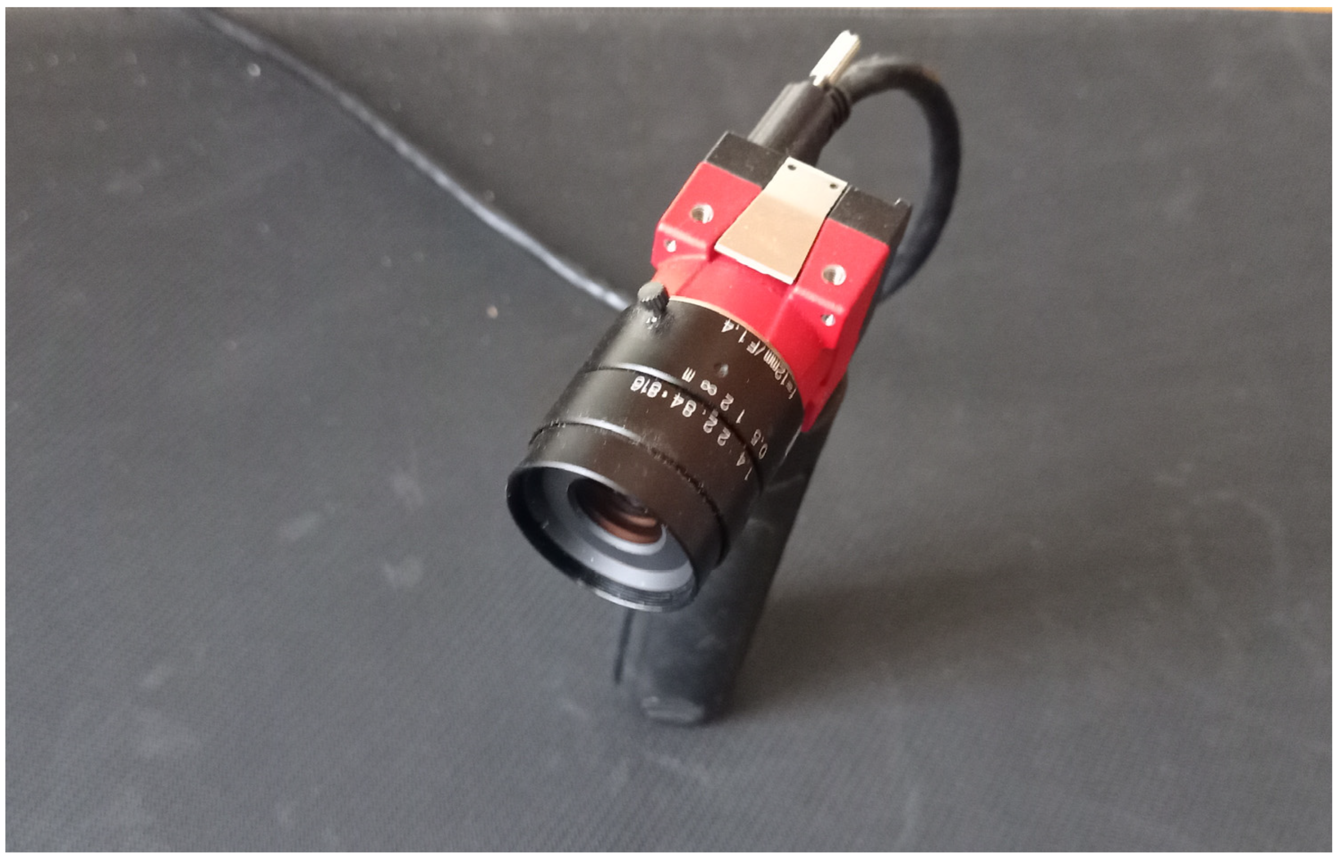
The designed vision system comprises a camera and a PC-based image processing unit. The following models were considered to select the camera: GO-5000-PGE with GigE Vision, LENS BASLER C23-1618-5M, and Alvium 1800 U-050. These models proved efficient in industrial applications during the previous project conducted by the author. However, the GO-5000-PGE and LENS BASLER C23-1618-5M models demand additional equipment to transfer images between the camera and the processing unit. The GO-5000-PGE needs a Gigabit PCI Express Network Adapter, while the LENS BASLER C23-1618-5M requires a dedicated frame grabber card. Only the Alvium 1800 U-050, manufactured by Allied Vision, can be directly connected to the USB3 interface. Since this model was designed for high-performance industrial applications and enabled high-quality image acquisition, it was selected for the developed application. It runs 117 frames per second at 0.5 MP resolution, enabling high-speed communication using the USB3 Vision interface (
Figure 1). The most important technical specifications are presented in
Table 1.
The PC-based image processing system is deployed to acquire images from the camera. It utilises Intel Core i7-6700HQ CPU 2.6 GHz and 32 GB RAM. A programming implementation is derived from Vimba C++ API, delivered by Allied Vision Company. It is an object-oriented API that enables interaction with Allied Vision cameras utilising GenICam transport layer modules. Additionally, OpenCV libraries are applied for image processing and Qt libraries for graphical user interface (GUI) development.
The proposed vision system is high-speed and easy to deploy. It comprises a minimal number of elements and facilitates high-quality image acquisition. However, some real-time applications may demand a higher acquisition rate. In those cases, the communication interfaces based on the GigE Vision protocol seem more suitable.
2.2. Dataset
The dataset was collected using the designed vision system. It includes 3994 images of eleven classes: Class 0 (USB), Class 1 (integrated circuit), Class 2 (fan), Class 3 (background), Class 4 (coil), Class 5 (AUX), Class 6 (USB2), Class 7 (communication unit), Class 8 (connector), Class 9 (display) and Class 10 (processing unit). The classes constitute a set of fundamental electronic components for which automatic classification is profitable for the particular manufacturing process. The process assumes that the camera is mounted 80 cm above the surface and acquires images under constant lighting conditions.
Although constant lighting conditions are assumed, the camera’s settings can influence the brightness of acquired images. Additionally, the camera’s distance from the object may need to be slightly adjusted. Therefore, the devised procedure assumes that the pictures should be collected for different distances and various lighting conditions. For this purpose, the camera was mounted at three distances from objects: 60, 80, and 100 cm, while different image brightnesses were obtained by changing the camera’s settings.
The acquired images of each class were arranged in six folders:
Distance 60 cm, brighter image;
Distance 80 cm, brighter image;
Distance 100 cm, brighter image;
Distance 60 cm, darker image;
Distance 80 cm, darker image;
Distance 100 cm, darker image.
It was to protect a uniform distribution of pictures in train, validation, and test sets. If all images in the class constituted one folder, the random split could cause an unequal representation of the samples; for example, the train set could include mostly darker images, while the test set the brighter ones.
To protect against data leakage, the same object should occupy a different area of each image in the dataset. Otherwise, very similar images would exist in training and validation sets after random splitting. As a result, the model could achieve unrealistically high performances in the validation and test sets since it memorised information from the train set.
Hence, the acquisition procedure assumed that each part should be located on a grid, for which the distance between two points should be greater than 5 cm. With this assumption, given the geometrical constraints of the scene, 3994 images were acquired, approximately 360 for each class. Eleven of these images, as a sample, are presented in
Figure 2.
The dataset was divided into training/validation and testing data using the train_test_split () function from the Keras library. This division was executed for each class’ folder separately, ensuring that the data would not be derived from the same distribution during randomised operations performed in the training stage. The training procedure assumed that 80% of the dataset was selected for training/validation and 20% for test data.
The training/validation data was divided into train and validation sets numerous times during experiments. The randomness of the division was controlled using the seed parameter of the train_test_split () function. This control facilitated training each model with the same seeds and, consequently, the same train/validation split sets. That was to benchmark devised networks in comparable conditions. As a result, each model was trained ten times based on the same train/validation split sets, for which 75% of the train/validation data was for training and 25% was for validation.
The test data was finally used to compare the best models in the research’s closing step. The adapted division is the most common attempt to deal with the fundamental issue in machine learning, which is the tradeoff between optimisation and generalisation. Optimisation refers to adjusting a model to get the best performance on the training data. In contrast, generalisation refers to how well the trained model performs on data it has never seen before. The goal is to get good generalisation without controlling it; therefore, the model should be fitted using only its training data. If the model is fitted too well, overfitting appears, and generalisation suffers.
2.3. Baseline Model
A baseline model helps to understand the data indicating if the data is insufficient or inadequate for the formulated task. It also constitutes a benchmark for more complicated models, providing baseline metrics that can be used as a reference point throughout development. Due to its simplicity, it is easy to develop and test in a relatively short time.
The adopted baseline model represented the most straightforward neural network architecture that achieved statistical power.
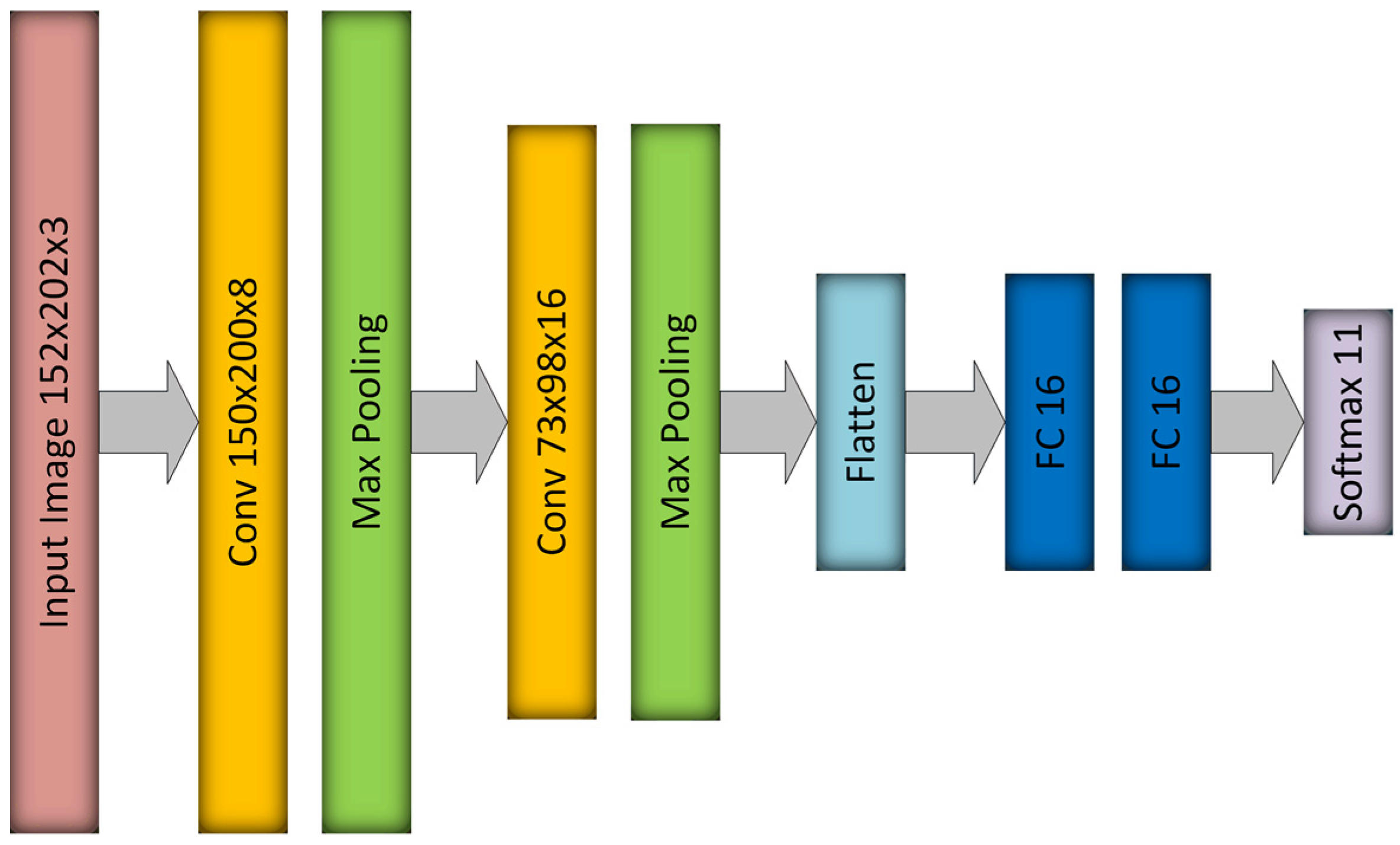
Figure 3 shows the established structure that constitutes the most common approach for designing convolutional networks. It consists of two convolutional layers and two dense layers. After each convolutional layer, pooling layers are inserted. They downsample feature maps making successive convolution layers look at increasingly large windows. A flatten layer succeeds the second pooling layer to reduce the spatial dimensions of the input into a vector. This operation facilitates employing a dense layer, which is subsequently connected to a softmax layer. The baseline model architecture is presented in
Table 2.
The designed training procedure principally utilises default parameters implemented in fit () function of the Keras library. Namely, the training was carried out using an Adam optimiser with a learning rate equal to 0.001. The batch size was set to 32 (a more significant size caused memory shortage), the epoch number to 200, and the shuffle parameter to True, which meant that the order of images was randomly changed at each epoch. The initialisation of the network weights was performed using the Glorot uniform initialiser.
The size of the output images from the camera is 608 × 808 × 3 pixels (RGB format). It is too large to process by neural networks due to the high computational cost. Since the default size of the input image of most state-of-the-art networks is 229 × 229 × 3 pixels, the input image size was set to 152 × 202 pixels (to preserve the ratio). Additionally, the pixel values were normalised between 0 and 1 since this normalisation constitutes the standard procedure applied to input images.
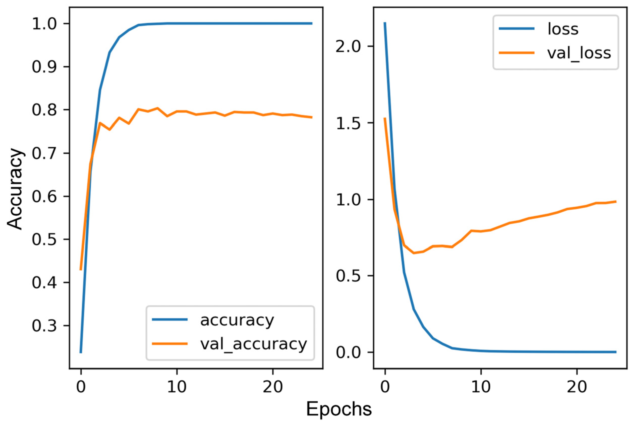
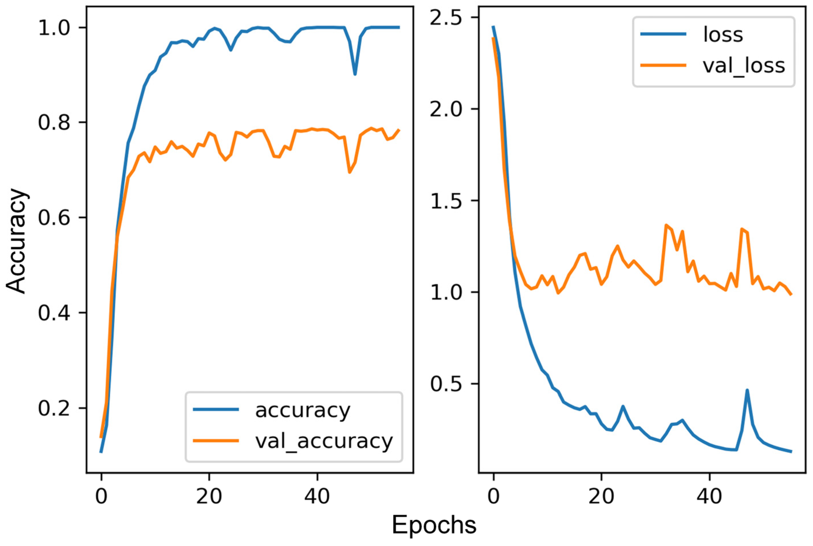
Classification accuracy was adopted to evaluate the measure of success because each split contained a similar number of samples from each class. Consequently, the learning curves of accuracy and loss were used to analyse the performance of designed networks. In
Figure 4, the learning curves for the baseline model are presented. They suggest that the model can learn using training data, proving that the dataset is sufficiently informative and that the network predicts classes for given input data. Additionally, it confirms that the adopted network architecture is appropriate for the classification task and that data leakage does not exist since validation loss is higher than train loss. Nevertheless, the model exhibits high variance and overfits after the fourth epoch. Two solutions can be employed to deal with these issues: additional data and regularisation.
Extending the dataset seems to be very challenging. Additional images could be very similar to the ones already included in the dataset. As a result, data leakage between train and validation sets could occur. Therefore, the regularisation techniques were investigated, such as data augmentation, dropout, and weight regularisation.
Data augmentation is a powerful technique for mitigating overfitting in computer vision, which generates more training data from existing training samples via random transformations. There are two approaches to data augmentation: data expansion and in-place data augmentation. Data expansion enlarges the number of images in the dataset, while in-place augmentation modifies each image before passing it to the input layer. As a result, in-place augmentation guarantees that the model never sees the same picture twice at training time.
Since in-place augmentation constitutes a more popular technique, it was chosen for further experiments. Its programming implementation is straightforward in the Keras library since it delivers the ImageDataGenerator class. However, it demands defining various parameters, which should be employed during image transformation. Therefore, through experimentation, the following set of parameters for the generated dataset was determined:
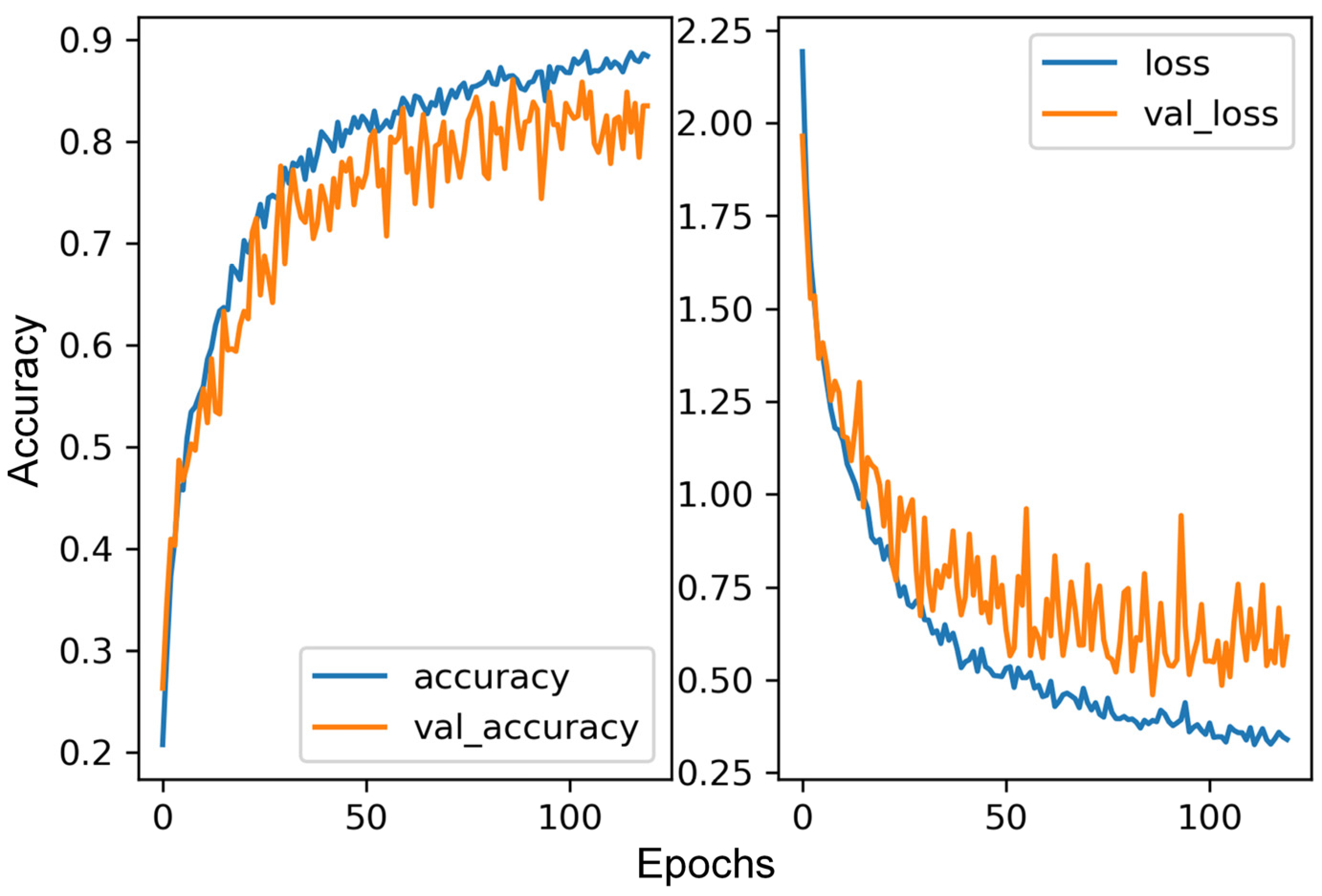
The result of applying data augmentation for the baseline model (
Figure 5) suggests that the network’s capacity is insufficient, and the model cannot improve performance using augmented data. Consequently, the dropout technique was examined.
Dropout is a very effective and commonly used regularisation technique. It is applied to a layer to drop some output features during training randomly. As for data augmentation, Keras facilitates the simple implementation of this technique, which was utilised here (dropout = 0.5). However, the obtained results, as with data augmentation, indicated the insufficient capacity of the network to learn dataset representation (
Figure 6).
The last analysed technique was weight regularisation, which adds a cost associated with large weights to the model’s loss function. The added cost can be proportional to the absolute value of the weight coefficients (L1 norm) or the square of the weight coefficients value (L2 norm). Taking advantage of the simple implementation of this technique in Keras, both norms were applied to the baseline model.
Figure 7 presents the learning curves for better performance (L2 = 0.001). They also point out the incapability of the network to learn from train data.
Although the developed model proved that the dataset is sufficiently informative and the network predicts classes given input data, it appeared too simple to apply regularisation techniques. Therefore, further research was devoted to developing a more complicated custom model that could reduce overfitting by utilising regularisation techniques.
2.4. Custom Models
Custom models were designed by increasing the complexity of the baseline model by adding convolutional and dense layers of different sizes. To find the optimal network structure, ten models of various complexity were investigated (
Table 3).
2.5. Pretrained Networks
Since fine-tuning demands a larger dataset, feature extraction was selected for pre-trained network investigations. Based on the literature review, the most promising network architectures were chosen:
VGG16;
VGG19;
ResNet50;
Xception;
InceptionV3.
The dense layers of the above networks were replaced with new classifiers. Five classifiers of different sizes were designed (
Table 4) and tested for each model to find the optimal structures. Additionally, an image processing step was employed. It was because adopted networks expect different image formats at the input layer. For example, VGG16 demands images converted from RGB to BGR and a zero-centred colour channel. This operation, as well as the programming implementation of the pre-trained networks, is very straightforward using the
applications module of the Keras library.
3. Results
To develop an electronic components classification method based on convolutional neural networks, the most promising models were designed in the previous section. In this section, the proposed models are evaluated. For this purpose, numerous experiments were performed. Firstly, the different custom model structures were trained, and their performances were assessed using accuracy rates and learning curves. In the same way, pre-trained models with different classifiers were analysed. Finally, a comparative analyse was performed using the most promising custom and pre-trained models to find the best network for the classification task.
Due to the stochastic nature of deep learning models, each network was trained ten times, and the mean accuracy was considered. Each of the ten training steps was performed with a different random seed value (random split of train and validation sets). However, the same ten training steps were deployed for all networks. Consequently, each network was trained with the same random seed values and hence with the same random splits of the dataset into test and validation sets. This procedure ensured the same training conditions for the analysed models. For final analyses, each chosen model was trained three times using the same random seed, and the best performance was evaluated.
Each training step utilised a checkpoint mechanism. It allowed saving the network’s weights if the achieved accuracy at the epoch’s end was higher than the previously recorded one. In this way, the best models obtained during training were saved.
3.1. Custom Network
The custom networks constitute more complex structures of the baseline models. Since the baseline models exhibited overfitting, the custom networks were trained using regularisation techniques. Firstly, data augmentation was applied.
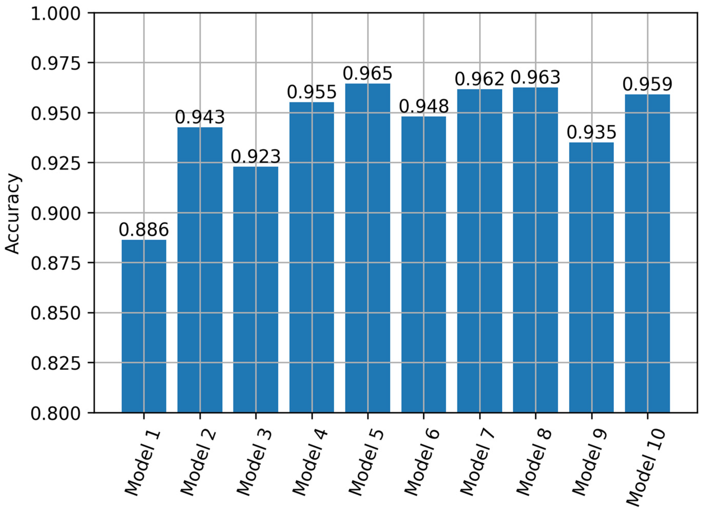
The results suggest that increasing the models’ complexity somewhat influences the performance (
Figure 8). Admittedly, the simple models 1–3 achieved slightly smaller accuracy, but the very complex models 7–10 did not outperform the others. Model 4 was the simplest one that achieved 96% accuracy.
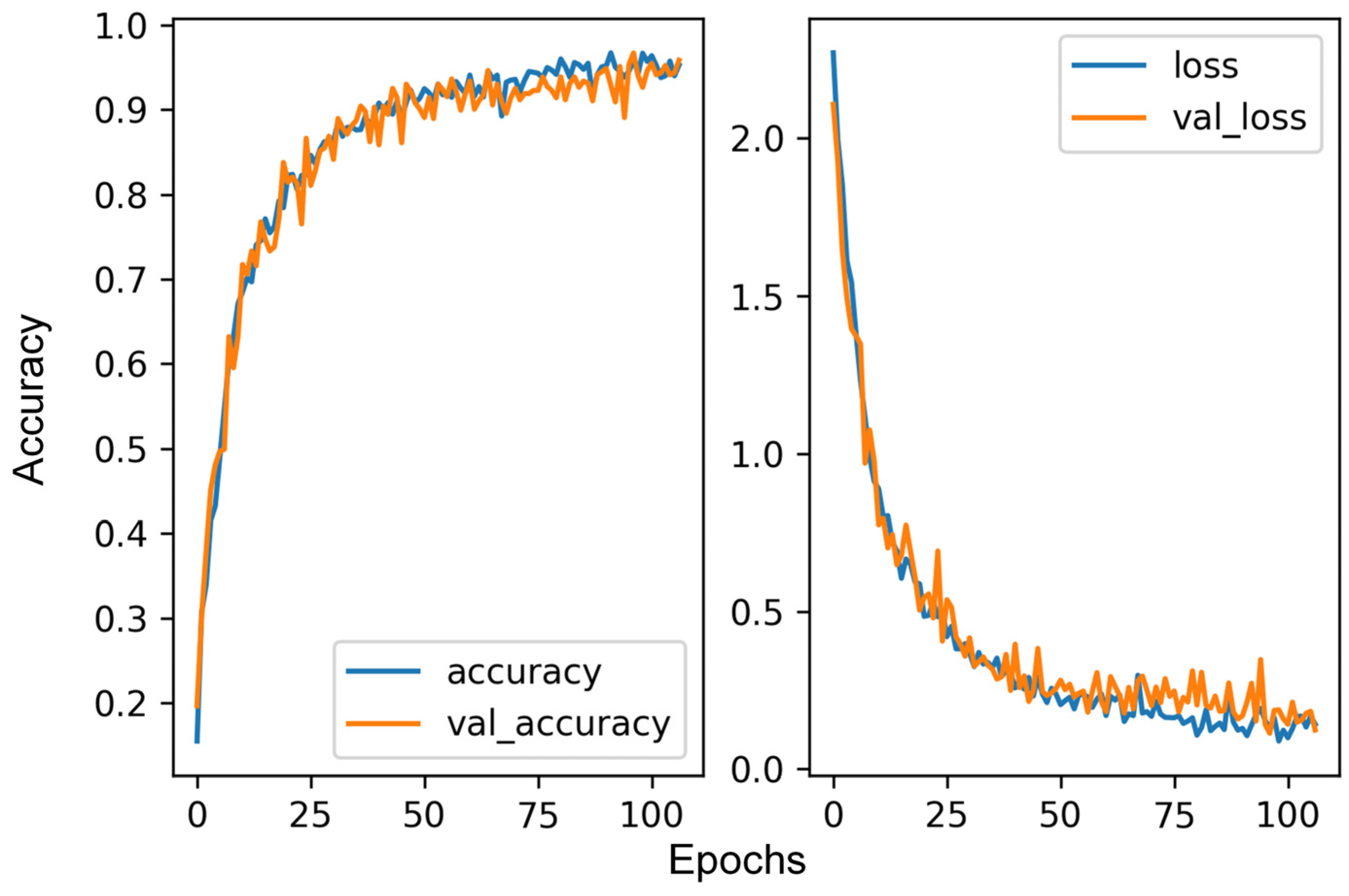
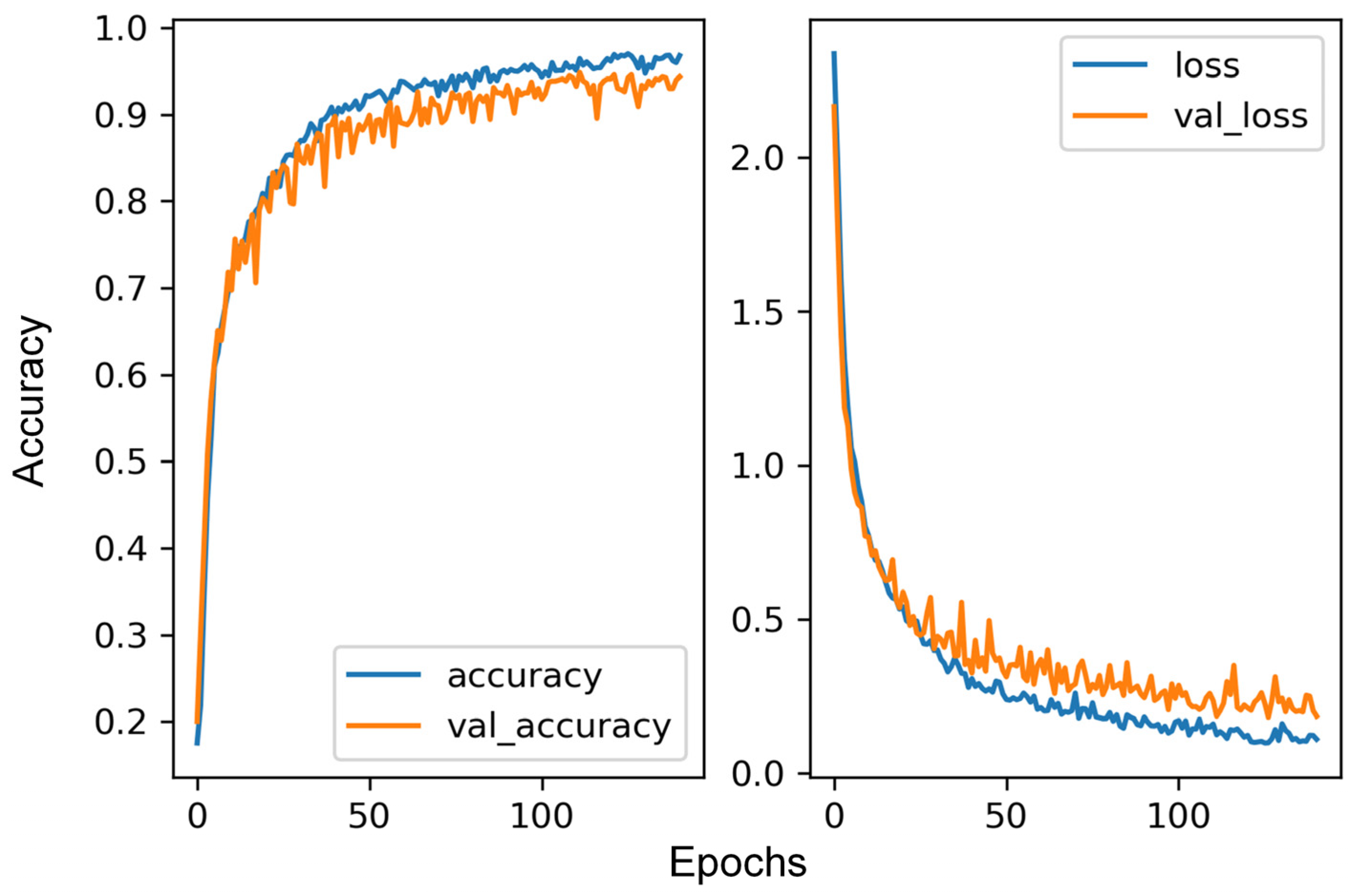
Its learning curves prove a positive effect of data augmentation on the training process (
Figure 9). The variance and overfit present in the baseline model were successfully removed. The model needed 105 epochs to learn in 1950 s.
The subsequent experiments were devoted to testing dropout and weight regularisation methods. For this purpose, the dropout layers with a 0.2 drop coefficient were implemented in the dense layers. The results indicate that this technique is not as successful as data augmentation. The best model (Model 7) achieved only 82% accuracy. The higher dropout coefficient slightly improved the networks’ performance. For the 0.5 drop value, the best model (Model 7) achieved 88% accuracy. For weight regularisation, the results were similar. The best model (Model 5) attained 83% accuracy for regularisation coefficient L1, equalled 0.001. Other values of the regularisation coefficient resulted in poorer performance.
3.2. Pre-Trained Networks
The dense layers of the analysed structures were replaced with the designed classifiers to investigate the pre-trained networks. Consequently, five models of various complexities were considered. Each model was trained ten times with arranged different test/validation splits. For comparison, the same splits were deployed for each network.
3.2.1. VGG16
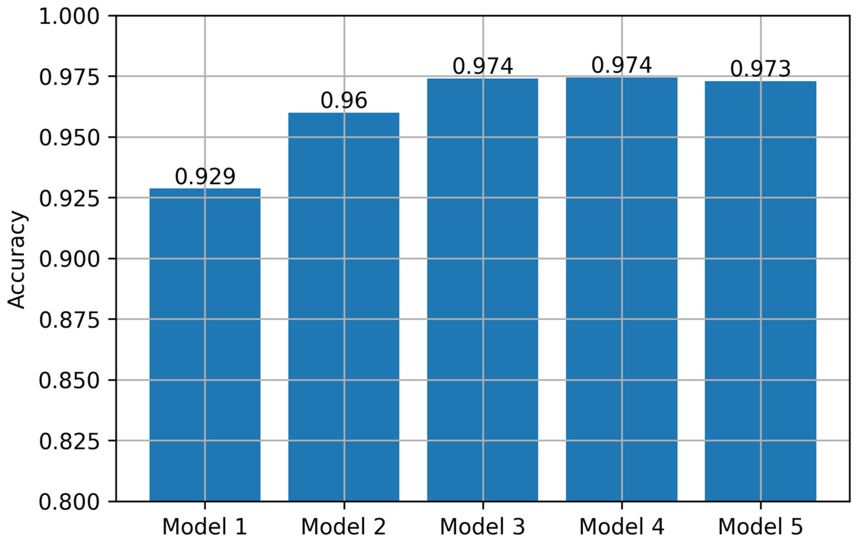
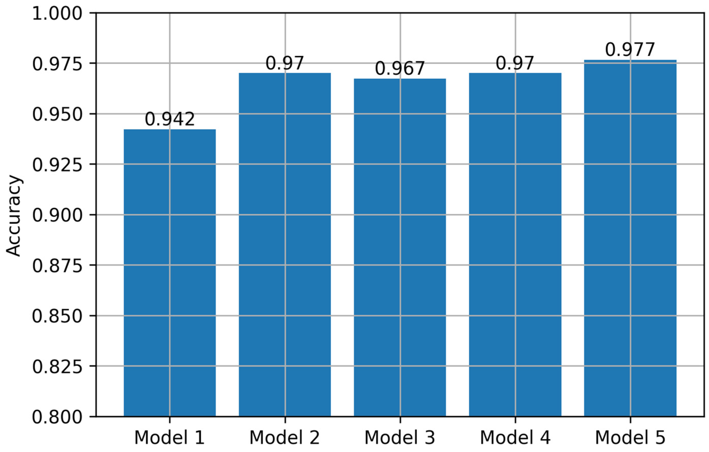
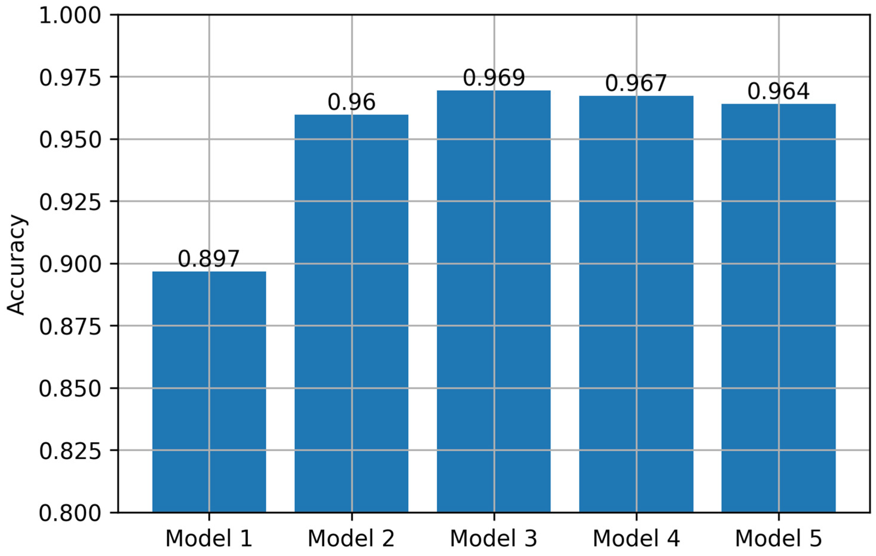
Figure 10 illustrates the results obtained for the VGG16 network. They indicate that only the network with the simplest classifier achieved worse accuracy (93%). The rest model performed similarly, achieving comparable accuracies.
The generated learning curves (
Figure 11) suggest that overfitting is not presented in this model; however, some variance related to the gap between both curves occurs. Therefore, similarly to the previous experiments, the regularisation techniques were deployed.
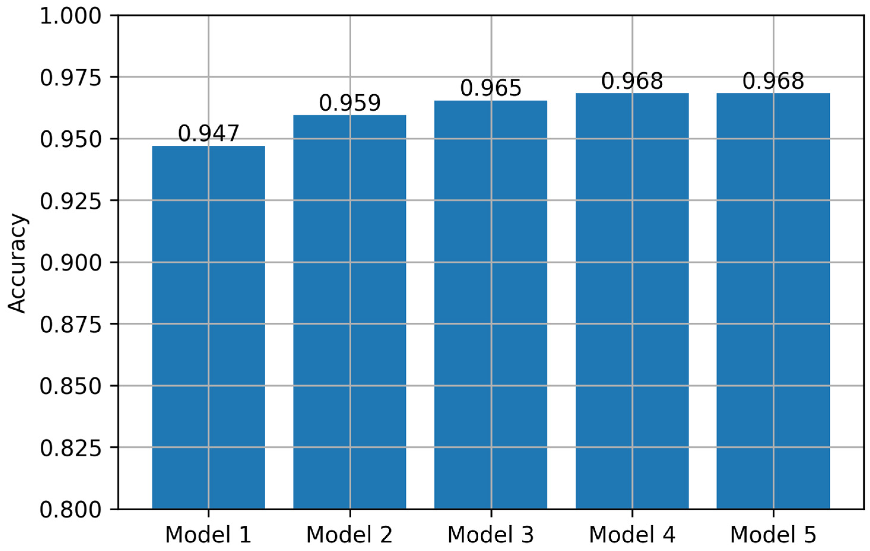
Data augmentation yielded only a slight improvement in accuracy (
Figure 12). However, it contributed to variance reduction, as seen in
Figure 13 (results obtained from Model 2). The dropout technique was effective only for Model 5 (96% accuracy), while the rest models were not capable of learning. The models generated similar results for weight regularisation, as presented in
Figure 10.
3.2.2. VGG19
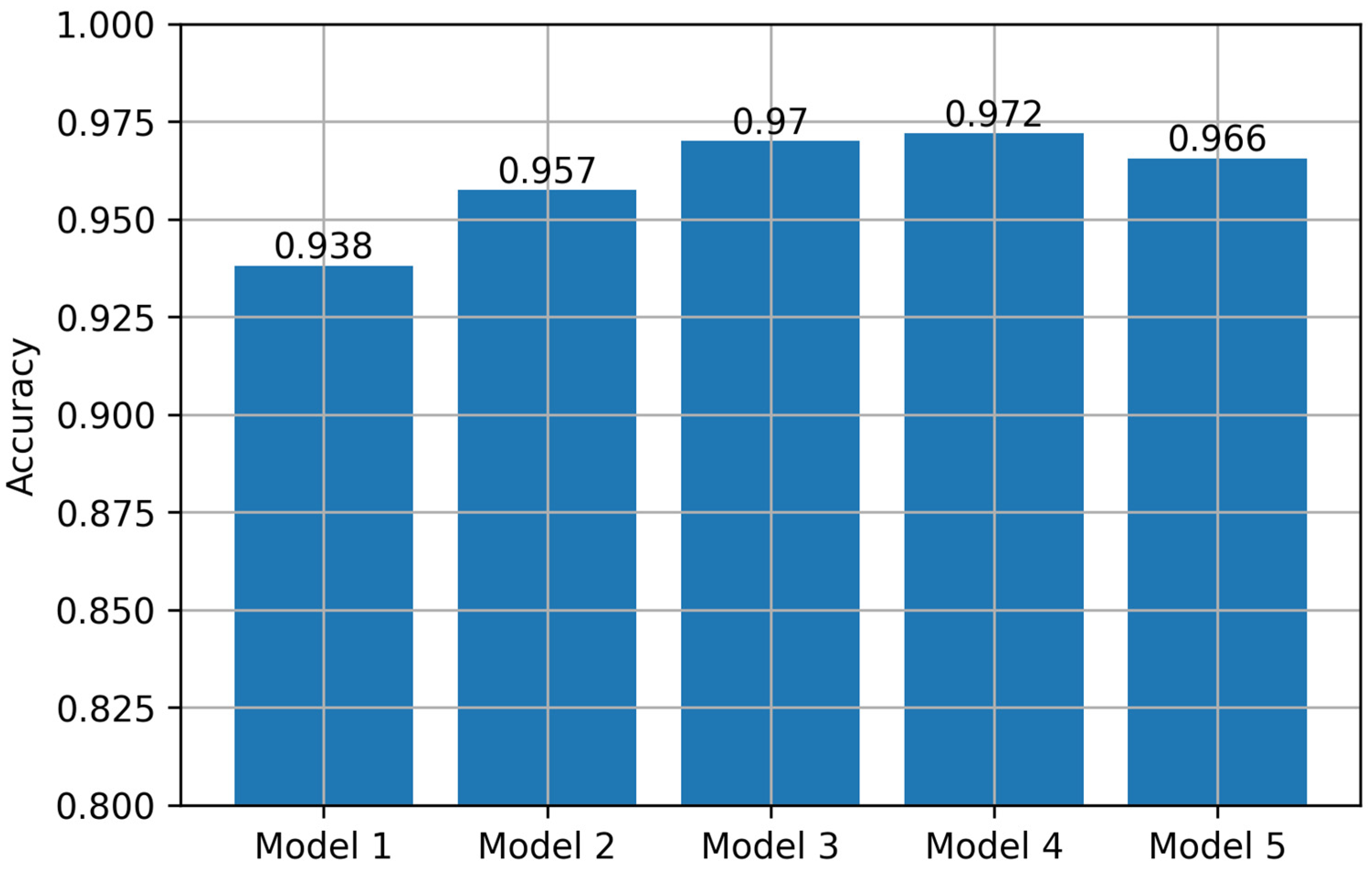
VGG19 exhibited a slightly poorer performance than GG16. The simplest classifier yielded the lowest accuracy, while the rest performed similarly (
Figure 14).
The implementation of regularisation techniques resulted in a similar performance as for VGG16. Dropout and weight regularisation led to 96% accuracy for the best model (Model 5). Data augmentation slightly improved the results presented in
Figure 14 (see
Figure 15). In this case, more complex models achieved 97% accuracy.
3.2.3. ResNet50
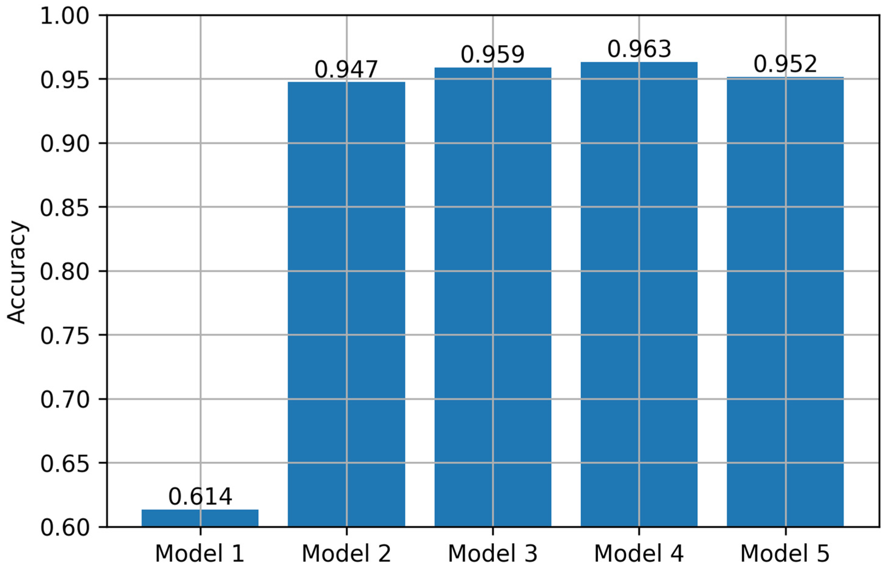
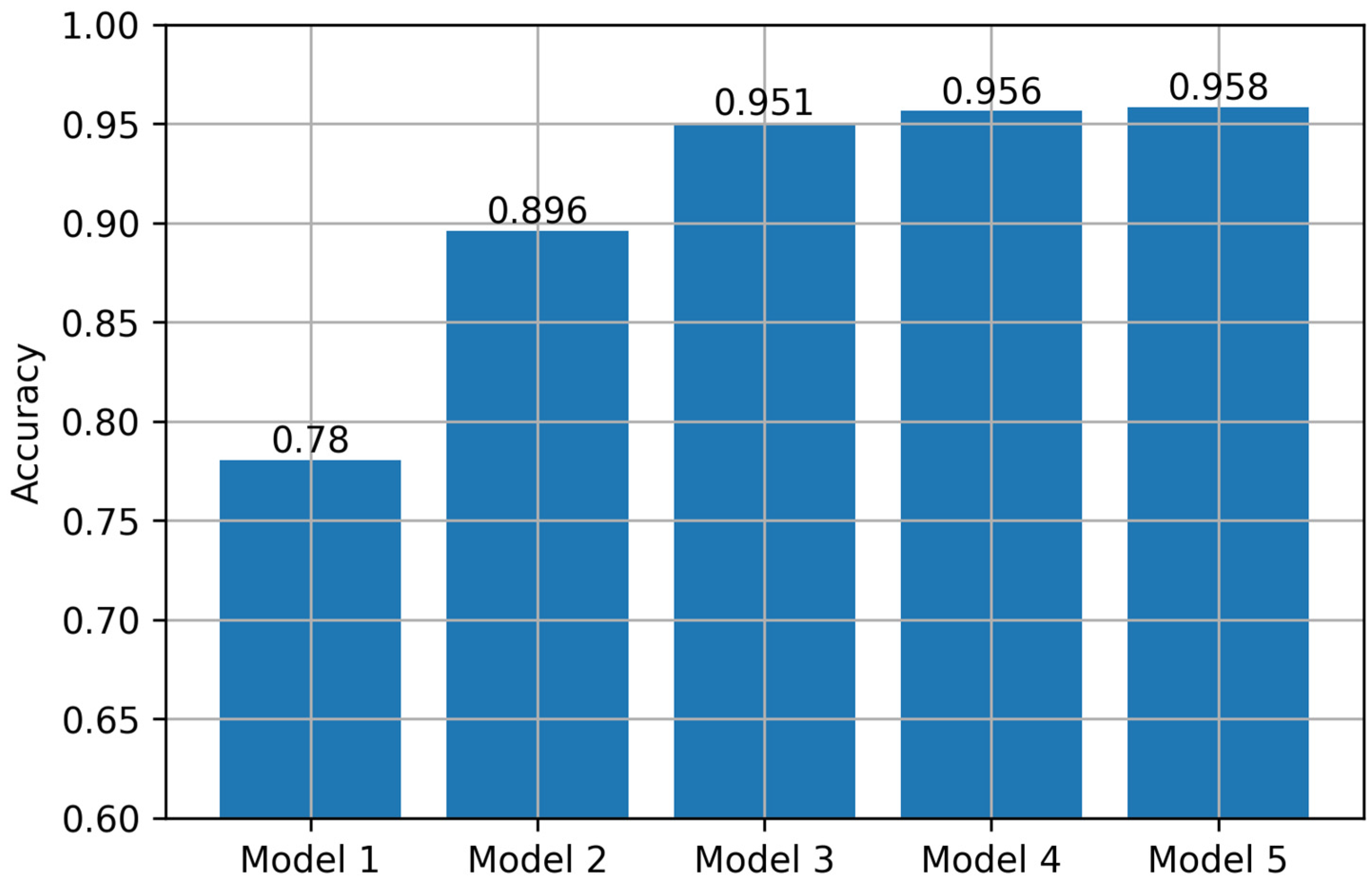
ResNet50 achieved similar performance as previous networks. Only the simplest model presented lower accuracy, equal to 61% (
Figure 16).
The regularisation techniques also had a minor impact on the ResNet50 performance. Data augmentation slightly increased accuracy for all models (
Figure 17), while the application of dropout and weight regularisation improved the performance of the simplest model (Model 1). The more complex networks obtained similar results as in the case of data augmentation.
3.2.4. Xception
Xception performed similarly to VGG16, VGG19 and ResNet50 (
Figure 18). In this case, the simplest model achieved the better result. The augmentation technique influenced only Model 1 and Model 5, increasing accuracy slightly (
Figure 19). Dropout and weight normalisation did not improve the performance. For both techniques, only Model 5 achieved 96% accuracy.
3.2.5. InceptionV3
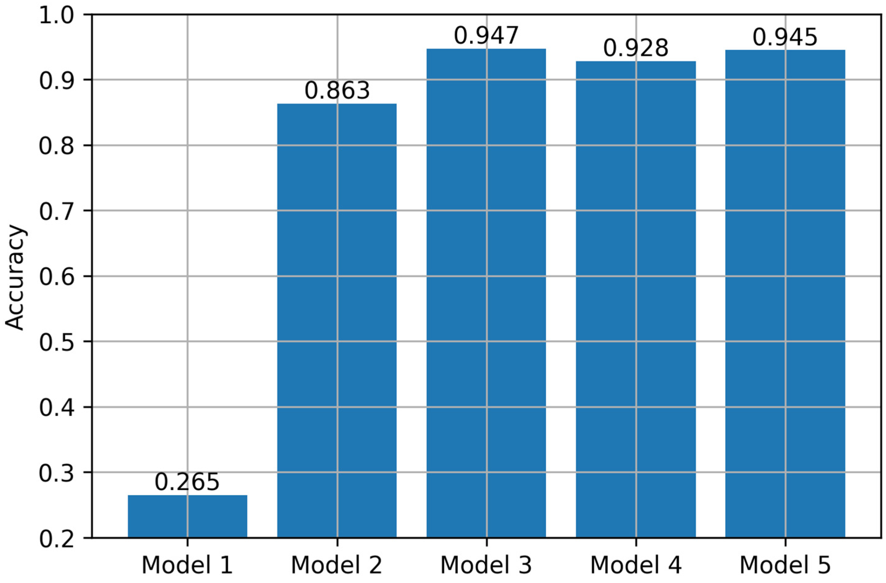
The most complex models (Model 3–5) of InceptionV3 achieved similar results as the above networks (
Figure 20). However, as opposed to previous networks, data augmentation impaired performance (
Figure 21). Consequently, the most complex models (Model 4 and 5) reduced their accuracy to 93% and 94%, respectively.
The network was not able to learn using the dropout method. Nevertheless, it achieved similar results for weight normalisation to those presented in
Figure 20.
3.3. Comparison of the Most Accurate Models
To find the most promising structure, the following models were chosen for final comparison: the custom network (Model 4), VGG16 (Model 5), VGG19 (Model 3), ResNet50 (Model 3) and Xception (Model 3). Each model was trained three times on all the available data (training and validation) and evaluated on the test set. Apart from accuracy, training time and execution time (calculated for classifying 3172 images in the train/validation set) were considered. The obtained results for the best performance of each network are presented in
Table 5.
The results suggest that all the pre-trained models outperformed the custom network. Nevertheless, the difference between the best and the worst amounted to only 1.22%. The confusion matrix of ResNet50 performance (
Figure 22) shows that the network did not correctly classify objects only in individual cases.
Regarding time, the custom network proved to be the fastest one. It was trained at least two times faster than other networks. Additionally, the execution time was considerably shorter. Compared to ResNet50, the custom network could classify objects almost five times faster. The training time is not crucial since the database preparation is more time-consuming. However, the execution time can be essential for the processes that demand deploying fast-speed cameras.
4. Discussion
The present work focuses on developing a method for electronic component classification in a specific process. It considers all necessary steps, such as image acquisition, database creation, and neural network development. This approach differs from the previous research, where generic databases were utilised. These databases mainly included images of elementary components from various technological processes.
The image acquisition system was proposed in the first step of the experiments. Based on this, the database was developed. The created baseline model proved the suitability of the proposed database and validated the assumption for the custom neural network structures. Utilising the baseline model, more complex custom networks were created. They were subsequently trained using various regularisation techniques. The results showed that data augmentation outperformed dropout and weight regularisation in most experiments. It also proved to be effective in the case of pre-trained networks.
As pre-trained networks, the most promising structures were chosen. Then, their dense layers were replaced with the designed classifiers, and the new structures were trained using the same train/validation splits. The results suggested that the classifiers built of two dense layers with 64 neurons and a softmax layer were sufficient in most cases. Among the tested networks, ResNet50 achieved the highest accuracy (99.03%), but the worst one (VGG19) obtained a slightly worse result (97.81%).
The custom network attained the worst accuracy (96.59%). It may result from the fact that a complex convolutional base of pre-trained networks can detect more distinctive features than plain convolutional layers of the custom network. In this regard, a more sophisticated custom model could be investigated. However, since ResNet50 obtained very high accuracy, developing a model that could perform even better seems challenging. Moreover, the custom network’s less complex structure results in faster performance. This property may be usable in technological processes utilising fast-speed cameras.
The results suggest that pre-trained networks are more suitable for electronic component classification in the designated application, which is in line with the previous research [
26]. However, some studies [
28,
32] have proved the better performance of custom networks. It could be because the authors utilised different databases to classify different components.
5. Conclusions
In this paper, the problem of classifying electronic components in industrial applications has been addressed. The results suggest that the solution based on the ResNet50 architecture achieved the highest classification accuracy (99.03%), which is better than the 98.99% attained in relevant research on classifying elementary components.
However, the previous research generally focused on utilising accessible databases to develop neural network structures for classifying mostly elementary objects, such as resistors, capacitors, diodes and integrated circuits. Additionally, the authors mainly introduced the final classification models without presenting intermediate development steps or training details. This approach is convenient when all researchers use the same database, e.g., ImageNet, for classification performance comparison. Nevertheless, in the case of industrial applications, it can be expected that each classification task may demand a distinct dataset.
Consequently, this research investigates all essential issues of building a classification system, such as image acquisition, database creation and neural network development. All of the above steps are described in detail to allow other researchers to replicate and modify them. Additionally, the code and dataset are published for easy implementation.
The proposed solution is dedicated to technological processes, characterised by constant lighting conditions, a fixed camera position and a designated set of classified components. However, many computer vision applications can deploy the above conditions. For example, a video surveillance system in indoor places may leverage the present method for object classification tasks.
It should be noted that this research considered only a straightforward model of a custom network. More sophisticated structures based on residual or inception networks can be as accurate as pre-trained models but significantly faster. Since they may be especially suitable for technological processes utilising fast-speed cameras, future work should focus on applying a classification system in high-speed applications.
