Intelligent Identification Method for Drilling Conditions Based on Stacking Model Fusion

Abstract

Due to the complex and changing drilling conditions and the large scale of logging data, it is extremely difficult to process the data in real time and identify dangerous working conditions. Based on the multi-classification intelligent algorithm of Stacking model fusion, the 24 h actual working conditions of an XX well are classified and identified. The drilling conditions are divided into standpipe connection, tripping out, tripping in, Reaming, back Reaming, circulation, drilling, and other conditions. In the Stacking fusion model, the accuracy of the integrated model and the base learner is compared, and the confusion matrix of the drilling multi-condition recognition results is output, which verifies the effectiveness of the Stacking model fusion. Based on the variation in the parameter characteristics of different working conditions, a real-time working condition recognition diagram of the classification results is drawn, and the adaptation rules of the Stacking fusion model under different working conditions are summarized. The stacking model fusion method has a good recognition effect under the standpipe connection condition, tripping in condition, and drilling condition. These three conditions’ accuracy, recall rate, and F1 value are all above 90%. The stacking model fusion method has a relatively poor recognition effect on ‘other conditions‘, and the accuracy rate, recall rate, and F1 value reach less than 80%.

1. Introduction

Drilling engineering is one of the essential links in petroleum exploration and development operations. With the development of deepwater and unconventional oil and gas fields, the risks related to well control during drilling are increasing [1]. Due to the limitations of the existing formation pressure prediction method and drilling process, it is still impossible to completely avoid the intrusion of formation fluids [2,3,4]. For the safety of drilling operations, the timely identification of drilling conditions is important for the implementation of well control programs [5,6,7]. Affected by the complexity and unpredictability of the formation, a large amount of logging data needs to be processed during the drilling process to optimize drilling, reduce costs, and increase efficiency [8]. Drilling conditions are complex and varied, including round-tripping, standpipe connection, drilling, drilling cement plug, cementing, and circulation [9]. In different periods, identifying different drilling conditions is the basis of overflow intelligent identification and analysis [10]. The drilling operation status can be analyzed in real time by identifying the drilling conditions to improve drilling efficiency and reduce costs [11].

The current drilling condition recognition methods are divided into two aspects: threshold judgment based on empirical evidence and intelligent recognition based on data-driven machine learning. Threshold judgment based on experience recognition is mainly based on expert experience and physical models to realize the diagnosis of drilling conditions [12]. Based on the data-driven machine learning method, the problem of condition recognition is transformed into a classification problem by modeling a large number of historical data or a large number of real-time data. The recognition model is obtained by continuous training [13]. In recent years, with the development of big data and artificial intelligence technology, the real-time and intelligent recognition of drilling conditions has attracted increasing attention [14,15]. Most of the research hotspots focus on the real-time identification of drilling conditions based on drilling parameters, combined with expert experience and machine learning.

Using the threshold method, Chen [8] modeled the flow of 10 working conditions in the drilling process based on the variation in drilling parameters and analyzed the drilling process over time, which improved the drilling efficiency of a single well to some extent. Sun et al. [15] proposed a real-time recognition method for drilling conditions based on support vector machines (SVM), established an SVM recognition model, and compared different kernel functions of the SVM recognition model to train the optimal model parameters. This method reduces the uncertainty and subjectivity of manual identification of drilling conditions and improves adequate drilling time. Sun et al. [16] proposed a drilling overflow identification method based on long and short-term memory (LSTM) networks using logging data, which improved the accuracy of overflow risk identification during the drilling process. Du [17] performed a real-time diagnostic analysis of overflow risk by constructing a BP neural network model and a random forest model based on drilling parameters that vary significantly when overflows occur. Yin et al. [18] performed the intelligent identification of drilling operations through mathematical statistics and manual empirical models. Based on the identification of the working conditions, the daily operating time and the total operating time of drilling operations are carefully divided.

Based on actual drilling data, Wang [19] used wavelet decomposition and reconstruction methods to eliminate the trend of data changing with well depth, remove the noise caused by sensor measurement error, and obtain the data trend in time series. Six standard drilling working states were identified by the 1D convolutional neural network combined with the Bidirectional GAN (BiGAN) algorithm. Chiranth et al. [20] proposed a method based on Stacking learning to predict drilling speed. Firstly, the three physical prediction models of Bingham, BY, and Motahhari were compared, and the parameters such as rotational speed, weight on bit, and rock strength related to drilling speed prediction were analyzed. The predictions of all base learners were output by the Stacking integration method using three physical models and the random forest model and K-nearest neighbor (KNN) as base learners. The weights of the recognition results of different algorithms are adjusted by comparing the magnitude of the test set errors to finally achieve the optimal weights. Jared et al. [21] used five base learners, linear regression, quadratic Poisson regression, support vector machine regression, random forest, and gradient boosting for production prediction with a production dataset from small-sized unconventional reservoirs. They compared four integration strategies, the direct evaluation of prediction results, weighted evaluation, neural network stacking, and random forest stacking model, in which the random forest stacking model had the highest accuracy. Cai [22] applied random forest, the gradient boosting decision tree (GBDT) algorithm, and the eXtreme gradient boosting (XGBoost) algorithm as base learners to fuse the Stacking model given the lack of a corrosion data set for offshore oil and gas pipelines and the undefined index of influencing factors. Different weights are given according to the prediction effect of the base learner, and the weighted average is used as the input feature of the Stacking two-layer algorithm. The algorithm can fit the corrosion rate of offshore oil and gas pipelines and expand the pipeline corrosion data set. Qin et al. [23] proposed a weak learner with a better fluid identification effect using an integrated decision tree, support vector machine, random forest, and GBDT. Based on the Stacking model fusion method, the fluid logging dry layer, gas layer, gas–water layer, and water layer response characteristics of high-temperature and high-pressure reservoirs in Yinggehai Basin were identified. The accuracy and robustness of the model fusion fluid identification method were better than a single model. Zhao et al. [24] used the k-means clustering method to normalize the field data for well-kick risk prediction by combining it with four artificial neural networks. Among them, the regularized radial basis function neural network (RBFNN) + k-means model had the highest prediction accuracy.

It is crucial to ensure the reliability of the discrimination results in anomaly discrimination, and the warning reliability of a single diagnostic system is poor [8,25]. In addition, the logical threshold discriminant method is highly subjective and error-prone [14]. To address the shortcomings of a single identification method, this paper proposes an ensemble learning multi-classification method based on Stacking model fusion. By training a variety of logging parameters, the real-time identification of drilling conditions is realized, which lays a foundation for overflow warning and monitoring under different working conditions.

2. Materials and Methods

2.1. Division of Different Working Conditions and Changes in Characteristic Parameters in the Drilling Process

In the current field operation, the artificial division of the drilling process through the recording parameters is subjective, and it is a prerequisite for the automatic identification of the working conditions to clarify the changes in the signs and response patterns of different parameters under different working conditions. Based on the drilling diary and previous summary, this paper analyzes the parameter changes under seven working conditions, such as standpipe connection, tripping out, tripping in, Reaming, back Reaming, circulation, drilling and other conditions. Other working conditions, such as drilling cement plugs and installing blowout preventers, are attributed to ‘other‘. Based on the parameters that change most directly and obviously under different working conditions, a total of eight parameters, weight on bit (WOB), rotary torque (TQ), rotary speed (RPM), standpipe pressure (SPP), hook load (HKL), mud flow out (MFO), depth bit (DBTM), and depth hole (DME), were selected to identify the working conditions.

In general, there are corresponding changes in the logging parameters under various drilling conditions, called sign changes under certain conditions. The drilling conditions are judged by the changes in parameters and logical relationships. According to the actual drilling conditions, this paper analyzes and summarizes the changes in parameters under various conditions.

Standpipe Connection: In the process of standpipe connection, WOB, TQ, RPM, SPP, and MFO are all zero, HKL increases, and the increased weight is approximately the weight of the single root. The bit position remains the same, and the depth is less than the borehole depth.

Round Trip: When tripping out, WOB, TQ, RPM, SPP, and MFO are all zero. HKL gradually decreases, DBTM decreases, and its depth is less than DME. When tripping in, WOB, TQ, RPM, and SPP are all zero. MFO is certain, HKL gradually increases, and DBTM increases, but is less than DME.

Reaming and Back Reaming: When Reaming, WOB, TQ, RPM, SPP, MFO and HKL are all more significant than 0, and DBTM is increasing, but the depth is less than or equal to DME. When back Reaming, WOB is 0, and torque, RPM, SPP, MFO and HKL are all greater than 0. DBTM is decreasing, and the depth is less than DME.

Circulation: During circulation, WOB and TQ are 0, RPM, HKL, and MFO are more significant than 0, DBTM is constant, and the depth is less than or equal to DME.

Drilling: During drilling, WOB, TQ, RPM, and SPP are more significant than 0, MFO is not 0, HKL decreases, and DBTM increases. Since the well depth measurement sensor is installed above the drill bit position, DBTM is slightly greater than or equal to DME.

Define the position ratio Deta: Deta is used to describe the relative position relationship between DBTM and DME during drilling. Where the expression of the position ratio is Deta = DBTM/DME, then when DBTM is less than DME, Deta < 1, and when DBTM is greater than or equal to DME, Deta ≥ 1.

Based on the above principles, the established parameter variations for different drilling conditions are shown in

Table 1. Parameter changes in different drilling conditions.

Parameters	Standpipe Connection	Tripping Out	Tripping In	Reaming	Back Reaming	Circulation	Drilling
WOB	0	0	0	0	0	0	>0
TQ	0	0	0	>0	>0	0	>0
RPM	0	0	0	>0	>0	>0	>0
SPP	0	0	0	>0	>0	>0	>0
MFO	0	0	0	>0	>0	>0	>0
DBTM	Unchanged	Decreased	Increased	Increased	Decreased	Unchanged	Increased
HKL	Increased	Decreased	Increased	>0	>0	>0	>0
Deta	<1	<1	<1	<1	<1	<1	≥1

, which describes the parameter variations under each state. The statistical parameter variation characteristics include WOB, TQ, RPM, SPP, MFO, DBTM, HKL, and Deta.

2.2. Sample Marking Method for Drilling Multi-Condition Identification

The key to drilling multi-condition identification sample marking is to describe the change in parameters in the drilling process, significantly transforming the dynamic process into the machine learning of the recognizable language. The variation in a particular parameter within the sampling interval is considered in all drilling conditions. Firstly, a threshold value is set, and when the amount of parameter change over time is more significant than this threshold value, the parameter change is considered valid. The data are marked by the logical judgment method and divided into three cases: increased, unchanged, and decreased. The parameter change is measured as follows: from the perspective of the time dimension, based on the sampling interval of the original data (such as 5 s), the rate of change is calculated and marked as +1 if the rate of change is positive, 0 if the rate of change is 0, and −1 if the rate of change is negative. In addition, in the sample data pre-processing process, the following marking methods are adopted for the parameters that need to judge the size of the values: parameters more significant than 0 are marked as +1; parameters equal to 0 are marked as 0; and parameters less than 0 are marked as −1. The characteristic of this marking method is that it can qualitatively describe the state of the parameter itself at a particular moment. These three numbers have no numerical value but only represent the state of the parameter itself. This method can avoid the feature recognition bias caused by the non-uniform dimension. The data are re-labeled concerning the parameter changes in Table 1, and the sample data markers are shown in

Table 2. Sample data change labeling method.

Parameters	Standpipe Connection	Tripping Out	Tripping In	Reaming	Back Reaming	Circulation	Drilling
WOB	0	0	0	0	0	0	+1
TQ	0	0	0	+1	+1	0	+1
RPM	0	0	0	+1	+1	+1	+1
MFO	0	0	0	+1	+1	+1	-
DBTM	0	−1	+1	+1	−1	0	+1
HKL	+1	−1	+1	+1	+1	+1	−1
DBTM-DME	0	+1	−1	−1	+1	0	+1/0

.

For the drilling process, the eight conditions considered in this paper are marked from 0–7, as shown in

Table 3. Working condition marking method.

Parameters	Standpipe Connection	Tripping Out	Tripping In	Reaming	Back Reaming	Circulation	Drilling	Other
Markers	0	1	2	3	4	5	6	7

.

2.3. Principle of Drilling Condition Identification Based on Stacking Learning with Multi-Model Fusion

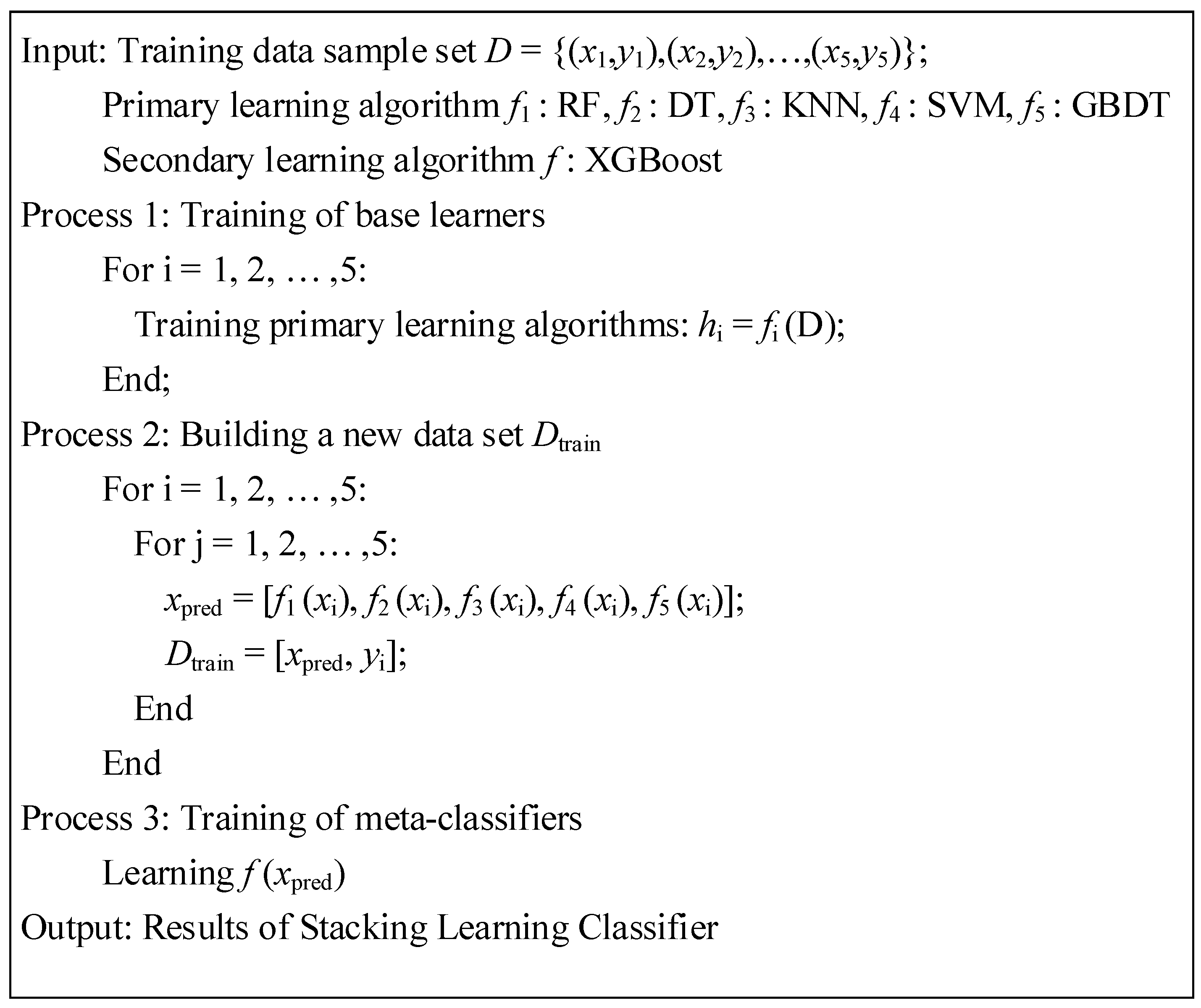
The model stacking algorithm in ensemble learning is a hierarchical multi-model fusion algorithm. The pseudo-code of the Stacking model fusion is shown in Figure 1.

Figure 1 describes a two-layer Stacking model fusion algorithm. The first layer consists of 5 base learners. The input of the base learner is the original training set, and the output is the prediction result of the base learner using the original data. The model in the second layer takes the prediction results of the base learners in the first layer as input features and adds them to the training set. These training sets are again trained in the algorithm’s second layer, and the output results are weighted to find the average.

When each base learner completes the 5-fold cross-validation, the predicted value of the current training set denoted as T1 is obtained. After this part of the operation is completed, it is necessary to predict the test set of the original data. This process will generate the corresponding predictive value pred1, which will be used as part of the next layer of the model test set. The above process is performed on each base classifier, generating T1, T2, T3, T4, and T5 for the training set data and pred1, pred2, pred3, pred4, and pred5 for the test set. The training sets of T1, T2, T3, T4, and T5 are combined to form the training set of the second layer algorithm, denoted as T. We combine pred1, pred2, pred3, pred4, and pred5 as the test set Pred for the second layer algorithm. Finally, the second layer algorithm is used to train the data output from the first layer. In drilling condition recognition, the data set is first preprocessed. Then, eight working conditions in the drilling process are finally identified by the two-layer Stacking classification method.

2.4. Multi-Classification Recognition Method Based on Stacking Learning Multi-Model Fusion

(1)

Processing of data sets

The sample data of the XX well on 23 October are used for training. The sample size in this data is O = 17266, and each sample has seven features, namely WOB, TQ, ROPA, HKL, MFOP, DBTM, and Deta. The sample matrix is X, and the shape of the sample matrix is (17266, 7). There are eight categories in total, which correspond to eight drilling conditions, namely Y = {0,1,2,3,4,5,6,7} T.

The pre-processed sample information is shown in

Table 4. Statistics of the number of sample condition categories.

Categories	0	1	2	3	4	5	6	7	Total Number
Number of samples	1103	402	93	2577	3267	1173	6656	1994	17,265

, which is the statistical information of the number of sample categories.

(2)

The implementation process of the Stacking learning algorithm based on the two-layer structure

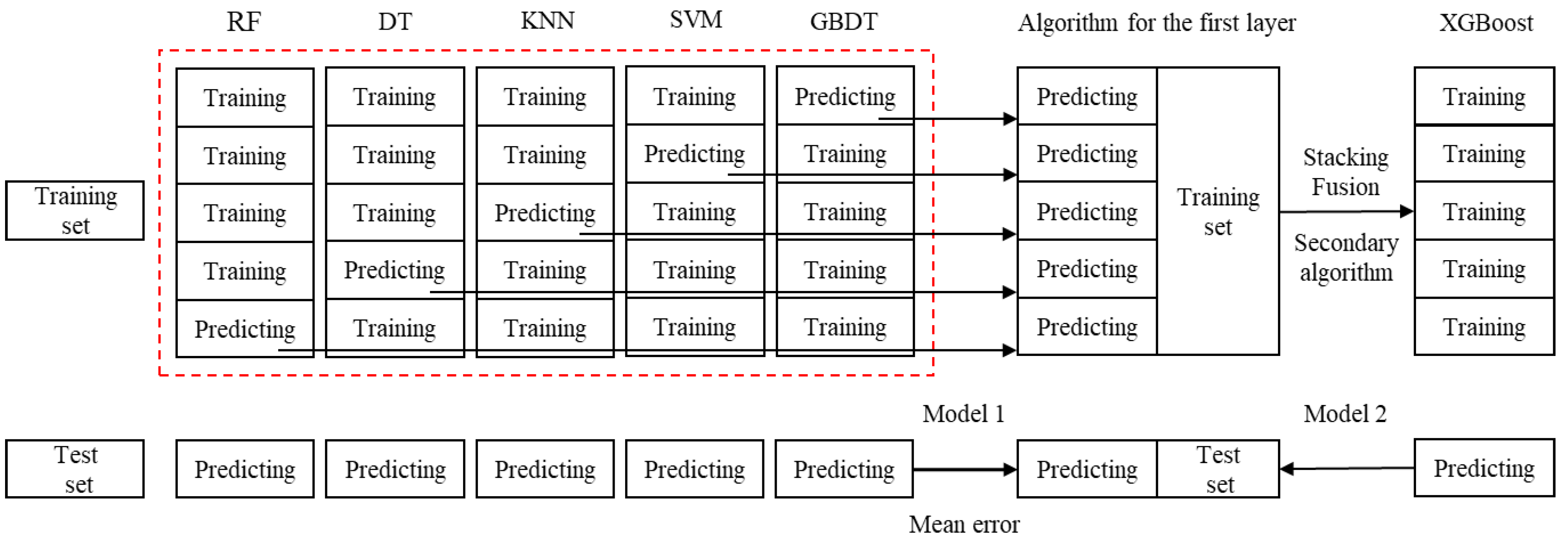
Figure 2 shows a schematic diagram of the two-layer Stacking model fusion method. During the training of the stacking algorithm, five base classifiers with two layers are used to identify the drilling conditions. The first layer uses random forest (RF), decision tree (DT), K-nearest neighbor (KNN), support vector machines (SVM), and gradient boosting decision tree (GBDT) as the five algorithms of the base learner and uses eXtreme gradient boosting (XGBoost) as the prediction algorithm in the second layer.

It can be seen from Table 4 that the category distribution of the original sample data is unbalanced. Category 6, with the most significant number of samples, is the drilling condition, with 6656 samples. Category 2, with the least samples, is tripping in, with 93 samples, and the highest ratio between samples is up to 71. Therefore, it is necessary to pre-process the sample data to achieve sample balance and normalize the original data. The SMOTE method was used to resample the samples, and in the data set partitioning, the order of the original input data was first disrupted for random sampling. The sample data set is divided into a training set X_train with a size of (11,567, 6) and a test set X_test with a size of (5698, 6), and a label result training set Y_train with a size of (11,567, 1) and a label result test set Y_test with a size of (5698, 1). In the data set Y, each label takes an integer in the range of 0–7, representing the corresponding working condition for that sample at that moment.

As shown in Figure 2, the top half represents the process of 5-fold cross-validation with different base learners, outputting the predicted values. In the 5-fold cross-validation process of the RF model, the model training process is as follows: Firstly, the 11,567 sample data of each training set X_train is divided into five parts. In each cross-validation process, 2313 × 4 data are taken for multi-classification training. After training, the remaining 2315 data are verified, the predicted value is recorded as rf_pred1, and the size of rf_pred1 is (2315, 1). The trained RF model is used to predict the test set Y_test from the original data, and the random forest classifier prediction result on the test set Y_test, denoted as rf_test1, can be obtained. The model correctness of the random forest-based learner for the first cross-validation, denoted as rf_acc1, is obtained by comparing the true label Y_test1 in the predicted dataset of rf_test1 and the original dataset. The above process was repeated four times, and the remaining 4 data were cross-validated separately. In the training process of each base learner, the training set prediction data rf_pred1, rf_pred2, rf_pred3, rf_pred4, and rf_pred5 under each cross-validation, and the test set prediction data rf_test1, rf_test2, rf_test3, rf_test4, and rf_test5 under each cross-validation can be obtained. The training set prediction data RF_pred with a size of (2315, 5) can be obtained by combining the training set prediction data by columns. For the test set prediction data rf_test1, rf_test2, rf_test3, rf_test4, and rf_test5, the test set prediction data RF_test with a size of (5698, 1) can be obtained by averaging the parts of the test set prediction data. The random forest model accuracy rate RF_acc can be obtained by averaging the accuracy of each output of the random forest model with five cross-validations. At this point, the first base learner training is completed.

Similarly, DT_pred, SVM_pred, KNN_pred, GDBT_pred, DT_test, SVM_test, KNN_test, and GDBT_test, and the accuracy of each base classifier DT_acc, SVM_acc, KNN_acc and GDBT_acc are obtained. The bottom half of Figure 2 is the model fusion section, where RF_pred, DT_pred, SVM_pred, KNN_pred, and GDBT_pred are combined into a new training data set, denoted as Stacking_train, with a size of (11,567, 5) as the training set for the second layer of the stacked model. RF_test, DT_test, SVM_test, KNN_test, and GDBT_test are combined to obtain a test set with a size of (5698, 5), denoted as the Stacking_test. In the second layer, the XGBoost algorithm is used to predict the Stacking_train and Stacking_test to complete the model fusion of multiple base classifiers and output the model’s accuracy, precision, and recall.

3. Results and Discussions

Table 5. Multi-classification confusion matrix of Stacking model drilling conditions.

Categories	Predicted to be 0	Predicted to be 1	Predicted to be 2	Predicted to be 3	Predicted to be 4	Predicted to be 5	Predicted to be 6	Predicted to be 7
0	2125				68
1		1787			108	313
2			2102	30			26
3	20	11	213	1659		35	14	196
4	21	42	3	89	1827	9		233
5		60				2148		9
6			6				2222	1
7	25	15	6	208	24	27	136	1754

shows the Stacking model drilling condition multi-category confusion matrix, which counts the number of correct identifications for each category and the number of other categories. After unbalanced processing, the total number of test set samples is 17,572. According to the confusion matrix in Table 5, the number of correct and incorrect predictions for each working condition category can be known.

The precision rate, recall rate, and F1 value of the Stacking model fusion method are calculated by the confusion matrix, and the recognition results of each working condition based on the Stacking model fusion method are summarized.

Table 6. Recognition effect of drilling multi-conditions based on Stacking model fusion.

Categories	0	1	2	3	4	5	6	7
Precision (%)	96.99	93.32	90.21	83.53	90.13	84.83	92.66	79.98
Recall (%)	96.90	80.93	97.41	77.23	82.15	96.89	99.69	79.91
F1-score (%)	96.94	86.68	93.67	80.26	85.96	90.46	96.04	79.95

shows the statistics of drilling multi-condition classification recognition results based on the Stacking model fusion method. Figure 3 shows a schematic diagram evaluating the drilling working condition recognition effect.

As shown in Table 6 and Figure 3, in terms of the accuracy of the classification model, the Stacking model fusion method has the highest accuracy rate of 96.99% for identifying the standpipe connection condition. The Stacking model fusion algorithm predicts 2191 samples in working condition 0. Among the predicted samples, the number of correctly identified cases in working condition 0 is 2125, and 66 samples of other classes are incorrectly predicted as being in working condition 0. Except for working condition 7, working condition 3 has the lowest classification accuracy rate, 83.53%. It can also be seen from the data in the table that the Stacking model fusion method predicts 1986 samples of working condition 3, of which only 1659 are correct, and 327 samples of other classes are incorrectly predicted as working condition 3.

In terms of the recall rate of the classification model, the recall rate of working condition 6 is the highest among the eight kinds of working conditions, and the recall rate is 99.69%. The points correctly identify a total of 2222 samples in condition 6, six samples are incorrectly predicted as Condition 2, and one sample is incorrectly predicted as Condition 7. The incorrect identifications may be due to parameter changes caused by the operation of other operating conditions, the unreasonable threshold setting of parameter changes, or the critical change point of the operating conditions, which causes these samples to be identified as other operating conditions. Among all of the analysis conditions, the recall rate of condition 3 is the lowest, with a recall rate of 77.23%. There are 2148 sample points, and only 1659 are correctly identified. By analogy, the evaluation indicators for other conditions are similar.

In general, the Stacking model fusion method has the lowest overall recognition ability for the samples of condition 7. The samples’ precision rate, recall rate, and F1 value reach less than 80%. The model fusion method, on the other hand, has a better recognition effect on the samples of working condition 0, working condition 2, and working condition 6, and the precision rate, recall rate, and F1 value of the Stacking model fusion method for these three working conditions all reach more than 90%. The highest precision rate is found for working condition 0, the highest recall rate is found for working condition 6, and the highest F1 value is found for working condition 0. Working condition 7 contains a variety of drilling conditions, such as leak-off tests, drilling cement plugs, and surface operations. It is difficult to describe these conditions uniformly because there is no clear pattern of parameter variation, so they are grouped under working condition 7. The Stacking model fusion method needs to classify and identify different parameter laws through supervised samples, so the recognition effect of working condition 7 with an unclear parameter variation law is relatively poor. In condition recognition, greater trust weights are given to condition 0, condition 2, and condition 6, predicted by the Stacking model fusion method.

The classification performance of the five base learners and the XGBoost algorithm is compared separately for classification recognition under the same training set and test set data. The accuracy of the Stacking model fusion method is found to be 88.91% using the Stacking confusion matrix, and the classification effectiveness of the different algorithms in drilling multi-working condition recognition applications is evaluated by comparing the classification accuracy of the Stacking model fusion method with that of the base learners. As shown in

Table 7. Comparison of the accuracy of different algorithms.

Algorithms	RF	DT	KNN	SVM	GBDT	XGBoost	Stacking
Average accuracy (%)	84.44	84.11	81.38	85.91	85.95	86.15	88.91

, the algorithm with the highest test set accuracy for the base learner was GBDT, with a maximum of 86.65%. The lowest training set accuracy is found for the KNN model, with 82.45% accuracy. The test set accuracy using the Stacking learning fusion model reaches 88.91%, which is 2.26% higher than the recognition of the XGBoost algorithm and 6.46% higher than the accuracy of the KNN model, that is, the classification recognition accuracy based on the Stacking model fusion method is higher than the accuracy of the base learner. In the classification process, the Stacking method can integrate the advantages of the base learner to improve the overall recognition of the model and achieve higher accuracy.

As shown in Figure 4, the drill bit starts drilling from 3197 m with a smooth drilling curve and then starts scribing and reverse scribing at a certain depth. The stacking fusion model-based drilling multi-conditions classification method exhibits smooth and continuous drilling curves at the folding points of the bit position curve, with few singularities. A singularity is the occurrence of isolated points identified as other conditions in a series of consecutive points. However, the accuracy, recall, and F1 values of the Stacking model fusion method for condition 7 were at most 80% because working condition 7 contains many conditions. The parameters of these conditions are very complex and need a clear pattern. In contrast, in the machine learning-based classification method, the recognition of working condition 7 requires more explicit parameter features for training.

4. Conclusions

In this paper, the oil drilling data are used for training, and the response characteristics of various parameters under different working conditions in the drilling process are analyzed. A multi-classification algorithm based on Stacking model fusion is used to identify the actual operating conditions of the XX well for 24 h. Seven conditions are considered: tripping out, tripping in, standpipe connection, Reaming, back Reaming, circulation, and drilling. Other operations are grouped into one condition: “other.” In the Stacking fusion model, the accuracy of the integrated model and the base learner is compared, and the confusion matrix of drilling multi-condition recognition results is output to verify the effectiveness of the Stacking model fusion classification model. Based on the parameter variation characteristics of different working conditions, the classification results and real-time working condition recognition diagrams are drawn, and the adaptation rules of the Stacking fusion model in different working conditions are derived. The recognition results of the Stacking model fusion method are better for the samples of condition 0, “standpipe connection condition”, condition 2, “tripping in condition”, and condition 6, “drilling condition”, and the precision, recall and F1 value of these three conditions all reach more than 90%. However, for condition 7, “other working conditions”, the recognition effect is poor, and the precision, recall and F1 value are less than 80%. This study is not detailed enough for the division of other working conditions, lacks a method for handling singularity data, and does not consider the influence of stratigraphic information aspects. Subsequent studies can further develop these aspects.

References

1. Radwan, A.E. Drilling in Complex Pore Pressure Regimes: Analysis of Wellbore Stability Applying the Depth of Failure Approach. Energies 2022, 15, 7872. [Google Scholar] [CrossRef]
2. Bennion, D.B. Underbalanced operations offer pluses and minuses. Oil Gas J. 1996, 94, 33–38, 40. [Google Scholar] [CrossRef]
3. Majidi, R.; Miska, S.Z.; Yu, M.; Thompson, L.G.; Zhang, J. Quantitative analysis of mud losses in naturally fractured reservoirs: The effect of rheology. SPE Drill. Complet. 2010, 25, 509–517. [Google Scholar] [CrossRef]
4. Kome, M.; Amro, M.M.; Hossain, M.M. A new practical approach to evaluate near wellbore formation damage parameters based on well test analysis for gas reservoir. In Proceedings of the SPE Saudi Arabia Section Technical Symposium and Exhibition, Al-Khobar, Saudi Arabia, 8–11 April 2012. [Google Scholar] [CrossRef]
5. Tost, B.C.; Rose, K.; Carney, J.; Aminzadeh, F.; Suhag, A. Early Kick Detection from Downhole Measurements: A Novel Method for Reducing the Frequency and Magnitude of Loss-of-Well-Control Events. In Proceedings of the Offshore Technology Conference, Houston, TX, USA, 4–7 May 2020. [Google Scholar] [CrossRef]
6. Islam, R.; Khan, F.; Venkatesan, R. Real time risk analysis of kick detection: Testing and validation. Reliab. Qual. Saf. Eng. Syst. Saf. 2017, 161, 25–37. [Google Scholar] [CrossRef]
7. Alouhali, R.; Aljubran, M.; Gharbi, S.; Al-Yami, A. Drilling Through Data: Automated Kick Detection Using Data Mining. In Proceedings of the SPE International Heavy Oil Conference and Exhibition, Kuwait City, Kuwait, 10–12 December 2018. [Google Scholar] [CrossRef]
8. Chen, X.L. Research on Offshore Oil Drilling Monitoring and Drilling State Evaluation Technology. Master’s Thesis, China University of Petroleum (Beijing), Beijing, China, 2018. [Google Scholar] [CrossRef]
9. Hang, B. Research on Overflow Intelligent Identification Method Based on Multi-Source Information Fusion Technology. Master’s Thesis, China University of Petroleum (East China), Qingdao, China, 2019. [Google Scholar] [CrossRef]
10. Fu, N. Research and Development of Abnormal Condition Monitoring and Early Warning System in Drilling Process. Master’s Thesis, China University of Petroleum (East China), Qingdao, China, 2014. [Google Scholar]
11. Liu, P.W.; Cao, X.H. Intelligent Recognition Method of Drilling Condition Based on Decision Tree. J. New Ind. 2022, 12, 28–30. [Google Scholar] [CrossRef]
12. Liao, M.Y. Research on Real-Time Condition Monitoring and Diagnosis Technology of Drilling Process. Ph.D. Thesis, China University of Petroleum (East China), Qingdao, China, 2010. [Google Scholar]
13. Lian, X.Y. Research on Fault Detection and Diagnosis in Drilling Process. Master’s Thesis, Dalian University of Technology, Dalian, China, 2013. [Google Scholar]
14. Zhang, B.; Hu, X.G.; Liu, G.Y.; Li, Y.J.; Sun, W.F.; Dai, Y.S. Simulation Modeling Method of Drilling Engineering Parameters for Early Overflow Monitoring. Mud. Logging Eng. 2019, 30, 44–50, 147. [Google Scholar]
15. Sun, T.; Zhao, Y.; Yang, J.; Yin, Q.S.; Wang, W.X.; Chen, Y. Real-time Intelligent Identification Method of Drilling Condition Based on Support Vector Machine. Pet. Drill. Technol. 2019, 47, 28–33. [Google Scholar]
16. Sun, W.F.; Li, W.H.; Wang, J.; Li, Y.J.; Zhang, D.Z.; Dai, Y.S. Drilling Leakage Risk Intelligent Identification Platform Based on C # and Python Mixed Programming. Exp. Technol. Manag. 2021, 38, 166–172. [Google Scholar] [CrossRef]
17. Du, Z.Q. Research on Intelligent Recognition Diagnosis Method of Overflow. Master’s Thesis, China University of Petroleum (Beijing), Beijing, China, 2020. [Google Scholar] [CrossRef]
18. Yin, Q.S.; Yang, J.; Zhou, B. Improve the Drilling Operations Efficiency by the Big Data Mining of Real-Time Logging. In Proceedings of the SPE/IADC Middle East Drilling Technology Conference and Exhibition, Abu Dhabi, United Arab Emirates, 29–31 January 2018. [Google Scholar]
19. Wang, C.; Liu, G.; Yang, Z.; Li, J.; Zhang, T.; Jiang, H.; Cao, C. Downhole working conditions analysis and drilling complications detection method based on deep learning. J. Nat. Gas Sci. Eng. 2020, 81, 103485. [Google Scholar] [CrossRef]
20. Chiranth, H.; Cesar, S.; Ken, G. Rate of Penetration (ROP) Modeling Using Hybrid Models: Deterministic and Machine Learning. In Proceedings of the Unconventional Resources Technology Conference, Houston, TX, USA, 23–25 July 2018. [Google Scholar] [CrossRef]
21. Jared, S.; Srikanta, M.; Luan, L.; Chandramohan, D. Ensemble Learning: A Robust Paradigm for Data-Driven Modeling in Unconventional Reservoirs. In Proceedings of the Unconventional Resources Technology Conference, Denver, CO, USA, 22–24 July 2019. [Google Scholar] [CrossRef]
22. Cai, B.Q. Corrosion Rate Prediction of Marine Pipelines Based on Ensemble Learning. Master’s Thesis, Xi’an University of Architecture and Technology, Xi’an, China, 2021. [Google Scholar] [CrossRef]
23. Qin, M.; Hu, X.Y.; Liang, Y.N.; Yuan, W.; Yang, D. Identification of High Temperature and High-Pressure Reservoir Fluid Using Stacking Model Fusion Method. Oil Geophys. Prospect. 2021, 56, 364–371. [Google Scholar] [CrossRef]
24. Zhao, Y.; Huang, Z.; Xin, F.; Qi, G.; Huang, H. Kick Prediction Method Based on Artificial Neural Network Mode. Energies 2022, 15, 5912. [Google Scholar] [CrossRef]
25. Yue, W.J. Design and Development of ‘Three High’ Oil and Gas Well Overflow Precursor Online Monitoring and Early Warning System. Master’s Thesis, China University of Petroleum (East China), Qingdao, China, 2014. [Google Scholar]
Figure 1. Pseudo-code diagram of Stacking model fusion.
Energies 16 00883 g001
Figure 2. Schematic diagram of the Stacking algorithm for the identification of drilling conditions.
Energies 16 00883 g002
Figure 3. Evaluation diagram of the stacking drilling multi-condition recognition effect.
Energies 16 00883 g003
Figure 4. Schematic diagram of drilling condition identification based on Stacking fusion model.
Energies 16 00883 g004