Abstract
In this paper, we propose dynamic, short-term, financial risk management strategies for small electricity producers and buyers that trade in the wholesale electricity markets. Since electricity is mostly nonstorable, financial risk coming from extremely volatile electricity prices cannot be reduced by using standard finance-based approaches. Instead, a short-term operational planing and a proper trade diversification might be used. In this paper, we analyze the price risk in terms of the Markowitz mean–variance portfolio theory. Hence, it is crucial to forecast properly the variance of electricity prices. To this end, we jointly model day-ahead and intraday or balancing prices from Germany and Poland using ARX-GARCH type models. We show that using heteroscedastic volatility significantly improves probabilistic price forecasts according to the pinball score, especially if variance stabilizing transformation is applied prior to a model estimation. The price forecasts are then used for construction of dynamic diversification strategies that are based on volatility-type risk measures. We consider different objectives as well as a buyer’s and a seller’s perspective. The proposed strategies are applied for the diversification of trade among different markets in Germany and Poland. We show that the objective of the strategy can be achieved using the proposed approach, but the risk minimization is usually related to lower profits. We find that risk minimization is especially important for a seller in both markets, while for a buyer a profit maximization objective leads to a more optimal risk–return trade-off.
1. Introduction
In recent years we observe a rapid growth of the share of renewable energy sources (RES) in the European electricity markets. For example in Germany, the percentage of overall energy produced by the solar panels raised from none in 2004 to nearly 10% in 2021 [1]. Similarly, for energy produced by the wind turbines, we witness increase from 5% to 23% in the same time interval. This makes electricity prices weather dependent and more volatile. When demand is low and solar, wind and conventional energy generators are competing for dispatch of their energy, it is even possible that negative electricity prices occur. The effect of RES on energy prices has been reported by many authors, see e.g., [2,3,4,5]. The distributed generation induced by the growth of RES has also changed profiles of participants in the wholesale electricity markets. A number of small producers and traders joined the market. For them risk associated with electricity price volatility can be a crucial trading parameter. Some renewable energy generators strive to mitigate the weather dependence and high volatility using energy storage, see e.g., [6,7] for possible approaches in this context. However, such solutions are still expensive and cannot be used to smooth the power plant output entirely. Another solution is an optimization of trading strategies aimed at minimization of the price risk. In this paper, we follow this direction.
The aim of the work is to propose dynamic, short-term, financial risk management strategies for small electricity producers and buyers that trade in the wholesale electricity markets. Differently than other commodities, electricity is mostly nonstorable, so financial risk coming from extremely volatile electricity prices cannot be reduced by using standard finance-based approaches, like e.g., replicating strategies or choosing optimal trading times. However, electricity trade can still be optimized using diversification. In this paper, we show that properly constructed joint probabilistic forecasts of prices from different energy markets might be utilized to diversify trading and, as a consequence, allow for a risk mitigation as well as finding an optimal trade-off between risk and profit.
Construction of the wholesale electricity markets can vary between the countries, but usually it is divided into three trading platforms operating in different times before delivery. Energy is bought and sold mainly on the day-ahead market, complemented with intraday trading, which can be done in an auction or continuous market scheme. A final adjustment of supply and demand is done in the balancing markets, usually run by a transmission system operator (TSO). The growth of the intraday markets is induced by the increasing share of RES. Having such a volatile production profile, the RES generators often prefer to sell energy on a market, where the time of delivery is closer to the price settling moment. Traders can additionally balance their positions in the intraday market in response to some new information, e.g., about a weather forecast. On the other hand, prices close to delivery are usually more volatile.
When a market participant trades energy in both—day-ahead and intraday markets— decisions on the proportion of energy traded in each of the markets need to be made before the day-ahead auction. This process can be improved by using forecasts of energy prices. Such approach was first considered by the authors of [8], who used point forecasts of electricity prices to decide in which market energy should be sold to improve profits. Strategies for the diversification of trade were further proposed by the authors of [9] who showed that a quantile-based probabilistic forecasts allow to improve trading outcomes for the Polish market by allowing for a percentage split of electricity volume among different trading platforms. In a follow up paper [10] the authors used different financial risk and profit measures as objectives for trade optimization of an electricity seller. The decision of the share of energy traded in each of the markets was based on the probabilistic price forecasts. Using an Autoregressive model with eXogenous variables (ARX model) applied to the data from the German and Polish markets the authors of [10] showed that the strategy objective can be achieved for all cases, except for the volatility-based risk measures. Here, we follow this approach and further improve volatility forecasts and, as a consequence, also the outcomes of the corresponding strategies.
The idea of using volatility as a risk measure comes from the classical portfolio theory of Markowitz and his influential paper from 1952 [11]. Since then, it has been widely used for portfolio allocation in financial markets (see e.g., [12] for a review). It was also adopted for electricity markets. The authors of [13] used a portfolio theory for an optimal allocation of electricity trade between PJM spot market and the corresponding contract market. A mean–variance portfolio approach was also used in a follow up paper, [14], for an optimal allocation between spot trade in the PJM market and risk-free bilateral contract signed with local customers. The authors of [15] used a mean–variance portfolio optimization to identify optimal base load generation portfolios for large electricity generators. In the classical form portfolio allocation uses the historical volatility of returns. However, for dynamic, short-term strategies the time-structure of volatility should be taken into account. Probably the most common way to model heteroscedasticity is the GARCH times series, [16]. It also allows for a direct calculation of volatility forecasts. Such approach was used for modeling and forecasting of the day-ahead electricity prices by many authors, see e.g., [17,18,19,20]. While there is a mixed evidence for the usefulness of the GARCH model for point electricity price forecasting (e.g., the authors of [17] showed that it can be outperformed by models with time-varying coefficients), it has been found to improve the probabilistic forecasts of the price distribution e.g., in [21].
In this paper we focus on purely financial risks related to electricity prices. We assume that on the day before delivery a wholesale electricity market participant has to decide on the percentage of energy to be traded on the day-ahead market. The rest of the volume is then traded on the complementary (intraday or balancing) market. It should be noted that the volume (load or supply) risk is not taken into account. However, in the literature one can also find optimization strategies that utilize forecasts of load for an optimal energy dispatch models. Among many others, the authors of [22] used forecast scenario-based method to hedge the uncertainty of electric load and wind power output. Volatility of load was considered in [23] and used for improving short-term load forecasting.
In order to validate the proposed approach, we consider the German and Polish electricity markets and jointly model day-ahead and intraday or balancing prices using ARX-GARCH-type models. The ARX specification is chosen following previous papers on a similar trading problem [8,9,10], while the GARCH specification is used to improve volatility forecasts. To our best knowledge, this is the first paper in which a heteroscedastic nature of these prices is modeled jointly. We show that allowing for a time-varying variance can improve probabilistic forecasts of electricity prices, especially if a variance stabilizing transformation is applied initially. The variance forecasts are then used for a dynamic day-ahead portfolio selection for an energy trader (buyer or seller). We evaluate the outcomes of the strategies based on hourly prices from the German and Polish markets. Energy production profiles differ significantly between these countries, resulting in different objectives for electricity traders. We show that the presented approach is universal and can be used for markets with different characteristics. The contribution of the paper to the existing literature on financial optimization of trade in electricity markets is threefold. First, we generalize the approach of [10] using the GARCH model to improve volatility forecasts. Second, we propose different strategy objectives based on volatility forecasts. Finally, we analyze separately a buyer’s and a seller’s perspective.
The rest of the paper is structured as follows. In Section 2—Datasets, we describe the analyzed data and markets. The considered models and data transformation approaches are then discussed and briefly evaluated in Section 3—Models. Section 4—Price forecasts is devoted to the construction and evaluation of the point and probabilistic forecasts. Next, in Section 5.1—Strategies, we propose several trading strategies with different objectives based on volatility-type measures separately for a buyer and a seller. The outcomes of the strategies are analyzed in Section 5.2—Evaluation of the obtained portfolios. Finally, Section 6—Summary and Discussion concludes the paper.
2. Datasets
We analyze electricity prices from the German and Polish markets from the period: 1 January 2017–31 December 2020. For Germany, we consider the hourly day-ahead and intraday auction prices from the EPEX SPOT market [24]. The prices are settled in a blind auction scheme on the day before delivery. The day-ahead auction is closed on 12 am, while the intraday auction on 3 pm. In the case of Poland, we also consider hourly day-ahead auction prices settled on TGE market [25] on 12 am on the day preceding delivery. However, instead of the intraday, we use the hourly prices form the balancing market. The intraday market in Poland was launched in 2019 and still its liquidity is very low.
Following e.g., [4,10,26] we also analyze multiple exogenous variables that are important factors for electricity price formation. Specifically, the German dataset contains forecasts of overall electricity generation, forecasts of wind and solar generation and forecasts of load. The corresponding Polish exogenous variables are the forecasted demand, forecasted wind generation, forecasted reserves and system imbalance. The latter variable is defined as a difference between generation of the balancing market participants, called balance responsible parties, and their final position, i.e., energy that they should provide to the network [27]. Two other factors considered for both markets are the gas prices and CO emission allowance prices, which can reflect general trends in electricity production costs. The last variable taken into account for the Polish market is the forecast of the mean daily temperature in Warsaw. All exogenous variables are given in Table 1 together with their notation, frequency, unit and source.

Table 1.
A list of variables together with their unit, notation, frequency and source.
The considered electricity prices and their differences (spread) are plotted in Figure 1 and Figure 2 for Germany and Poland, respectively. The character of electricity prices is highly dependent on the working day cycle. The prices are more volatile and on average higher during morning and evening peaks. During the afternoon hours the price is still visibly volatile, but the prices are on average lower than during the peaks. Finally, prices are relatively stable and the lowest during the night hours. For illustration, the prices are plotted in Figure 1 and Figure 2 as averages over the hourly prices from a given block of hours, i.e., 22–6 (night), 7–12 (morning peak), 13–17 (midday), 18–21 (evening peak).
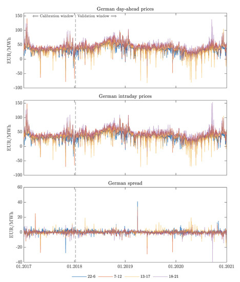
Figure 1.
German day-ahead prices (top panel), intraday prices (middle panel) and the spread, i.e., the difference between day-ahead and intraday prices (bottom panel). For illustration the hourly prices were averaged over four representatives blocks of hours: 22–6 (night), 7–12 (morning peak), 13–17 (midday), 18–21 (evening peak). Source: Authors’ elaboration.
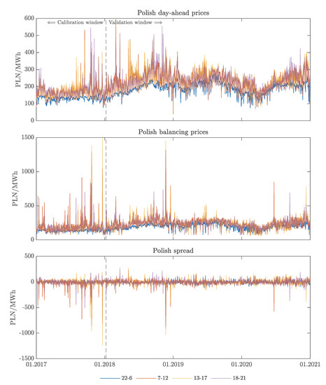
Figure 2.
Polish day-ahead prices (top panel), balancing prices (middle panel) and the spread, i.e., the difference between day-ahead and balancing prices (bottom panel). For illustration the hourly prices were averaged over four representatives blocks of hours: 22–6 (night), 7–12 (morning peak), 13–17 (midday), 18–21 (evening peak). Source: Authors’ elaboration.
For the German markets, the day-ahead and intraday prices contain many negative values, which are observed frequently in the morning and afternoon hours. On the other hand, high prices are observed mostly during the morning and evening peaks. Prices are also more volatile at the end of year, with an exception for 2020. These observations can be explained mostly by the high RES share in the German market and the impact of COVID-19 pandemic in year 2020. Pandemic caused a decrease in demand and this visibly induced the smaller prices. The spread presented in the bottom panel of Figure 1 shows that, although the day-ahead and the intraday prices have similar characteristics, the difference between them can be significant.
The Polish market has a significantly smaller share of RES. As for 2021, the share of RES for Germany was approximately 50% and for Poland only 15% [1]. Although the number and capacity of RES generators in Poland increases, it is still a very different market than in Germany, what yields different characteristics of electricity prices. Indeed, there are no negative prices in the Polish market. Instead, high positive price spikes are frequently observed, especially during the day. In the night hours rather price drops occur but their magnitude is much lower than in the German market. The difference between balancing and day-ahead markets is more pronounced. The balancing prices are more volatile and spiky. Only during the night hours prices behave similarly to the day-ahead prices from the same block.
3. Models
There are many modeling techniques that were used for short-term electricity price forecasting, like among others, statistical (see, e.g., [29,30,31]) or machine learning (see e.g., [26,32]) approaches. See also [33] or [34] for comprehensive reviews. Here, we follow [8,9,10] and use econometric approach based on time series models.
3.1. The Mean Model
As the mean model for electricity prices from both markets we use Autoregressive model with eXogenous variables (ARX), which is a standard approach in electricity price modeling. In the ARX model, electricity prices are explained by a linear relation with technical, business and market variables. Although the model is quite simple, many authors have shown its good performance, as compared to more sophisticated nonlinear methods, especially in a short-time horizon (see [33] and references therein). Precisely, the considered hourly day-ahead prices are modeled as 24 one-dimensional time series of the form
where h is the given hour and t denotes time in days, while is the stochastic noise. Similarly, the complementary (i.e., intraday or balancing) market prices, , are given by
The vector consists of dummy variables, which account for varying business conditions within a week. Here, the distinction is made between Monday, Saturday, Sunday/Holiday, and the other days of the week. Such vector reflects the weekly seasonality of electricity prices. Further, is a vector of exogenous variables. In this paper, we consider a set of all exogenous variables from Table 1. The weekly seasonality, being a typical property of electricity markets, is reflected in 7-daily lags of the autoregressive part in (1) and (2). Since a decision regarding the trade on the day-ahead market must be done before closing of the corresponding auction and not all complementary market prices on day are already known, we exclude lag 1 from the autoregressive part in the complementary market model, (2). Instead, following [8], the day-ahead price from day , , is included in the model for the complementary market prices, (2). Finally, the intraday effects are taken into account by considering the maximal and minimal prices from the previous day with known prices, and . Note, that following [10], for the German data and the intraday market model (2), the minimum and maximum prices for day t are replaced by the minimum and maximum of the day-ahead prices from day . After such change, the model yielded better results in terms of forecasts. The German intraday auction-based market is closed only three hours after the day-ahead auction, so the day-ahead prices have similar characteristics to the intraday prices.
3.2. The Variance Models
ARX model is based on the assumption that the volatility of the error term is constant over time. This seems to be justified, if only point forecasts are the objective of the analysis. However, when considering probabilistic forecasts, allowing for the model heterogeneity might bring significant improvement, see e.g., [21]. This is particularly important, if volatility based risk forecasts are the principle in a decision making process. We assume that the error terms for both markets and are given by the General Autoregressive Conditionally Heteroscedastic (GARCH) model, [16], i.e.,
where are zero-mean, finite-variance, i.i.d. random variables, , and are the model coefficients, while are the conditional variances. The model specification (3) allows for time dependence in the volatility of the error term, with the current variance being the function of the previous variance and the square of the previous error term. Note, that here we use only lags of order 1, i.e., GARCH(1,1) model. Based on a time analysis of autocorrelation (ACF) and partial autocorrelation (PACF) values it seems to be enough for capturing heteroscedasticity of prices and not overparametrizing the model. A similar choice was done e.g., by the authors of [17,19].
The GARCH model specification (3) yields a symmetric relation between the current volatility and the past values of the error terms, neglecting their sign. Since electricity prices considered in this paper are not symmetric and the market differently responds to negative and positive shocks (see Figure 1 and Figure 2), we also consider an asymmetric generalization of the GARCH model, namely the GJRGARCH [35]
where are zero-mean, finite-variance, i.i.d. random variables, , , and are the model coefficients, is the indicator function, while are the conditional variances. Note that for , the GJRGARCH model simplifies to the GARCH model, while for and the resulting volatility is constant, yielding a simple ARX model, (1) and (2).
The GARCH (or GJRGARCH) model is applied to the volatility of the ARX model errors, yielding an ARX-GARCH (ARX-GJRGARCH) model for the prices. For simplicity of the notation, we will further denote it just as the GARCH (or GJRGARCH) model.
3.3. Variance Stabilizing Transformation
For the considered markets, both day-ahead and complementary prices exhibit high volatility and price spikes. According to [36], lower variation of data usually leads to more accurate predictions. Therefore, following [37], we apply a mean normalization and an area hyperbolic sine (asinh) variance stabilizing transformation to the prices. It leads to dampening of both downward and upward spikes and symmetrizes the prices. This transformation can be viewed as a substitute of the log-transform that is not feasible for most electricity markets due to occurrences of negative prices. Adding a constant to the prices might allow for logarithmic transformation, but this would be problematic in practice. While finding such a constant in-sample is possible, we do not know if the future price would always be greater. Moreover, such an approach cannot be used for dampening of downward spikes, as those would be enlarged instead. Asinh transformation is therefore a relatively simple alternative that has logarithmic tail behavior for both positive and negative values (see [37] for a discussion on transformations for electricity prices).
Let us define the normalized price as
where b is the standard deviation of in the calibration window and a is the mean of this sample. Asinh transformation is then given by the formula
where is the normalized price from Equation (5) and the second equality comes directly from the definition of the area hyperbolic sine (asinh) function. Further, if the transformation is used, the Models (1)–(4) are applied to the transformed prices . The plots of transformed prices are given in the Appendix A (see Figure A1 and Figure A2).
Overall, we use six modeling approaches: (i) ARX model with a constant variance applied to prices (denoted by ARX); (ii) ARX model with a constant variance applied to transformed prices (denoted by ARX asinh); (iii) ARX-GARCH(1,1) model applied to prices (denoted by GARCH); (iv) ARX-GARCH(1,1) model applied to transformed prices (denoted by GARCH asinh); (v) ARX-GJRGARCH(1,1) model applied to prices (denoted by GJRGARCH); (vi) ARX-GJRGARCH(1,1) model applied to transformed prices (denoted by GJRGARCH asinh).
3.4. Model in-Sample Evaluation
Before deriving the price forecasts we briefly evaluate the in-sample fit of the models. The study uses a rolling window scheme. The coefficients of the ARX models, (1) and (2) are estimated in a calibration window using the least squares method separately for each hour h. The calibration window is then shifted one day forward and the procedure is repeated. We evaluate the fit of the model for each calibration window. The length of the calibration windows is set to 365 days, i.e., one year. The first calibration window is marked in Figure 1 and Figure 2 with a vertical line. In total we have 1088 calibration windows. Note that the last price in the calibration window is not known yet for complementary markets, so Equation (2) is estimated based on widow .
We start with verifying the presence of possible heteroscedasticity in the series of the ARX model residuals , using the ARCH–LM test by [38]. Precisely, we use the procedure suggested by [39] to account for a possible misspecification of the conditional mean, which might lead to over-rejection of the null hypothesis of homoskedasticity (see [40]). Technical details of the procedure are given in the Appendix. The obtained results are presented in Table 2. The hypothesis of no ARCH effects in residual series was rejected in of the calibration windows, depending on the market and weather data were transformed. The evidence is in general more pronounced if the asinh transformation is applied prior to the model estimation, especially for the Polish balancing and German intraday markets. For the Polish day-ahead market we get a different picture. Here, the significant ARCH effects are detected in more windows if the model is applied to nontransformed prices.
Table 2.
Percentage of rejected hypotheses in tests for residuals on: (i) no ARCH effects; (ii) Gaussian distribution; (iii) Student’s t distribution. All tests were performed on a significance level. For transformation denoted by ‘—’, the models were fitted to nontransformed prices.
The procedure of applying GARCH(1, 1) in the rolling window is straightforward. In each step we fit the model to in-sample residuals obtained from the ARX model given by Equations (1) and (2). We use the maximum likelihood method to estimate the model coefficients. It requires assuming the distribution of , (see (3) and (4)). Here, we use the Gaussian and Student’s t distributions. The choice is further evaluated based on the Kolmogorov–Smirnov goodness of fit test applied for the sample of standardized residuals, i.e., , , where is the estimated GARCH volatility. The obtained results are given in Table 2. Again, asinh transformation usually improves the fit. For the German markets Gaussianity is rejected only in 2–3% of 1088 calibration windows, which is below the significance level. For the Polish markets, an acceptable fit is obtained only for the Student’s t distribution. Hence, further for the estimation of the GARCH model, we assume a Gaussian distribution for the German markets and Student’s t for the Polish ones.
4. Price Forecasts
A proper planing of operational decisions of an electricity market participant requires a knowledge about possible future price movements. If profit is the only objective, then decisions can be made based on the point forecasts. However, if also a risk and uncertainty mitigation is the aim, then a knowledge about predicted price distribution is important. In this section we first introduce and briefly evaluate point forecasts obtained for the considered models. Next, we compare the accuracy of the corresponding probabilistic forecasts.
4.1. Point Forecasts
If the variance stabilizing transformation is not applied, the point forecasts of the prices are simply given by a linear combination of the explanatory variables with the parameters estimated from a preceding calibration window. The situation is different, if the asinh transformation is used and the model is fitted to the transformed prices, . Then, the forecasts can be simply derived for transformed prices, , but the backward transformation is not straightforward, due to non linearity of the asinh function (see [41] for a discussion on this issue). Here we use the mathematically correct approach and approximate the point forecasts of prices as the mean of simulated scenarios of transformed prices:
where each scenario , is simulated from the fitted ARX or GARCH model and are the parameters used for normalization in (5). The transformed price scenarios are calculated using the historical simulation method, i.e., , where are either the in-sample residuals from the ARX model or the in-sample standardized residuals multiplied by the forecasted volatility for the GARCH model. In the case of complementary market, a two-step GARCH forecast is used, analogously as lags in (2).
We evaluate the performance of the point forecasts using the Mean Absolute Error (MAE) calculated for each hour in the validation window separately , with . The results obtained for the ARX model for each hour as well as their hourly average are given in Table 3. The values of MAE for the GARCH and GJRGARCH models are not reported in the table, as they are not significantly different from the ones obtained from the ARX model, according to the one-sided Diebold–Mariano test on equal predictive accuracy [42]. Here, the accuracy of the point forecasts is driven by the mean model, described by the ARX equation in all cases.
Table 3.
Mean absolute error (MAE) of hourly point forecasts obtained from the ARX model fitted to prices as well as prices transformed using asinh function. The unit of MAE is EUR/MWh and PLN/MWh for Germany and Poland, respectively. For each market, each hour as well as their hourly average (last row) significantly lower values according to the Diebold–Mariano test calculated at significance level are denoted by *.
According to the values of MAE, the variance stabilizing transformation (asinh) yields a significant difference in the forecast accuracy. For both German markets and the Polish balancing market, applying transformation prior to the model estimation leads to improvement of the forecast accuracy for most hours. This effect is especially apparent during the day, namely 12–20 h for the German markets and 7–21 h for the Polish balancing market, when the prices are usually higher and more volatile. For the Polish day-ahead market transformation applied to prices prior to the model estimation leads to significantly lower accuracy of the point forecasts for 12 of the hours and an improvement only for the evening peak at 20 h. The average of hourly MAE for the Polish day-ahead market is higher if transformation is applied. However, according to the Diebold–Mariano test, this difference is not significant at the significance level.
4.2. Probabilistic Forecasts
One can use several methods (see [43] for a review on probabilistic forecasting for electricity prices) to derive the possible scenarios of the next-day price. In the paper we use the historical simulation [44] and generate a sample of possible price scenarios for the next day using the sample of bidimensional model residuals from the calibration window. The predicted distribution is then approximated by the empirical distribution of the simulated samples. Precisely, the jth price scenario for the hth hour on day is calculated as
If no transformation is used or
If the case of the asinh transformation. Variables are either the in-sample errors of the fitted ARX model or, for the GARCH (GJRGARCH) model, , where is the forecasted volatility based on (3) (or (4) for GJRGARCH) and are the standardized in-sample residuals. N is the length of the calibration window i.e., . Finally, for the Polish balancing market we impose price caps of on the simulated scenarios, in compliance with the market regulations.
The probabilistic forecasts are evaluated in the validation window using the Pinball loss function (PL) [45]
where is the qth quantile of the forecasted price distribution and is the actually observed value. Note that can be calculated for each hour h and day t in the validation window and a chosen qth quantile. Here, we evaluate the fit in all percentiles, i.e., . The pinball values are then averaged over all quantiles for a given hour, producing an hourly pinball score, or over all hours for a given quantile, yielding a percentile pinball score. The mean scores obtained in the validation window for the considered models and both markets are plotted in Figure 3 and Figure 4. In all cases except for the Polish day-ahead market a significant improvement in the fit of probabilistic forecasts can be observed if the asinh transformation is applied prior to the model estimation. The highest difference between the pinball scores obtained for models with or without transformation is obtained for the midday, i.e., 10–18 h for the German markets and 8–21 h for the Polish balancing market. It is also observed for the middle range of the quantiles with a small shift towards quantiles lower than median for the German market and higher than median for the Polish balancing market. Recall, that the German prices are characterized by large drops, while the Polish prices by spikes. These observations are more affected by the transformation, yielding larger differences from the forecasts obtained without transformation. For the Polish day-ahead market, the influence of the transformation is not that clear. It yields lower values of the mean pinball score for the noon (10–12) and evening peaks (18–20) and higher for the afternoon peak (14–16).
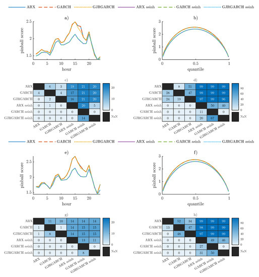
Figure 3.
Pinball scores obtained for probabilistic forecasts of the German day-ahead (panels (a–d)) or intraday (panels (e–h)) electricity prices obtained using ARX, GARCH and GJRGARCH models with or without asinh transformation. The mean score over all percentiles for each hours is plotted in the left panels ((a)—for day-ahead and (e)—for intraday), while the mean over hours for each quantile in the right panels ((b)—for day-ahead and (f)—for intraday). The corresponding, aggregated, one-sided Diebold–Mariano test results are given in the corresponding bottom panels (c,d,g,h). Source: Authors’ elaboration.
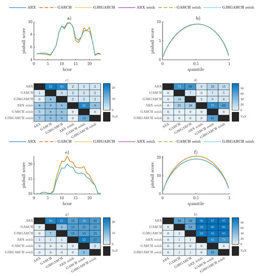
Figure 4.
Pinball scores obtained for probabilistic forecasts of the Polish day-ahead (panels (a–d)) or balancing (panels (e–h)) electricity prices using ARX, GARCH and GJRGARCH models with or without asinh transformation. The mean score over all percentiles for each hour is plotted in the left panels ((a)—for day-ahead and (e)—for balancing), while the mean over hours for each quantile in the right panels ((b)—for day-ahead and (f)—for balancing). The corresponding, aggregated, one-sided Diebold–Mariano test results are given in the corresponding bottom panels (c,d,g,h). Source: Authors’ elaboration.
The significance of the differences between the models is further evaluated pairwise using the one-sided Diebold–Mariano test. The obtained results for each pair of the considered models are plotted in Figure 3 and Figure 4. Precisely, we calculate the number of hours (left panels) or percentiles (right panels) for which the test hypothesis that the model in a given row is not worse than the model in a given column, was rejected at the significance level. For both German markets and the Polish balancing market the asinh transformation significantly improves the results for most hours and percentiles and all of the considered models. For the Polish day-ahead market the accuracy of the probabilistic forecasts is overall slightly lower if transformation is applied. Comparing the fit of the ARX, GARCH and GJRGARCH models, we can observe a significant improvement if time-varying volatility is taken into account. The GARCH and GJRGARCH models outperform the ARX model for all markets and both approaches to transformation, except only for the percentile pinball scores for the day-ahead German market and no transformation. Except for the Polish day-ahead market, the difference between the GARCH and the ARX models is even strengthen if transformation is applied. Then in all cases, the GARCH model yield significantly more accurate probabilistic forecasts then ARX. Such effect is not visible for the GJRGARCH model, which is always outperformed by the GARCH model for transformed prices, while in the case of no transformation the overall fit is comparable.
The GARCH model significantly improves the accuracy of probabilistic forecasts, so it will be further used for a strategy construction. On the other hand, the asinh transformation significantly improves the probabilistic as well as point forecasts for both German markets and the Polish balancing market. Hence, further we will use transformed prices for these three markets and nontransformed prices for the Polish day-ahead market.
5. Portfolio Selection Based on Probabilistic Forecasts
We assume that an electricity trader (buyer or seller) can decide on the day preceding delivery on the percentage of energy to be sold (for seller) or bought (for buyer) on the day-ahead market. The remaining part is then sold (or bought) on the complementary market, i.e., intraday for Germany or balancing for Poland. Additionally, we assume that the trader is a price taker, so his decisions do not influence the auction results and that the volume of the trade is constant. In the following we propose different strategies for the choice of the market, aiming at risk minimization, profit maximization or an optimal trade-off between these two.
5.1. Strategies
Using the day-ahead probabilistic forecasts of the prices from the day-ahead and complementary markets, (8) and (9), we can simulate possible scenarios of the next day price composed of energy sold (bought) on both markets as
where is a part of energy sold on the complementary market, while , is the price scenario for the complementary and the day-ahead market, respectively. In order to recover the joint distribution, the residuals from both markets used for scenario generation are treated as a bidimensional sample. Because the calibration window for complementary market does not contain the current day price, the corresponding residuum from the day ahead sample is not taken into account in scenario generation. Given a vector of simulated scenarios, , different risk and profit measures can be calculated for both, a seller and a buyer of energy. Strategies for a buyer can be constructed using the same algorithms as for a seller, but applied to prices with a negative sign. It comes from the fact that minimizing the price is equivalent to maximizing its negative value, i.e., and a buyer, contrariwise to a seller, would minimize the price he has to pay for energy. For clarity, we give also the buyer’s objectives explicitly.
We use three strategies that are focused only on the risk minimisation. Those are represented by the standard deviation (volatility, std) and semistandard deviations (sstd), measuring only up or downward risk. Due to its symmetry, std is the same for a buyer and a seller and so the strategy for both positions is based on
where is the standard deviation of the portfolio price scenarios, see Equation (11).
The standard deviation as a risk measure in its classic form treats all deviations from the mean as risky. However, depending on the trader’s position, the risk is not the same for high and low prices. Hence, the second risk-minimizing strategy is based on the semistandard deviation (sstd). For a seller we use sstd that takes into account only prices that are below the mean, i.e., cause losses with respect to the average price. The optimization problem is then given by
On the other hand, for a buyer we use sstd, which calculates deviation of the prices that are higher than the expected value, i.e., are more expensive than the average price. The optimization problem is then given by
We also consider three strategies aimed at finding the optimal trade-off between the risk and return. Those are further called the optimal strategies. The first one is based on minimization of risk, given that the return of strategy is greater than return from trading only on the day-ahead market. This is assured by an additional condition in the optimization problem. For a seller it is given by
While for a buyer
We further call this strategy ’std-profit’.
A second optimal strategy is based on the Sharpe ratio [46] idea, which in the classical form is defined as the profit over the risk-free rate per unit of risk. Here, the risk is measured by the standard deviation and the profit as the expected value of the diversified price (11). If the seller’s position is analyzed and the profits are positive, then maximization of the Sharpe ratio leads to maximization of profit and, at the same time, minimization of risk. However, electricity prices can be negative. In such a case maximum Sharpe ratio would be achieved for a maximized value of risk. Hence, we propose to use the following modification of the Sharpe ratio
On the other hand, if a buyer’s perspective is taken into account, the objective is to minimize the expected price together with minimizing the risk. For a positive price this can be achieved by minimizing the product of the expected value and standard deviation. For negative prices, analogously as for a seller, the product needs to be replaced with a fraction, i.e., we have
The last optimal strategy considered in this work maximizes profit under the assumption, that the volatility of diversified price, (11), is not greater than the volatilities of both markets. Hence, the optimization problem for a seller is given by
while for a buyer by
We further call this strategy ‘mean-std’. In contrast to ‘std-profit’ strategy, here, the objective is the profit maximization with a risk control.
Finally, we also use a strategy based only on the profit maximization. For a seller the optimization problem is given by
while for a buyer by
Note that, since the expected portfolio price is a linear combination of the expected prices from both markets, the profit maximization strategy will simply aim at choosing the market with a higher expected price, i.e., will yield . We further denote this strategy by ‘mean’.
All of the above objectives are based on the first and second moments of the diversified price (11) distribution. Since this price is a linear combination of prices from both markets, each of the objectives can be rewritten in terms of a polynomial function of weight with parameters given by the moments of the forecasted distributions of prices from both markets and the covariance of their joint distribution as well as the corresponding semi second moments in the case of sstd. Once these parameters are given, some of the problems, like the volatility minimization or profit maximization can be solved analytically. However, since this cannot be done in general, for unification in the practical application we search for the optimal weights numerically in all cases.
5.2. Evaluation of the Obtained Portfolios
We apply each of the proposed strategies in the rolling window scheme, i.e., for each day t and hour h in the validation window we calculate day-ahead probabilistic forecasts of prices from both markets using the ARX-GARCH model (see Section 4.2 for details). Based on the results of Section 3.4 and Section 4 we apply the variance stabilizing asinh transformation prior to the model estimation for prices from both German markets and the Polish balancing market. The predicted distribution is then used in the optimization problem to derive the percentage of energy to be sold (for seller) or bought (for buyer) on the day-ahead market, based on a given objective of the strategy. In this way a decision is made separately for each hour and day, so it dynamically adjusts to changing market conditions. The strategy outcome is then evaluated in the whole validation window.
Having the forecasts of mean, variance, and covariance of the prices as well as their semianalogs, the optimization problems specified in Section 5.1 can be treated as linear or quadratic programming problems with constraints (see e.g., [47] for a review on mean–variance optimization problems). To solve them, we apply the interior-point algorithm as this flexible method has proven to perform well on both large and small scale problems [48]. We use a Matlab fmincon function with a starting solution that is found based on a grid search over ten equally spaced weights from range .
We start with calculating mean of the energy price, (11), obtained for each of the strategies. We also calculate the corresponding standard deviation of the prices. The results for each hour and both, buyer and seller, are given in Figure 5 and Figure 6, for Germany and Poland respectively. For the German markets there are small differences between mean day-ahead and intraday prices, so the mean strategy price is also close to these prices. Larger differences are observed in the standard deviation, especially during the evening peak, with more volatile intraday prices. Strategies aimed at profit maximization yield mean prices that are close to the prices of the market with higher (for a seller) or lower (for a buyer) prices. Interestingly, it leads to a higher standard deviation for a buyer, especially in the evening peak and during the night, when more price drops are observed. On the other hand, strategies with an objective in risk minimization lead to lowering the standard deviation in all cases.
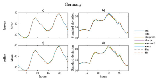
Figure 5.
Means (for buyer—panel (a) and for seller—panel (c)) as well as standard deviations (for buyer—panel (b) and for seller—panel (d)) of hourly prices in the validation window obtained from different strategies in the German market. For reference, also the results of trading only on the day-ahead (DA) or intraday (ID) market are plotted with dashed lines.Source: Authors’ elaboration.
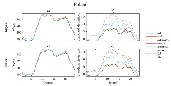
Figure 6.
Means (for buyer—panel (a) and for seller—panel (c)) as well as standard deviations (for buyer—panel (b) and for seller—panel (d)) of hourly prices in the validation window obtained from different strategies in the Polish market. For reference, also the results of trading only on the day-ahead (DA) or balancing (BL) market are plotted with dashed lines. Source: Authors’ elaboration.
For Poland the differences between the markets are more pronounced. The balancing market is characterized by higher average prices than the day-ahead market and at the same time much higher volatility. Here, price maximization leads a seller to trading mostly on the balancing market, but especially during the afternoon even a higher prices can be achieved by combining it with a day-ahead market trading. On the other hand, a buyer strategy with an objective in price minimization leads to trading mostly on the day-ahead market, but again even lower prices can be achieved, if using a strategy. For strategies aimed at profit maximization, a higher volatility is related to selling, what is a consequence of price spikes, characterizing the balancing market. This is not the case, if risk is also controlled in the strategy. Then for both, a buyer and a seller, most trade is done on the day-ahead market. Overall a buyer would mainly trade on the day-ahead market with lower prices and lower volatility. For a seller a choice is dependent on the general objective, as profits are higher on the balancing market, but at the cost of higher volatility.
Looking at Figure 5 and Figure 6a clear hourly pattern can be observed with significant differences between times of the day. Hence, we further analyze results separately for four blocks of hours: (i) night (22 h–7 h) with the lowest prices and volatility; (ii) morning peak (8 h–12 h) with high prices and volatility; (iii) afternoon (13 h–17 h) with moderate prices and volatility; (iv) evening peak (18h–21h) with high prices and volatility. In Figure 7, Figure 8, Figure 9 and Figure 10 we plot the mean prices versus the standard deviation for each of the strategies averaged over a given block of hours. For reference we also plot the corresponding values for both markets. These would be the outcomes of trading only in one of the markets with no strategy used.
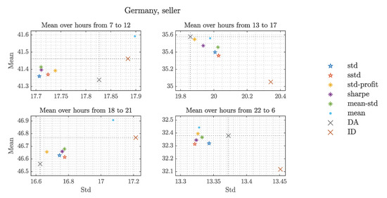
Figure 7.
Average results of the portfolio allocation, obtained for a seller in the German market using different strategies. The averages are calculated over all days in the validation window and hours within the considered blocks: 7–12, 13–17, 18–21, 22–6. The results of trading only on the day-ahead (DA) or intraday (ID) market are plotted for reference. Source: Authors’ elaboration.
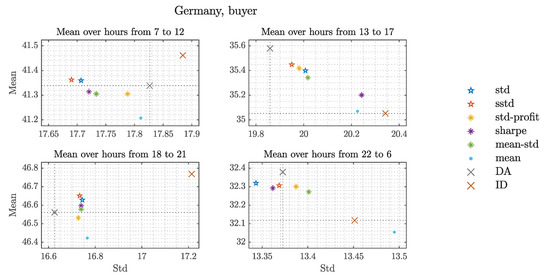
Figure 8.
Average results of the portfolio allocation, obtained for a buyer in the German market using different strategies. The averages are calculated over all days in the validation window and hours within the considered blocks: 7–12, 13–17, 18–21, 22–6. The results of trading only on the day-ahead (DA) or intraday (ID) market are plotted for reference. Source: Authors’ elaboration.
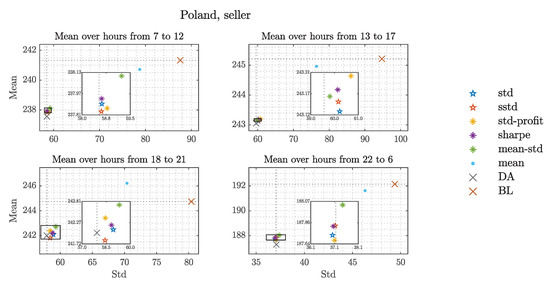
Figure 9.
Average results of the portfolio allocation, obtained for a seller in the Polish market using different strategies. The averages are calculated over all days in the validation window and hours within the considered blocks: 7–12, 13–17, 18–21, 22–6. The results of trading only on the day-ahead (DA) or balancing (BL) market are plotted for reference. To improve visibility, a zoom from the area marked with rectangles is also plotted. Source: Authors’ elaboration.
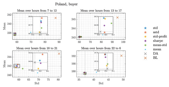
Figure 10.
Average results of the portfolio allocation, obtained for a buyer in the Polish market using different strategies. The averages are calculated over all days in the validation window and hours within the considered blocks: 7–12, 13–17, 18–21, 22–6. The results of trading only on the day-ahead (DA) or balancing (BL) market are plotted as for reference. To improve visibility, a zoom from the area marked with rectangles is also plotted. Source: Authors’ elaboration.
For the German market the strategy aiming only on the profit maximization yields profits that are not only higher than obtained from the other strategies, but also higher than the means from both markets. Usually it is achieved at the cost of higher standard deviation. Controlling risk lowers the standard deviation in most cases, but the profits are also lower. Comparing different blocks of hours, the best results were obtained for the morning peak with lower standard deviation and, especially for a buyer, higher profit than from both markets, if it is controlled in a strategy. For both, afternoon and evening blocks, the outcomes of the strategies with a risk control are between both markets. During the night the risk is lowered as compared to both markets, if it is taken into account. For a seller the optimal strategies ‘std-profit’ and ‘mean-std’ yield better result than each of the markets, both in the mean and standard deviation.
Results of the strategies obtained for the Polish market are on average similar for all blocks of hours. If risk is taken into account, then most of the trade is done on the day-ahead market. If a higher profit is the objective, then more energy is traded on the balancing market. This effect is more pronounced for a seller, which benefits from price spikes.
The comparison with trading only on the day-ahead and complementary markets is further evaluated in Table 4. We calculate an overall profit of the strategies with respect to trading only on one of the markets. For a seller it is given by
where i denotes the reference market and T is the length of the validation window. For a buyer the profit is given by
Table 4.
Strategy results in the validation window for different objectives for the Polish and German market: total profit over trading only on one of the markets (p-DA for the day-ahead, p-BL for the balancing and p-ID for the intraday market) as well as the portfolio standard deviations (std).
In Table 4 we also present the average of the hourly standard deviations of the prices resulting from the strategies, (11). The corresponding standard deviations of prices are equal to 16.39 for the German day-ahead market, 16.59 for the German intraday market, 50.61 for the Polish day-ahead market and 73.57 for the Polish balancing market.
Strategies aiming at risk minimization, indeed yield lower average standard deviations. Usually risk mitigation is achieved at the cost of lower profits. However, applying additional condition on the expected prices (strategy ’std-profit’) yields the lowest risk for a seller on the German market and buyer on the Polish market with one of the highest profits. For the German market the best results in terms of profits were achieved with the ’mean’ strategy, but dropping the risk control visibly increases standard deviation (see Table 4). Interestingly, for a buyer on the Polish market better results, not only in risk but also in profit, were achieved by the ’std-profit’ and ’mean-std’ strategies. For a seller in the Polish market, a significant difference between the ’mean’ strategy and strategies that include risk control can be observed. A seller that aims at profit maximization would trade mostly on the balancing market, which on average has much higher prices than the day-ahead market. On the other hand these prices are also much more volatile than the day-ahead, so all strategies that involve risk measure in the objective function would yield much higher weights for the day-ahead market.
Finally, we compare the overall performance of the strategies by calculating the mean diversified price per unit of risk. This ratio might be interpreted as a measure of the final risk–return trade-off. The price is averaged over all hours and days in the validation window, while the risk is measured by the corresponding, averaged standard deviation. The values for both markets and all strategies are given in Table 5. In order to reflect the opposite positions of seller and buyer, the latter’s price is multiplied by . As a consequence for both positions higher ratio means a better risk–return trade-off. The obtained results indicate that for the seller’s strategies best results are achieved if risk is taken into account. Especially, for the Polish market, the simple profit maximization strategy yields much lower ratio. The highest values are obtained for the strategies that are based on both, risk and profit, objectives. However, the differences with simple risk minimization strategies are not high. On the other hand, for the buyer’s perspective the profit maximization strategy yields the best results. Again the difference is more pronounced for the Polish market. Buyer in the German market benefits from price drops, so reducing the standard deviation caused mainly by downward spikes is not his objective. In the case of the Polish market, buyer would mainly trade in the day-ahead market, which is represented by lower prices and lower standard deviation. Hence, profit maximization would also lead to lowering risk.
Table 5.
The average price of a seller as well as a buyer per unit of risk, measured by a standard deviation. The buyer’s prices are negative to denoted the outflow, while the seller’s positive to denote the inflow.
6. Summary and Discussion
In this paper, we have generalized approach of [10] by considering the GARCH model for volatility forecasts of the day-ahead and complementary (intraday or balancing) markets in Germany and Poland. By including interrelations between the markets in the ARX equations as well as bivariate distribution of the GARCH residuals we used a joint heteroscedastic model for the day-ahead and complementary markets. We have shown that including a time-varying, heteroscedastic volatility improves probabilistic forecasts (except for the Polish day-ahead market), especially if a variance stabilizing transformation is applied prior to the model estimation. While it is widely agreed that using a variance stabilizing transformation is important for fitting linear models to electricity prices, we show that it is also important, when modeling heteroscedastic effects by the GARCH model. However, we have found that the transformation is not always optimal. For the Polish day-ahead prices considered in this paper, applying the variance stabilizing transformation worsen the in-sample fit as well as the forecasting performance. Hence, we believe that the effects of variance stabilizing transformation on electricity prices should be always verified for considered datasets before the final choice of the modeling approach.
The price forecasts were used as a basis for constructing dynamic, day-ahead diversification strategies. In contrast to the previous studies, we considered not only seller’s but also buyer’s perspective. We proposed several objectives using the forecasted volatility aiming at the risk minimization and/or profit maximization. The objectives were based on the mean–variance portfolio theory. However, we have adjusted some of the measures for electricity prices. In particular, we use a semistandard deviation, which in contrast to the standard deviation is not symmetric around mean, and hence involves different perspectives of a buyer and seller. We have also modified the classical Sharpe ratio objective to account for negative prices and the buyer’s position. We evaluated the outcomes of the proposed strategies in three-yearly validation window for the markets in Germany and Poland. We found that strategies designed for risk mitigation, indeed, yielded the lowest volatilities, but at the cost of low profits. On the other hand, if the profit was the only objective, the risk has significantly increased. Strategies combining both, profit maximization and risk minimization, lead to a risk–return balanced results.
We applied the proposed approach for two electricity markets with significant differences in price characteristics. First, the Polish market experiences high price spikes, whereas German prices are characterized by downward spikes that include negative prices. Second, the prices from the Polish balancing market are on average higher than the day-ahead prices, but this is accompanied by much higher standard deviation. For the German market the differences between day-ahead and intraday prices are lower and rather symmetric. Surprisingly, if a single-value comparison between strategies, representing the risk–return trade-off, is made, the results for both markets yield to similar conclusions. For the seller’s strategies best results are achieved, if risk is taken into account. On the other hand, for the buyer’s perspective the pure profit maximization strategy yields the best results. However, if we also look on the comparison with pure day-ahead or complementary market trading a clear difference between the countries can be observed. In the case of the Polish market, if risk mitigation is taken into account, then most of the trade should be done in the day-ahead market. If a higher profit is the objective, then more energy should be traded in the balancing market. This effect is more pronounced for a seller, which benefits from price spikes. For the German market risk mitigation strategies might be beneficial from the seller’s perspective with both, risk and profit, improved as compared to trading only in one of the markets. Using risk minimization as the objective for the German market results in avoiding drops in prices, what is profitable for sellers. On the other hand, for a buyer risk mitigation strategies yield lower profits than trading purely in the intraday market.
The presented approach can be further improved. First, the volume risk was not taken into account. For an electricity trader it would require an analysis of individual production or demand size. While the price risk is common for all market participants, the volume risk, especially from RES production, is varying between the traders, see e.g., [49,50] for different production profile analysis. If the forecasts of individual trading volume were known, then they could be simply incorporated into the price model, as the product of forecasted price and volume, see [51] for the SVAR model approach with an overall RES production forecasts or [52,53] for an analysis of the product distribution in the context of electricity markets. Second, in the paper, we have followed the approach of [8,9,10] and for comparability we used the ARX as the mean model. Using other models with a good predictive performance for electricity prices, like e.g., LASSO, [30], might improve strategy outcomes. Third, we assumed that the trader is a price taker, neglecting the influence of trading decisions on auction results. The authors of [10] showed how diversification strategies can be approximately adjusted using a scaling parameter that reflects the size of the trader’s influence. A more accurate approach would require an analysis of bid/ask and supply/demand curves, see e.g., [54,55,56] for an application of such approach. Finally, when finding optimal weights we assumed that the parameters of the forecasted distribution can be calculated exactly. This assumption was validated in the final analysis of the strategy outcomes. However, estimation of parameters from a finite sample is burdened with uncertainty and as a consequence a possible bias. One of the possible solutions is to improve the estimation procedure, using e.g., the bootstrap method. Another possibility is to include uncertainties in the weights optimization procedure, using the so-called robust optimization (see e.g., [47] for a comprehensive review on this issue).
We believe that adjusting the presented general approach in an individual context would help electricity traders in finding an optimal risk–profit balance for a company. Since electricity is a special commodity with limited storage possibilities and extreme price volatility, standard risk management strategies, that are well developed for other commodities or financial markets cannot be easily adopted. Instead, a short-term, operational planning of wholesale electricity trade can be dynamically optimized. We believe that the proposed diversification strategies might be utilizied in such practical context. Moreover, as the presented approach is fully automatic, it might improve a decision making process in operational time.
Author Contributions
Conceptualization, J.J.; methodology, J.J. and A.P..; software, A.P.; validation, J.J. and A.P.; formal analysis, J.J.; investigation, J.J. and A.P.; data curation, A.P.; writing—original draft preparation, J.J. and A.P.; writing—review and editing, J.J. and A.P.; visualization, A.P.; supervision, J.J.; project administration, J.J.; funding acquisition, J.J. All authors have read and agreed to the published version of the manuscript.
Funding
The research was financed by NCN Sonata grant No. 2019/35/D/HS4/00369.
Data Availability Statement
The German intraday market data is available from the EPEX SPOT. Other datasets are freely available from their sources given in Table 1.
Conflicts of Interest
The authors declare no conflict of interest.
Appendix A. Additional Figures

Figure A1.
German day-ahead prices (top panel), intraday prices (middle panel) and the spread (bottom panel) after the asinh transformation. For illustration the hourly prices were averaged over four representatives blocks of hours: 22–6 (night), 7–12 (morning peak), 13–17 (midday), 18–21 (evening peak). Source: Authors’ elaboration.


Figure A2.
Polish day-ahead prices (top panel), balancing prices (middle panel) and the spread (bottom panel) after the asinh transformation. For illustration the hourly prices were averaged over four representatives blocks of hours: 22–6 (night), 7–12 (morning peak), 13–17 (midday), 18–21 (evening peak). Source: Authors’ elaboration.

Appendix B. Misspecification Testing
The authors of [40] show, that the misspecification of the conditional mean over-rejects the null hypothesis for homoskedasticity. In our case, in-sample residuals from the ARX models defined in Equations (1) and (2) exhibit autocorrelation. We acknowledge the influence of such misspecification on the ARCH-LM test result and proceed to remove the autocorrelation from the residues following the procedure suggested by [39]. The method originally used by the authors was designed for the AR model, so we modify it slightly to fit the considered ARX model. The procedure is shortly described below.
Let us define the true model for the prices as
where we take to account for weekly seasonality and to include non-linear effects of exogenous variables, is an unknown function and is the vector of parameters. Let us assume that the disturbance term is given by Equation (3). We then assume that can be approximated by a sum of two functions: one of autoregressive and one of exogenous variables. Finally, we apply a 2nd-order Taylor approximation to the model from Equation (A1)
For German prices we include gas prices and CO emission prices only in the first order component. This decision is dictated by the fact that values of current and lagged gas prices and emissions were often the same, resulting in problems with the order of the parameter matrix used in the OLS estimation. The authors of [39] argue, that using residuals obtained from such polynomial approximation can be advantageous, since it is possible that they show size and power properties similar to those of the true model.
References
- Burger, B. Energy-Charts. 2022. Available online: https://www.energy-charts.info (accessed on 25 July 2022).
- Martinez-Anido, C.B.; Brinkman, G.; Hodge, B. The impact of wind power on electricity prices. Renew. Energy 2016, 94, 474–487. [Google Scholar] [CrossRef]
- Gianfreda, A.; Parisio, L.; Pelagatti, M. The impact of RES in the Italian day-ahead and balancing markets. Energy J. 2016, 37, 161–184. [Google Scholar] [CrossRef]
- Maciejowska, K. Assessing the impact of renewable energy sources on the electricity price level and variability—A quantile regression approach. Energy Econ. 2020, 85, 104532. [Google Scholar] [CrossRef]
- Kulakov, S.; Ziel, F. The impact of renewable energy forecasts on intraday electricity prices. Econ. Energy Environ. Policy 2021, 10. [Google Scholar] [CrossRef]
- Gholami, M.; Shahryari, O.; Rezaei, N.; Bevrani, H. Optimum storage sizing in a hybrid wind-battery energy system considering power fluctuation characteristics. J. Energy Storage 2022, 52, 104634. [Google Scholar] [CrossRef]
- de Siqueira, L.M.S.; Peng, W. Control strategy to smooth wind power output using battery energy storage system: A review. J. Energy Storage 2021, 35, 102252. [Google Scholar] [CrossRef]
- Maciejowska, K.; Nitka, W.; Weron, T. Day-ahead vs. intraday—Forecasting the price spread to maximize economic benefits. Energies 2019, 12, 631. [Google Scholar] [CrossRef]
- Janczura, J.; Michalak, A. Optimization of electric energy sales strategy based on probabilistic forecasts. Energies 2020, 13, 1045. [Google Scholar] [CrossRef]
- Janczura, J.; Wójcik, E. Dynamic short-term risk management strategies for the choice of electricity market based on probabilistic forecasts of profit and risk measures. The German and the Polish market case study. Energy Econ. 2022, 110, 106015. [Google Scholar] [CrossRef]
- Markowitz, H. Portfolio selection. J. Financ. 1952, 7, 77–91. [Google Scholar]
- Elton, E.J.; Gruber, M.J. Modern portfolio theory, 1950 to date. J. Bank. Financ. 1997, 21, 1743–1759. [Google Scholar] [CrossRef]
- Liu, M.; Wu, F.F. Risk management in a competitive electricity market. Int. J. Electr. Power Energy Syst. 2007, 29, 690–697. [Google Scholar] [CrossRef]
- Garcia, R.C.; González, V.; Contreras, J.; Custodio, J.E. Applying modern portfolio theory for a dynamic energy portfolio allocation in electricity markets. Electr. Power Syst. Res. 2017, 150, 11–23. [Google Scholar] [CrossRef]
- Roques, F.A.; Newbery, D.M.; Nuttall, W.J. Fuel mix diversification incentives in liberalized electricity markets: A Mean–Variance Portfolio theory approach. Energy Econ. 2008, 30, 1831–1849. [Google Scholar] [CrossRef]
- Bollerslev, T. Generalized autoregressive conditional heteroskedasticity. J. Econom. 1986, 31, 307–327. [Google Scholar] [CrossRef]
- Hickey, E.; Loomis, D.G.; Mohammadi, H. Forecasting hourly electricity prices using ARMAX–GARCH models: An application to MISO hubs. Energy Econ. 2012, 34, 307–315. [Google Scholar] [CrossRef]
- Garcia, R.; Contreras, J.; van Akkeren, M.; Garcia, J. A GARCH forecasting model to predict day-ahead electricity prices. IEEE Trans. Power Syst. 2005, 20, 867–874. [Google Scholar] [CrossRef]
- Tehrani, S.; Juan, J.; Caro, E. Electricity spot price modeling and forecasting in European markets. Energies 2022, 15, 5980. [Google Scholar] [CrossRef]
- Karakatsani, N.V.; Bunn, D.W. Fundamental and behavioural drivers of electricity price volatility. Stud. Nonlinear Dyn. Econom. 2010, 14. [Google Scholar] [CrossRef]
- Billé, A.G.; Gianfreda, A.; Del Grosso, F.; Ravazzolo, F. Forecasting electricity prices with expert, linear, and nonlinear models. Int. J. Forecast. 2022, in press. [Google Scholar] [CrossRef]
- Tan, H.; Li, Z.; Wang, Q.; Mohamed, M.A. A novel forecast scenario-based robust energy management method for integrated rural energy systems with greenhouses. Appl. Energy 2023, 330, 120343. [Google Scholar] [CrossRef]
- Chen, Z.; Jin, T.; Zheng, X.; Liu, Y.; Zhuang, Z.; Mohamed, M.A. An innovative method-based CEEMDAN–IGWO–GRU hybrid algorithm for short-term load forecasting. Electr. Eng. 2022, 104, 3137–3156. [Google Scholar] [CrossRef]
- European Energy Exchange. 2021. Available online: https://www.epexspot.com (accessed on 12 April 2021).
- Towarowa Giełda Energii. 2021. Available online: https://tge.pl/ (accessed on 12 April 2021).
- Lago, J.; Marcjasz, G.; De Schutter, B.; Weron, R. Forecasting day-ahead electricity prices: A review of state-of-the-art algorithms, best practices and an open-access benchmark. Appl. Energy 2021, 293, 116983. [Google Scholar] [CrossRef]
- Commission, T.E. Commission Regulation (EU) 2017/2195 of 23 November 2017 establishing a guideline on electricity balancing. Off. J. Eur. Union 2017, 312, 6–53. [Google Scholar]
- Polskie Sieci Energetyczne. 2021. Available online: http://www.pse.pl (accessed on 12 April 2021).
- Karakatsani, N.V.; Bunn, D.W. Forecasting electricity prices: The impact of fundamentals and time-varying coefficients. Int. J. Forecast. 2008, 24, 764–785. [Google Scholar] [CrossRef]
- Uniejewski, B.; Marcjasz, G.; Weron, R. Understanding intraday electricity markets: Variable selection and very short-term price forecasting using LASSO. Int. J. Forecast. 2019, 35, 1533–1547. [Google Scholar] [CrossRef]
- Kiesel, R.; Paraschiv, F. Econometric analysis of 15-minute intraday electricity prices. Energy Econ. 2017, 64, 77–90. [Google Scholar] [CrossRef]
- Luo, S.; Weng, Y. A two-stage supervised learning approach for electricity price forecasting by leveraging different data sources. Appl. Energy 2019, 242, 1497–1512. [Google Scholar] [CrossRef]
- Weron, R. Electricity price forecasting: A review of the state-of-the-art with a look into the future. Int. J. Forecast. 2014, 30, 1030–1081. [Google Scholar] [CrossRef]
- Petropoulos, F.; Apiletti, D.; Assimakopoulos, V.; Babai, M.Z.; Barrow, D.K.; Ben Taieb, S.; Bergmeir, C.; Bessa, R.J.; Bijak, J.; Boylan, J.E.; et al. Forecasting: Theory and practice. Int. J. Forecast. 2022, 38, 705–871. [Google Scholar] [CrossRef]
- Glosten, L.R.; Jagannathan, R.; Runkle, D.E. On the relation between the expected value and the volatility of the nominal excess return on stocks. J. Financ. 1993, 48, 1779–1801. [Google Scholar] [CrossRef]
- Janczura, J.; Trück, S.; Weron, R.; Wolff, R.C. Identifying spikes and seasonal components in electricity spot price data: A guide to robust modeling. Energy Econ. 2013, 38, 96–110. [Google Scholar] [CrossRef]
- Uniejewski, B.; Weron, R.; Ziel, F. Variance Stabilizing Transformations for Electricity Spot Price Forecasting. IEEE Trans. Power Syst. 2018, 33, 2219–2229. [Google Scholar] [CrossRef]
- Engle, R.F. Autoregressive conditional heteroscedasticity with estimates of the variance of United Kingdom inflation. Econometrica 1982, 50, 987–1007. [Google Scholar] [CrossRef]
- Maki, D.; Ota, Y. Robust tests for ARCH in the presence of a misspecified conditional mean: A comparison of nonparametric approaches. Cogent Econ. Financ. 2021, 9, 1862445. [Google Scholar] [CrossRef]
- Lumsdaine, R.L.; Ng, S. Testing for ARCH in the presence of a possibly misspecified conditional mean. J. Econom. 1999, 93, 257–279. [Google Scholar] [CrossRef]
- Narajewski, M.; Ziel, F. Econometric modelling and forecasting of intraday electricity prices. J. Commod. Mark. 2020, 19, 100107. [Google Scholar] [CrossRef]
- Diebold, F.; Mariano, R. Comparing predictive accuracy. J. Bus. Econ. Stat. 1995, 13, 253–263. [Google Scholar]
- Nowotarski, J.; Weron, R. Recent advances in electricity price forecasting: A review of probabilistic forecasting. Renew. Sustain. Energy Rev. 2018, 81, 1548–1568. [Google Scholar] [CrossRef]
- Alexander, C. Market Risk Analysis, Value at Risk Models; The Wiley Finance Series; Wiley: Hoboken, NJ, USA, 2009. [Google Scholar]
- Gneiting, T. Quantiles as optimal point forecasts. Int. J. Forecast. 2011, 27, 197–207. [Google Scholar] [CrossRef]
- Sharpe, W.F. Mutual Fund Performance. J. Bus. 1966, 39, 119–138. [Google Scholar] [CrossRef]
- Fabozzi, F.; Focardi, S.; Kolm, P.; Pachamanova, D. Robust Portfolio Optimization and Management; Frank J. Fabozzi Series; Wiley: Hoboken, NJ, USA, 2007. [Google Scholar]
- Waltz, R.; Morales, J.; Nocedal, J.; Orban, D. An interior algorithm for nonlinear optimization that combines line search and trust region steps. Math. Program. 2006, 107, 391–408. [Google Scholar] [CrossRef]
- Ascencio-Vásquez, J.; Osorio-Aravena, J.C.; Brecl, K.; Muñoz-Cerón, E.; Topič, M. Typical Daily Profiles, a novel approach for photovoltaics performance assessment: Case study on large-scale systems in Chile. Solar Energy 2021, 225, 357–374. [Google Scholar] [CrossRef]
- Pryor, S.C.; Barthelmie, R.J.; Shepherd, T.J. Wind power production from very large offshore wind farms. Joule 2021, 5, 2663–2686. [Google Scholar] [CrossRef]
- Maciejowska, K. A portfolio management of a small RES utility with a Structural Vector Autoregressive model of German electricity markets. arXiv 2022, arXiv:2205.00975. [Google Scholar]
- Adamska, J.; Bielak, Ł.; Janczura, J.; Wyłomańska, A. From multi- to univariate: A product random variable with an application to electricity market transactions: Pareto and Student’s t-distribution case. Mathematics 2022, 10, 3371. [Google Scholar] [CrossRef]
- Janczura, J.; Puć, A.; Bielak, .; Wyłomańska, A. Dependence structure for the product of bi-dimensional finite-variance VAR(1) model components. An application to the cost of electricity load prediction errors. arXiv 2022, arXiv:2203.02249. [Google Scholar]
- Shah, I.; Lisi, F. Forecasting of electricity price through a functional prediction of sale and purchase curves. J. Forecast. 2020, 39, 242–259. [Google Scholar] [CrossRef]
- Kulakov, S. X-Model: Further development and possible modifications. Forecasting 2020, 2, 20–35. [Google Scholar] [CrossRef]
- Mestre, G.; Portela, J.; Muñoz San Roque, A.; Alonso, E. Forecasting hourly supply curves in the Italian Day-Ahead electricity market with a double-seasonal SARMAHX model. Int. J. Electr. Power Energy Syst. 2020, 121, 106083. [Google Scholar] [CrossRef]


Disclaimer/Publisher’s Note: The statements, opinions and data contained in all publications are solely those of the individual author(s) and contributor(s) and not of MDPI and/or the editor(s). MDPI and/or the editor(s) disclaim responsibility for any injury to people or property resulting from any ideas, methods, instructions or products referred to in the content. |
© 2023 by the authors. Licensee MDPI, Basel, Switzerland. This article is an open access article distributed under the terms and conditions of the Creative Commons Attribution (CC BY) license (https://creativecommons.org/licenses/by/4.0/).