Electrical Load Classification with Open-Set Recognition

Abstract

Full utilization of renewable energy resources is a difficult task due to the constantly changing demand-side load of the electrical grid. Demand-side management would solve this crucial problem. To enable demand-side management, knowledge about the composition of the grid load is required, as well as the ability to schedule individual loads. There are proposed Smart Plugs presented in the literature capable of such tasks. The problem, however, is that these methods lack the ability to detect if a previously unseen electrical load is connected. Misclassification of such loads presents a problem for load estimation and scheduling. Open-set recognition methods solve this problem by providing a way to detect samples not belonging to any class used during the training of the classifier. This paper evaluates the novel application of open-set recognition methods to the problem of load classification. Two approaches were examined, and both offer promising results. A Support Vector Machine based approach was first evaluated. The second, more robust method used a modified OpenMax-based algorithm to detect unseen loads.

1. Introduction

Utilization of renewable energy sources is becoming more and more challenging, as the contribution of non-controllable electricity producers such as wind and solar power becomes a significant part of electricity production in the electrical grid. Demand-side management is required in order to fully utilize non-controllable renewables in order to adjust the load side to match the available supply and involve traditional power plants as little as possible. In our previous work in [1], we presented a dimmer-based Smart Plug prototype capable of classifying the connected electrical load using less than 10 s of measurement data. Using traditional classification methods such as Support Vector Machines (SVM) or Neural Networks (NN) only works if measurement data are available for all electrical loads that will be plugged into the Smart Plug. In a real-world system, this is not feasible. To solve the closed nature of traditional classification methods, we examined a one-class SVM-based open-set recognition method, and our results are presented in [2]. Since then, a refined prototype was designed with on-device classification capabilities [3], and the collected dataset was also extended with measurement data from new electrical loads.

This paper shows the results for one-class SVM-based open-set recognition on the extended dataset and the performance of a novel and modified OpenMax-based [4] open-set recognition method. Both methods present promising results.

2. Literature Review

Open-set recognition is a novel topic made necessary by the closeness of traditional classification methods and the difficulty in acquiring samples for every class during the training phase. In some cases, it would not be possible to even determine the number of possible classes. Outlier detection, however, already has well-established use cases. The difference between open-set recognition (Novelty Detection) and Outlier detection is the availability of samples during the training phase. In outlier detection, knowledge and/or samples are available about the outliers. An outlier detection system for the power usage of buildings is presented in [5]. However, research is lacking in the application of open-set recognition methods in the field of Smart Plugs and smart grids.

There are multiple approaches to electrical load classification in the literature. Loads can be measured in one common point (Non-Intrusive Load Monitoring—NILM), typically using Smart Meters [6], in groups, such as per room or connector, and individually as well (Intrusive Load Monitoring—ILM) using Smart Plugs. For NILM, the disaggregation of the total load curve is required in order to determine individual loads and their power consumption. This is not needed if all the loads are measured individually in the case of ILM. Currently available Smart Plugs on the market lack load classification capabilities [7], but the load-controlling features are already beneficial for accessibility [8]. A number of different Smart-Plug-based load classification solutions are proposed in the literature. Electric Load Signatures [9] can be recorded for individual loads and later used for classification. Alternatively, characteristic features of the loads can be observed, such as in [10] using Voltage–Current trajectories, or the load’s response to signal manipulation can be recorded [1,3,11]. Classification and measurement speed is also an important factor. Detection methods based on time series data are generally slower than those based on a small burst of measurement [1,3,10,11].

A real-time NILM solution is presented in [12,13], which uses the active power measured with 100 Hz sampling frequency. These data are used in real time to detect when a new load is turned on. Although this is a fast method to detect electrical loads from a single measurement point, individual appliance control is impossible without additional hardware and measuring devices at each outlet.

Smart Plugs are just one component of a larger system spanning an entire household or even the electrical grid. The main goal of such a system is to provide an automated way to manage and control the energy usage of the household. Controlling the load on the demand side (also called demand-side management—DSM) has several benefits for both utility providers and residents. Electricity providers can provide incentives to use less energy during peak hours using higher prices. There can be several types of pricing schemes, such as Critical Peak Pricing, Real-Time Pricing, or Time-Of-Use pricing [14]. In these cases, the load scheduling is left to the customers. The peak-to-average ratio (PAR) is a key metric as electricity production levels need to be able to handle the load during peak hours, while this production capacity is not utilized off peak. Reducing this ratio helps the better utilization of electricity production capacity. Utilities can also offer Direct Load Control methods, where the customer allows the energy provider to turn off high-power but interruptable loads such as HVAC in exchange for benefits such as reduced pricing. With the introduction of non-controllable energy providers such as wind turbines and solar panels, load balancing became more challenging. To fully utilize renewable energy, DSM is required.

In [15], home appliances are separated into two categories: schedulable and nonschedulable loads. The operation of nonschedulable loads cannot be deferred (i.e., TV, lights). Schedulable loads can also be interruptable (i.e., HVAC and battery charging) or noninterruptable (i.e., dishwasher). Based on this and similar load grouping methods, several simulation-based studies have been published in the literature [15,16,17,18,19,20,21,22]. Significant cost savings of up to 29% [16], 25% [15,17], 23% [23], and 19% [18] can be achieved. PAR can be significantly reduced [18] (29%). Ref. [24] summarizes various publications of DSM research which offer cost savings in the range of 5% to 42%. Home Energy Management systems have been proposed which utilize solar power as well as energy storage solutions [16,18,20,22] while achieving up to 46% PAR reduction [18]. In [19], 46% PAR reduction was achieved by using DSM in multiple households. In [20], using batteries, 48% electricity cost reduction was achieved with 7.69% PAR reduction. In [25], it is discussed that further studies into using data-driven, real-time optimization methods for DSM are needed.

In all these cases examined, however, the problem of actually identifying the household electrical loads has not been discussed in detail. In most cases, a static list of devices with simulated load profiles were examined. In a real-world scenario, electrical loads can be plugged into any outlet, and manual reconfiguration of the system would not be practical. In addition, the load profile and list of possible electrical loads is not known in advance. Knowledge about the loads in the household is crucial for forecasting energy requirements and scheduling the (schedulable) appliances accordingly. Although current Smart Plugs on the market can control and measure the connected appliance, they cannot detect the type of load connected. Smart Plugs with load classification capabilities have been presented in the literature [1,3,11]. Still, recognizing all types of loads is impossible due to the limited number of loads the models were trained on. Novelty detection is required to prevent the misclassification of previously unseen electrical loads. This paper presents a novel application of open-set recognition methods in the field of electrical load classification.

2.1. Previous Work—Smart Plug Prototype

The authors’ previous work is published in [1,2,3]. In [1], a Smart Plug is presented that is capable of classifying the connected electrical load using less than 10 s of measurement data. The Smart Plug uses a dimmer to cut the voltage supply of the load, and the response is recorded. Multiple measurement methods, called measurement profiles, are presented. The Smart Plug cuts the voltage supply of the connected load with 10% to 75% cutoff ratios. An example of these cutoff ratios can be seen in Figure 1. The load’s power consumption is measured during the dimming for h cycles. Then, the load receives uninterrupted power for d number of AC cycles before continuing the measurement with the next cutoff ratio. A measurement profile was defined in the following way:

$$\{<r,percentage\_min-percentage\_max>,h,d\}$$

where $<r,percentage\_min-percentage\_max>$ determines the cutoff ratios used (from smallest to largest), h controls the number of AC cycles measured with each cutoff ratio, and d represents the number of delay/idle cycles between measuring with different cutoff ratios. Different measurement profiles were examined to determine how the classification accuracy is affected with fewer data available. This enables the reduction in the measurement data size for faster on-device load classification, as well as faster measurements. The measurement profiles examined in [1] are shown in

Table 1. Measurement Profiles and their properties. The measurement profiles are displayed in the following format: $\{<r,percentage\_min-percentage\_max>,h,d\}$.

Name	Profile	Measurement Time	Measurement Matrix Size
TEST_ORIG	{< 14, 10–75% >, h = 20, d = 16}	488 cycles (9.76 s)	$14\times 20$
TEST_HALVED	{< 7, 15–75% >, h = 10, d = 8}	118 cycles (2.36 s)	$7\times 10$
TEST_FOUR	{< 4, 15–75% >, h =8, d = 4}	44 cycles (0.88 s)	$4\times 8$
TEST_TINY	{< 2, 10–75% >, h =12, d = 4}	28 cycles (0.56 s)	$2\times 12$

.

The measurement times were calculated using the following formula:

$$t\left[cycles\right]=h·r+d·(r-1)$$

(1)

An example of a measurement matrix measured with the TEST_ORIG profile is shown in Figure 2. Each cell of the matrix represents the power measurement for one AC cycle. In addition to the power measurement, the RMS voltage and current values are also recorded for the measured AC cycles. Thus, the number of rows in the measurement matrix is determined by r and the number of columns by h. The performances of Fully Connected Neural Networks (FCNN), Convolutional Neural Networks (CNN), and Support Vector Machines were evaluated on the dataset. CNN-based classification offered the best accuracy rates.

In [3], a refined Smart Plug is presented which is capable of on-device Neural Network inference. The loads measured in [3] are the ones used in this paper as well:

• usb5V1A—A 5 W generic USB adapter.
• usbapple5V1A—A 5 W Apple USB adapter.
• ipad10W—A 10 W Apple USB adapter for iPad.
• batterycharger4A—A four-ampere “smart” lead–acid battery charger.
• batterycharger800 mA—An 800 mA traditional lead–acid battery charger.
• fan—A fan.
• hairdryer—A hairdryer.
• ledbulb—LED Light Bulb.
• ledspotlight—LED-based spotlight.
• incandescentbulb—An incandescent light bulb.
• irlamp—An infrared heat lamp.
• laptop—A laptop charger charging the laptop.
• monitor—An LCD screen.
• solderingiron—A soldering iron.

The same types of loads are grouped into a common class:

• USB—usb5V1A, usbapple5V1A, ipad10W;
• incandescents—incandescentbulb, irlamp.

So, in total, 14 loads were measured, and 11 classes were distinguished. A total of 250 samples were collected with each measurement profile from the 14 electrical loads.

It was shown that CNN inference on the Smart Plug is possible. Using an optimized model, the measurement and classification can be conducted in a little over ten seconds using the TEST_ORIG profile, while only 2.5 s are required using the TEST_HALVED measurement profile. In both cases, above 99.96% (average) accuracy rate was possible.

A one-class SVM-based open-set recognition method is evaluated in [2]. The dataset was the same as in [1]. For the classification, the following ten features were extracted from the measurement matrices:

• The mean and standard deviation of the matrix elements.
• The mean and standard deviation of the standard deviations of matrix rows.
• The mean and standard deviation of the standard deviations of matrix columns.
• Mean of $2\times 2$ submatrices on the four corners of the original matrix, divided by the mean of the entire matrix.

These ten features are also used in this paper for the one-class SVM classification, as well as during the modified OpenMax algorithm.

3. Clustering Using Traditional Closed Classification

Using traditional closed-set classification methods, an unknown load is classified into one of the existing classes present using training. This presents a problem, as the unknown load (if it does not belong to one of the training classes) is guaranteed to be misclassified. Applying load control to an incorrect type of load or making incorrect grid load predictions can have serious consequences. Although, in practice, the closeness of classification needs to be extended, examining how a closed classification method handles unseen samples can offer insight into how close one load may be to the others from the viewpoint of the classifier. This was examined on the measured loads listed in Section 2.1. The loads were clustered using the output of a Convolutional Neural Network (CNN). The CNN used the raw power measurement matrices as the input. The following methodology was used to run the closed CNN classification and achieve load clustering:

1.

Select one of the 11 classes as the unknown class.

2.

Train a CNN using 150 samples from each of the 10 known classes.

3.

Run CNN inference of the 250 samples from the unknown class and record the output.

4.

Repeat these steps with another unknown class.

5.

If all classes were used as unknown, switch to another measurement profile and rerun steps 1–4.

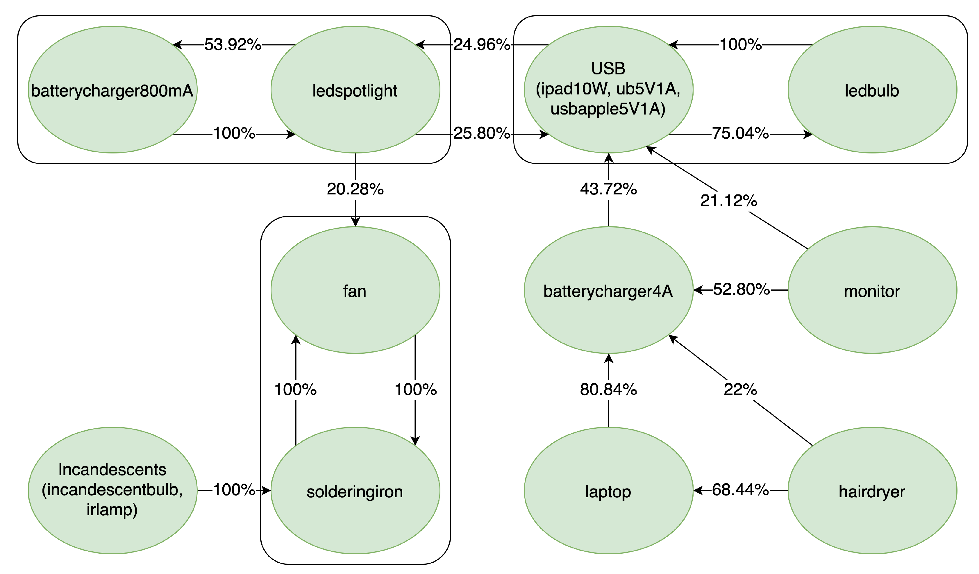
The results of the experiment are shown in Figure 3. It can be seen that there are some loads where the samples are classified into a single class, while in other cases, the samples are misclassified into a range of different classes. For example, batterycharger4A has a measurement matrix with a high standard deviation for each cell, and it has samples classified into 8 of the 10 known classes. Some classes can be thought of as a group, such as the fan and soldering iron, where both of them were classified into the other class. Based on the data, we can cluster the devices depending on where their samples had been classified to when the model had no knowledge of the class. It can be seen in Figure 4, where the clustering is shown for the TEST_ORIG profile. The USB and ledbulb form one such cluster. The reason for it may be the similar power usage level and both loads having similar power supplies.

4. Open-Set Recognition

In the previous section, we demonstrated what happens when closed classification methods encounter samples from unseen classes. Open-set recognition solves the problem of misclassification by providing means of detecting samples not belonging to any class present during the training of the model.

In [26], the difficulties and the task of open-set recognition are discussed. The goal is to find an optimal function f minimizing the loss function $L(x,y,f(x\left)\right)$:

$$arg\underset{f}{min}\left\{R_I\left(f\right):={\int }_{{\mathbb{R}}^d\times \mathbb{N}}L(x,y,f\left(x\right))P(x,y)\right\}$$

(2)

where d is the dimension of the feature vectors, y is the label of the target class, and x represents the measurements ($x\in {\mathbb{R}}^d,y\in \mathbb{N}$). The loss function has the following properties: $L(x,y,f(x\left)\right)\ge 0$ and $L(x,y,y)=0$. Minimizing the risk function $R_{\mathcal{I}}$ is a difficult task, as $P(x,y)$, the probability distribution over ${\mathbb{R}}^d\times \mathbb{N}$, is not known.

In [26], it is shown that knowledge about the known samples allows assumptions about the other parts of feature space. For example, regions located far from any known samples are less likely to contain samples from a known class.

The closed nature of classification algorithms is often disregarded in the literature. There can be various levels of openness, and thus different levels of difficulty are involved when considering open-set recognition methods. In [26], openness is defined as:

$$openness=1-\sqrt{\frac{2·\left|trainingclasses\right|}{\left|testingclasses\right|+\left|targetclasses\right|}}$$

(3)

Training classes represent the number of classes available during the training phase of the model. The number of testing classes represents the number of classes distinguished during the testing phase. The number of real-world classes to be distinguished is the target classes. Openness is 0 if samples from all classes are available during the training phase. In those cases, open-set recognition methods are not needed. However, as more unknown classes are introduced, the openness score approaches 1. In the case of load classification, the number of loads not present during training is huge compared with the number of classes that were sampled.

In [4], OpenMax is introduced as a method to enable the rejection of fooling samples in images and solve the closed nature of traditional Deep Neural Network based classification. OpenMax works by using information from values of the penultimate layer’s neurons of the DNN to adjust the SoftMax layer’s output probabilities, while also introducing another element to the output: the probability that the input is unknown. After training the Neural Network, for each known class, the means of the Activation Vectors (AVs) in the penultimate layer of the CNN are calculated. A Weibull distribution is then fitted to the norms of the differences between the AVs and the MAVs (Mean Activation Vectors). Then, during inference, the top N classes of the SoftMax layers are considered, and the probabilities are revised using the Weibull CDF probability for the selected classes. The unknown probability value is also calculated. The output of the N revised probabilities and the unknown value are normalized using the SoftMax method, and the argument of the maximum probability is selected as the decision.

4.1. Applying Open-Set Recognition to the Problem of Electrical Load Classification

No knowledge is available about the set of unknown loads when considering applying open-set detection methods to the problem of electrical load classification. When designing and choosing the parameters of the open-set-enabled classifier, only knowledge about the known classes is available, as well as the domain-specific problem statements and goals:

• Several different types of electrical loads exist, and it is infeasible to measure all of them.
• Distinguishing between individual loads achieving the same function (i.e., USB charger) is not required.
• The result of the classification is used to predict future grid load. Misclassification of a true unknown load as one of the known loads results in inaccurate predictions. Incorrectly classifying a true known load as unknown is less problematic, as no incorrect assumptions are made about the appliance’s future energy usage in those cases.
• Load control is applied to the connected electrical load via the Smart Plug. Applying load scheduling or interrupting the load’s operation because it is falsely classified as one of the known schedulable/interruptible loads can have serious consequences (i.e., turning off a device such as a hairdryer, lights, or computer).
• If a load is classified as unknown, load control is not applied, and the load can be profiled by collecting measurements. Thus, incorrectly classifying a known load as unknown does not have severe consequences compared with misclassifying an unknown load as known.

To summarize, misclassification of an unknown load should be avoided. Classifying a known load as unknown may be acceptable, provided it makes misclassification of an unseen load less likely.

5. Open-Set Recognition Using One-Class SVM

A one-class SVM classifier can be trained to predict whether a sample belongs to a class that was used during training. With this method, it is possible to detect if a known or unknown load is connected to the device. Since the one-class SVM classifier does not provide information about the specific known class, one of the classification methods shown previously ([1,3]—FCNN, SVM, CNN, and LSTM) can be used to determine the class of the sample which was detected by the one-class SVM classifier as a known sample.

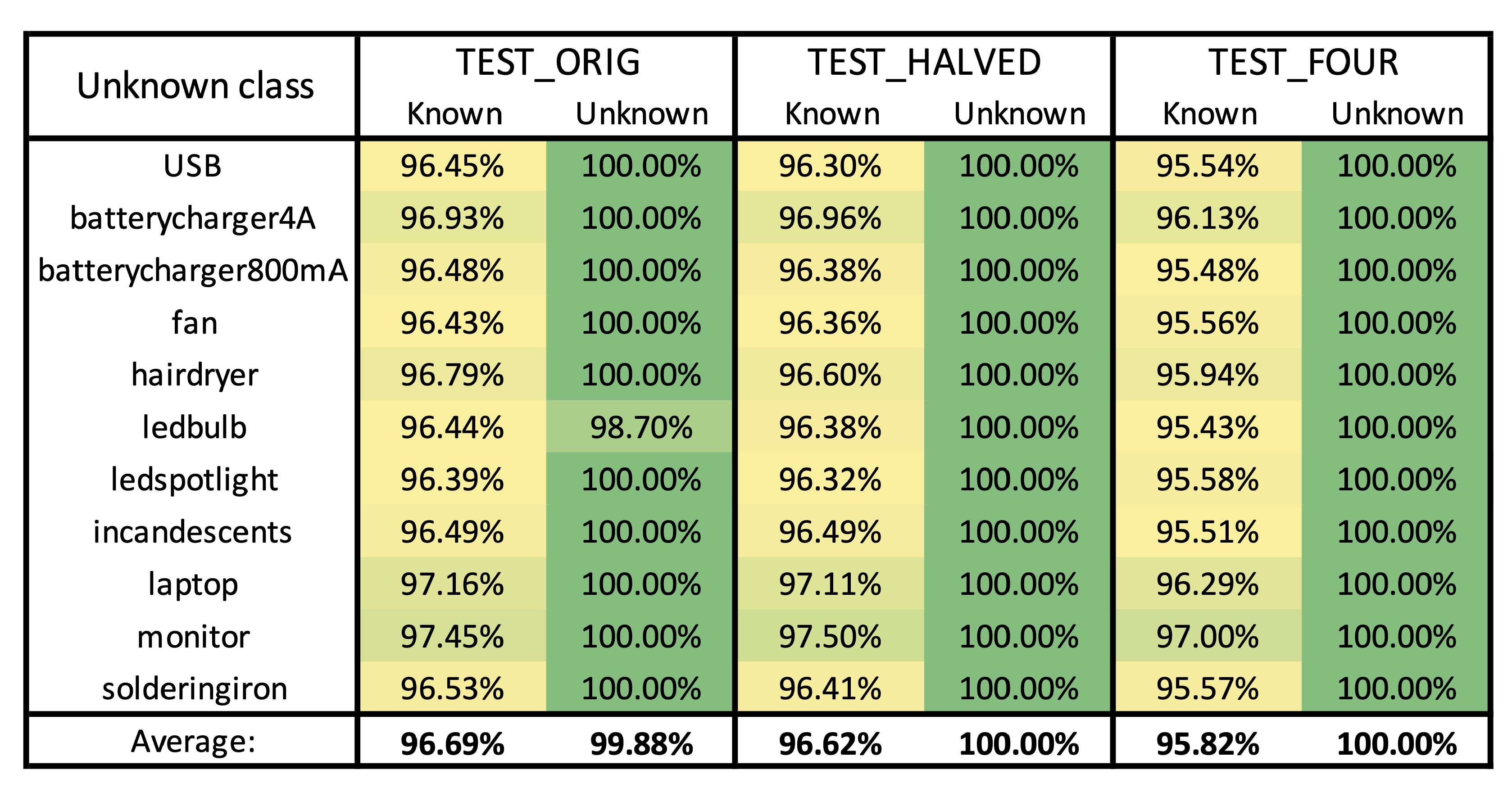
A one-class SVM classifier with an RBF (Radial Basis Function) kernel was trained, where the kernel parameter was adjusted in accordance with the requirements of the load classification problem presented in Section 4.1. The ten features introduced in Section 2.1 were used as the input of the classifier. The evaluation methodology was the following: One class was selected as the unknown class; the other classes constituted the set of known loads. Of the 250 samples per known class, 100 were used for training the model. The classifier was trained on the known training samples. Then, the model’s performance was evaluated using all 250 samples of the unknown class and the 150 unused samples from each known class. This was repeated for each class as the unknown class. The average accuracy rates (of 100 runs) are shown in Figure 5. The performance of the one-class SVM classifier was evaluated for the TEST_ORIG, TEST_HALVED and TEST_FOUR measurement profiles. The accuracy rates for the true known and unknown samples are shown in different columns. We can see that a nearly 100% rate can be achieved for the unknown samples, while for the known samples, the accuracy rates are also high, above 96% for the TEST_ORIG measurement profile.

6. Modified OpenMax Method for Open-Set Recognition

Although the one-class SVM classification presents promising results, using the ten features from Section 2.1 may not be enough in the future if the list of measured electrical loads is extended. If an unknown sample was sufficiently close to a known sample in feature space, misclassification would happen.

The modified OpenMax-based method presented in this section is more robust, using both CNN classification and the ten extracted features. The original OpenMax method [4] was examined on the dataset, but the results are much worse than the ones using the one-class SVM shown in Section 5. The problem may be that some loads, such as batterycharger4A, featured a high standard deviation in the norm from the MAV. To solve that, instead of using the MAVs and the AVs for the Weibull CDF, the ten features introduced in Section 2.1 were used for fitting the Weibull CDF for each class. This method yielded better classification results. However, in this case, normalized features such as the ratio of $2\times 2$ submatrices compared with the mean of the entire matrix contributed much less to the total norm than, for example, the mean of the input matrix values. To solve this, a mean feature vector was calculated from the known training samples, and the feature vectors were divided by this mean feature vector element-wise before the norm calculation and fitting. So, the norm was calculated the following way:

Calculating the mean feature vector for the training samples used ($TS$) for training the CNN model:

$$\mu =mean\left(T{S}_{known}\right)$$

(4)

Calculating the mean AVs for each class using the training samples from that particular class only:

$${\mu }_i=mean\left(\frac{T{S}_{knownandclass=i}}{\mu }\right)$$

(5)

Calculating the norm value for a training sample (j) belonging to class i:

$$∥\frac{T{S}_j}{\mu }-{\mu }_i∥$$

(6)

After fitting the Weibull CDF using the above normed values, during inference for a new test sample (S), the norm is calculated for each top class k using this method:

$$∥\frac{S}{\mu }-{\mu }_k∥$$

(7)

This way, there is some level of normalization, so that all ten features contribute around the same amount (on average) to the norm value for a sample.

High accuracy rates were achieved using this modified OpenMax method and setting the correct coefficients and N to be 2 (number of TOP classes to consider). The CNN consisted of two convolutional layers with 30 and 40 channels. The second layer used the SoftMax activation function to normalize the output. The convolutional layers were followed by a dropout layer (20%) and a fully connected layer with 20 neurons before the final SoftMax layer. The input consisted of the power measurement matrix of a sample.

The evaluation methodology was similar to the one-class SVM method. For each measurement profile (from TEST_ORIG, TEST_HALVED, TEST_FOUR), the following steps were executed:

1.

Select one class as the unknown class.

2.

Train the CNN model using 150 samples from each known class; no samples from the unknown class.

3.

Calculate mean feature vector, MAVs, and fit Weibull CDF for each known class.

4.

Evaluate model performance with the 100 unused known samples from each (known) class.

5.

Evaluate model performance with the 250 unknown samples from the omitted class.

6.

Repeat from step 2 for the next class as the unknown class.

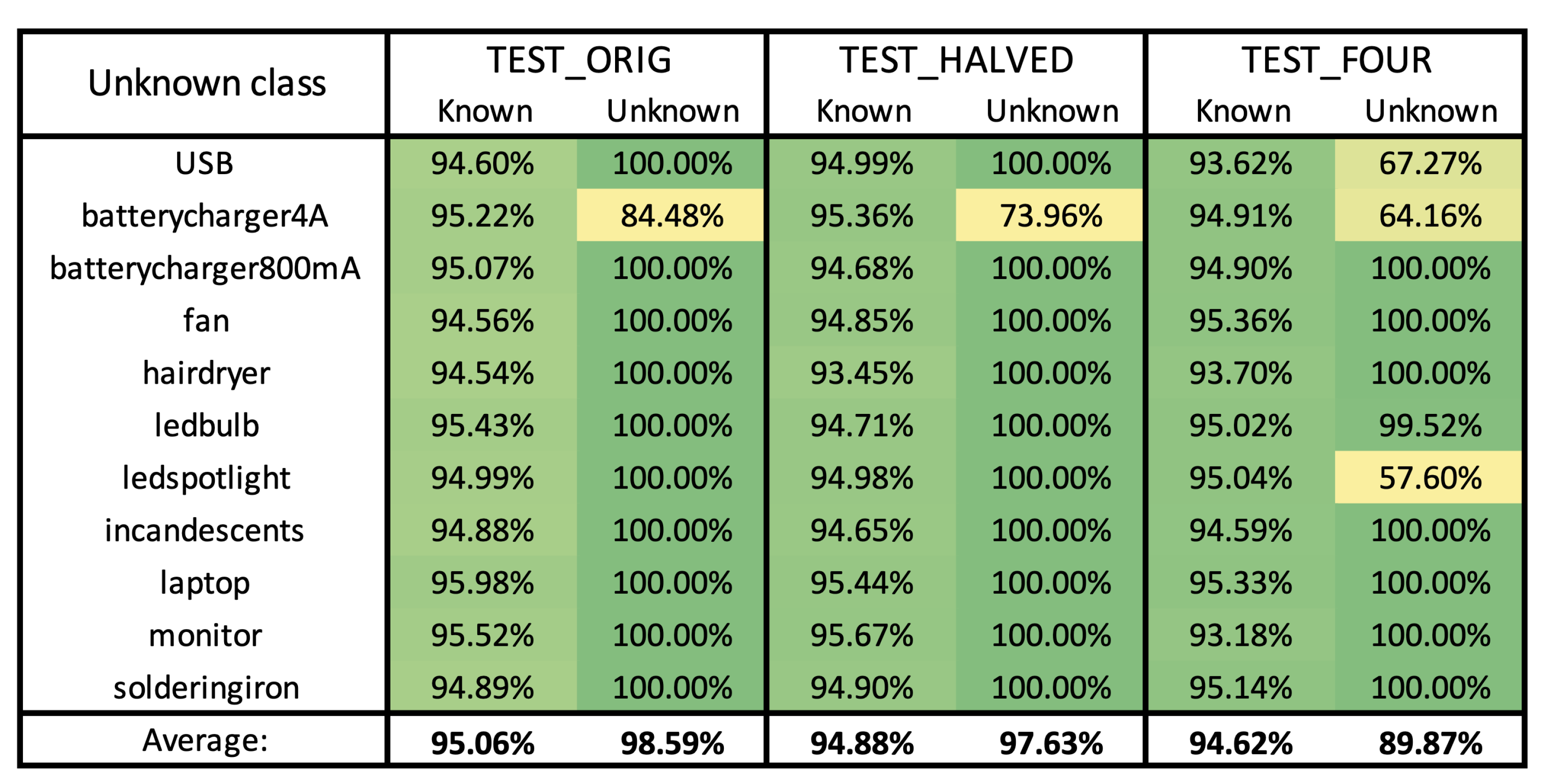
The summary of the results can be seen in Figure 6, where the averages of 10 runs are shown. We can see that the accuracy rates are slightly worse than with the one-class SVM method, but some of the errors may not be problematic with respect to load control. For the unknown samples in the case of the TEST_ORIG and TEST_HALVED measurement profiles, the only error occurred with the batterycharger4A load. For the TEST_ORIG case, 15.32% of the samples were classified as laptops, while 0.2% of the samples were classified as a monitor. In the case of load scheduling, this misclassification would not be a problem, as turning off lead–acid battery charging will not cause problems compared with other loads used, such as a hairdryer or a kitchen appliance.

7. Discussion of the Results

The results for both SVM-based and OpenMax-based open-set recognition show that the methods presented in this paper can be used to achieve accurate open-set recognition. The ability to detect previously unseen loads solves one of the often overlooked challenges of the real-world application of DSM solutions presented in the literature. The modified OpenMax-based method presented slightly lower accuracy rates, but it is a more robust method. Both solutions are suitable for detecting previously unseen electrical loads, and thus avoiding misclassification of the connected load.

For a Smart Plug such as the one introduced in [3], which is capable of on-device CNN inference, and thus electrical load classification, accommodation of further logic to enable open-set recognition would be possible. Modifying the firmware to support Weibull distribution calculation and OpenMax final layer calculation can be achieved, which will enable accurate on-device classification with open-set recognition. A Smart Plug capable of classifying a connected load in 10 s and detecting and automatically profiling unseen appliances can be a key component in a Smart Home system designed to utilize renewable resources fully.

Compared with existing proposals in the literature, our method can achieve both fast load classification and individual load control. Open-set recognition capabilities are necessary for applying load control in a real-world scenario, where training samples are not available for every electrical load in the household. Other Smart-Plug-based methods presented in the literature lack open-set recognition capabilities [9,11] or only differentiate a limited set of classes based on load characteristics [10], which would not be suitable for DSM applications. NILM methods [12,13] do not offer load control capabilities required for DSM.

With the proposed method in this paper, automatic load profiling also becomes possible. If the Smart Plug detects a previously unseen load, it can automatically profile it so that only the scheduling information will require human interaction.

The load detection and control capabilities can be used for DSM applications not only on the household level but also at the utility level. Understanding the load composition of households and the usage patterns of individual loads can be a key component in grid load estimation for energy providers. All the benefits of DSM presented in Section 2 become possible, such as better utilization of renewable energy resources and PAR reduction.

8. Conclusions and Future Work

In this paper, the applications of open-set recognition methods were discussed in the field of electrical load classification. Accurate detection of unseen loads is possible with both methods examined. This novel application of open-set recognition can enable the creation of Home Energy Management systems capable of functioning in a real-world scenario. Accurate and fast load detection is crucial for load forecasting and for effective demand-side management.

The methods presented in this paper can be applied to existing Smart Plugs in the literature (such as [3]), allowing fast on-device load classification along with open-set recognition capabilities. Smart Plugs capable of classifying a connected load within seconds and also detecting and automatically profiling unseen appliances can be a key component in a Smart Home system designed to enable full utilization of renewable resources. Renewable energy resource utilization is an especially relevant field of research due to the energy crisis in Europe. Demand-side management is a key step needed as the world transitions to using renewable energy sources. We hope our results presented in this paper become a key component to achieve that.