Computational Fluid Dynamic Simulation of Leakage Acoustic Waves Propagation Model for Gas Pipelines

Abstract

When leakage occurs for natural gas pipelines, acoustic waves generated at the leakage point will propagate to both ends of the pipe, which will be measured and processed to detect and locate the leakage. When acoustic waves propagate in the gas, the amplitude will attenuate and the waveform will spread, which decides the installation distance of acoustic sensors. Therefore, computational fluid dynamic (CFD) simulation research on the acoustic wave propagation model is accomplished and verified by experiments to provide the foundation for the acoustic leak location method. The propagation model includes two parts: amplitude attenuation model and waveform spreading model. Both can be obtained by the established CFD simulation model. Additionally, the amplitude attenuation model can be verified by the experiments. Then, the simulation method is applied to conclude the propagation model under variable conditions, including different flow directions, Reynolds numbers, and diameters. Finally, the experimental demonstration of the leak location based on the propagation model is given. The results indicate that not only the gas viscosity but also the gas flow can influence the propagation model, and the leak location method based on the propagation model is effective. Conclusions can be drawn that CFD simulation on the propagation model for natural gas pipelines is an efficient way to carry out research and provide the theoretical basis for acoustic leak location method application.

1. Introduction

At present, many leak detection and location methods [1] have been developed for gas pipelines. Among them, the acoustic method is based on the dynamic pressure monitored by the dynamic pressure sensors, which have higher sensitivity, higher location accuracy, lower false alarm rate, shorter testing time, and greater adaptability. The fundamental of the acoustic method is that when leakage occurs, the acoustic waves generate which propagate to upstream and downstream and are captured by the acoustic sensors. Then, the leakage signals are processed by computer to detect and locate the leakages.

Though the acoustic method has many advantages, its popularization and application are restricted by the installation distance or cost of acoustic sensors, which is decided by the propagation characteristics. A group of scholars conducted research on leak detection and location based on acoustic waves. Osama [2] collected leakage acoustic signals propagating in the medium inside plastic water pipes and propagating through the pipe wall using microphones and accelerometers, respectively. The experimental results show that the amplitude of signals attenuates with the propagation distance at the speed of 0.25 dB/m, and the propagation velocity of signals whose frequency is lower than 50 Hz is independent of frequency, and acoustic signals propagate faster by 7% in winter than in summer. Muggleton [3] analyzed the mechanism of the propagation behavior of sound and vibration waves caused by leakage of a fluid-filled round pipeline and established the propagation model of signals and analyzed the attenuation characteristics of the acoustic signals. Prek [4] describes the investigation of the propagation wave speed and wave attenuation in viscoelastic fluid-filled pipes. The frequency-dependent wave speed and attenuation were calculated from the transfer function between three pressure measurements. The experimental results for different pipe wall materials, particularly those with applications in water supply installations, are presented. Mostafapour [5] studied the leak acoustics generated by pipe wall vibration through simulation, which propagated as the form of pressure wave and can be measured by the sensors installed into the pipe wall. Then, the propagation law was researched through theoretical and experimental analyses, which provide the foundation for leak detection and location for natural gas pipelines. Mostafapour [6] carried out a theoretical and experimental study on acoustic signals caused by leakage in buried gas-filled pipe. The standard form of the Donnell’s non-linear shallow shell equation is used to model the free vibration of the pipe, and the effects of the surrounding medium on the pipe radial displacement is modeled by the potential function.

Liu [7] studied the propagation model of acoustic waves. Then, the fundamental characteristics of leakage acoustic waves are obtained by time-domain, frequency-domain, and joint time-frequency-domain analyses. Almeida [8] accomplished a study towards an in situ measurement of wave velocity in buried plastic water distribution pipes for the purposes of leak location. Brennan [9] designed a virtual pipe rig for testing acoustic leak detection correlators by which leak noise propagating in buried water pipes has been determined. Yu [10] presented an experimental investigation on acoustic emission (AE) based small leak detection of galvanized steel pipe due to screw thread loosening. The waveform, frequency, and energy signatures of the AE signals were extracted and compared. Gao [11] studied an axisymmetric fluid-dominated wave in fluid-filled plastic pipes considering the effects of the surrounding elastic medium. The analysis was extended to investigate the loading effects of the surrounding medium on the low-frequency propagation characteristics. Butterfield [12] accomplished an experimental investigation into vibro-acoustic emission-signal-processing techniques to quantify leak flow rate in plastic water distribution pipes. Gao [13] improved the shape of the cross-correlation function for leak detection in a plastic water distribution pipe using acoustic signals. She dealt with time delay estimation for the detection of leaks in buried plastic water pipes using the cross-correlation of leak noise signals. Brennan [14] researched on the effects of soil properties on leak noise propagation in plastic water distribution pipes. He carried out an analytical, numerical, and experimental investigation into the way soil properties influence leak noise propagation in buried plastic water pipes.

From the research on the acoustic leak detection method, it can be concluded that the propagation model, including the amplitude attenuation and waveform spreading, has not been studied. In addition, there are many limitations of the present research. In this view, the acoustic leak location method, including the propagation model, is studied by the combination of simulation [15] and experimental methods. The simulation and experimental models are proposed and designed. The three-dimensional (3-D) time-domain pulse method is established through which the propagation model, including attenuation coefficients and time coefficients of acoustic waves, can be obtained. Propagation characteristics under different conditions are simulated. Then, the propagation model is applied for leak location by which the method based on the amplitude attenuation model is proposed.

2. Theoretical Analysis

Nowadays, the main methods to study the propagation characteristics of acoustic waves in fluid pipelines are the frequency-domain method and the time-domain method. The former one includes the plane wave transfer matrix method, two- and three-dimensional analytical method, finite element method, and boundary element method. These methods find solutions to the linear wave equation in frequency domain. They have relatively simple formulas and fast calculation speeds, while it is difficult for them to take the influences of the medium viscosity and the complex flow into consideration. To solve the problems, the time domain method is proposed, which can calculate the pressure fluctuations of the inlet and outlet boundary of the pipeline in time-domain by the computational fluid dynamics (CFD) method and then obtain the propagation loss.

2.1. CFD Method in Time-Domain

The propagation process of the acoustic waves in the fluid pipeline is a kind of fluid dynamics. Therefore, it is feasible to study the acoustic performances by the CFD simulation technique based on the basic equations of fluid dynamics. It has obvious advantages over the frequency domain method, which takes the effects of nonlinear factors into consideration, such as heat conduction, viscosity, complex flow field. As known to all, the CFD calculation includes the establishment of governing equations, the determination of boundary and initial conditions, the discrete calculation domain and control equations, the determination of solution methods and iterative solutions. The control equations are dependent on the continuity equation, momentum equation, and energy equation [16]. The turbulent model is chosen as the standard $k-\epsilon$ model. Moreover, the boundary conditions are set as the inlet and outlet pressure boundaries. The pipe wall is set as the wall with no slip under the adiabatic condition, which makes the sound wave propagate in the gas as the form of plane wave.

2.2. The Calculation Method of Propagation Loss

There are two methods to calculate the propagation loss by CFD method: pressure pulse method and acoustic wave decomposition method. The former one simulates the propagation process of the pressure pulse. The pressure changes with time at the inlet and outlet boundaries of the pipe are recorded, respectively. The later one applies the white noise signal as the inlet condition to simulate the signal transmission process.

The propagation loss can be described through two indexes. One is the ratio of the acoustic power in frequency domain; the other is the ratio of the acoustic amplitude in time domain.

In this paper, the pressure pulse method with the ratio of the acoustic amplitude in time domain is applied.

2.3. Establishment of Three-Dimensional (3-D) Time-Domain Pulse Method

The acoustic characteristics can be portrayed by the 3-D CFD model in which it is necessary to enter the acoustic source as the inlet boundary. Additionally, the outlet boundary should keep constant with the actual acoustic characteristics. The mesh size and time step should be set to capture the tiny fluctuations in acoustic magnitude. In this view, the 3-D time-domain pulse method is proposed, which is used to calculate the propagation characteristics.

For the proposed method, it is important to figure out the acoustic source as the inlet boundary.

When leakage occurs for natural gas pipelines, the acoustic waves generate, and the waveforms can be fitted, as shown in Equation (1).

$$\Delta p=\left\{\begin{array}{l}0,\hspace{1em}\hspace{1em}\hspace{1em}\hspace{1em}t\le t_x\\ -p_0{\mathrm{e}}^{-\left(t-t_x\right)/t_0},\hspace{1em}t>t_x\end{array}\right.$$

(1)

where $\Delta p$ is the acoustic amplitude, kPa; $p_0$ is the initial acoustic amplitude, kPa; $t_x$ is the leakage occurring time, s; $t_0$ is the time constant, s.

Then, Equation (2) can be obtained from Equation (1), and it can be used as the pressure inlet boundary condition, which will be achieved through the user-defined functions (UDF) in CFD software.

$$p=\left\{\begin{array}{l}{p}_{in},\hspace{1em}\hspace{1em}\hspace{1em}\hspace{1em}\hspace{1em}t\le t_x\\ p_{in}-p_0{\mathrm{e}}^{-\left(t-t_x\right)/t_0},\hspace{1em}t>t_x\end{array}\right.$$

(2)

where $p$ is the inlet pressure, Pa; $p_{in}$ is the average pressure level, Pa; $p_0$ is the acoustic amplitude, Pa; $1/t_0$ can be called as the time coefficient (TC) which describes the rising section of waves. The latter two can be obtained in Table 1 by fitting experimental signals.

Table 1. Acoustic amplitudes and TCs.

Pressure /kPa	Leakage Orifice/mm	Fitted Signals			Simulated Values
		Acoustic Amplitude/Pa	Leakage Time/s	TCs/10−4 s	Acoustic Amplitude/Pa	Leakage Time/s	TCs/s
1150	0.6	−13,089.05	16.767	3.871	−2,042,173.8	0.01	−500
	0.7	−15,306.29	11.402	3.649	−2,388,074.2	0.01	−500
	0.8	−14,094.59	15.105	4.090	−2,199,132.6	0.01	−500

Equation (2) shows the acoustic source form of the inlet boundary when the acoustic waves propagate downstream. Likewise, when the acoustic waves propagate upstream, the acoustic source form of the outlet boundary can be described as Equation (3).

$$p\prime =\left\{\begin{array}{l}{p}_{out},\hspace{1em}\hspace{1em}\hspace{1em}\hspace{1em}t\le t_x\\ p_{out}-p_0{\mathrm{e}}^{-\left(t-t_x\right)/t_0},\hspace{1em}t>t_x\end{array}\right.$$

(3)

where $p\prime$ is the outlet pressure, Pa; $p_{out}$ is the average pressure level, Pa; $p_0$ and $1/t_0$ can be obtained in Table 1 by fitted signals.

The calculation steps of the proposed method are shown as follows.

(1) Steady state calculation is carried out to obtain the flow field distribution; at this time, the fixed pressure level can be regarded as the inlet boundary, and the other pressure value can be regarded as the outlet boundary. The pressure difference should result in the gas velocity which equals the experimental one. (2) Based on step (1), the transient calculation without pulse is carried out. The monitoring points are set to capture the pressure changes. (3) Based on step (1), the transient calculation with pulse is carried out. The pressure inlet boundary condition can be set as Equation (2) when acoustic waves propagate downstream, or the pressure outlet boundary condition can be set as Equation (3) when acoustic waves propagate upstream. In addition, the same monitoring points are set to capture the pressure changes. (4) The pressures obtained in step (3) minus the ones obtained in step (2) at the same point are the pressure pulse after removal of static pressure, which are also regarded as acoustic waves.

In calculation of the acoustic wave propagation process, the reflection at the outlet of the pipe should be taken into consideration. To eliminate it, one method is that the outlet boundary condition can be set as the pressure far field. However, after the test, it can be found that the method wastes long computing time. The other way is to use the pressure outlet boundary with an appropriate pipeline length and the simulation time during which the acoustic wave can not reach the outlet from the inlet. Therefore, the reflection can not generate. Because the acoustic velocity is fast, if the TC is used as shown in Table 1, the pipeline length will become large, which will contribute to a large calculation amount. To solve the problem, Equation (2) should be scaled to Equation (4), and simulated values are used.

$$p=\left\{\begin{array}{l}{p}_{in},\hspace{1em}\hspace{1em}\hspace{1em}\hspace{1em}t\le t_x\\ p_{in}-p_0^{\prime }{\mathrm{e}}^{-t/t_0},\hspace{1em}t>t_x\end{array}\right.$$

(4)

As a result, the new acoustic amplitudes and TCs of simulated values are shown in Table 1 when the pipe of the simulation model is 30 m.

3. Simulation Analysis

The FLUENT CFD software will be utilized for the simulation. The applied process is model, mesh, setup, solution, and results.

3.1. Establishment of Simulation Model

The simulation model is established as shown in Figure 1.

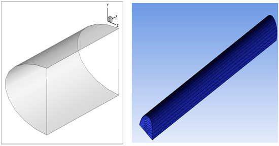
Figure 1. The propagation model of acoustic waves in the gas pipeline.

Figure 1 shows that the physical model is a pipe section of which the length is 30 m, and the diameter is 10 mm. The gas flowing through the pipeline is compressible ideal air, which inlets from the left-side end of the main pipe and outlets from the right-side end. The monitoring points located at the centerline are 10 m, 12.5 m, 15 m, 17.5 m, and 20 m far from the left-side end. When the operating pressure of the pipeline is 1150 kPa with a 0.8 mm leakage orifice, the boundary conditions are set as follows: the inlet condition is the pressure inlet, and the pressure is described as Equation (5); the outlet is the pressure outlet, and the pressure is 1,149,800 Pa. In addition, the realizable two equation turbulence model is applied.

$$p=\left\{\begin{array}{l}\mathrm{1,150,000},\hspace{1em}\hspace{1em}\hspace{1em}\hspace{1em}\hspace{1em}t\le 0.01\\ \mathrm{1,150,000}-\mathrm{2,199,132.6}{\mathrm{e}}^{-500t},\hspace{1em}t>0.01\end{array}\right.$$

(5)

Because the model is symmetric, to reduce the computation amount, the symmetric model is applied. When the mesh size is set as 1, 2, and 4 mm, the number of the grids is 795,000, 375,000, 162,000, with the calculation consequence of 1,150,000, 114,990, 114,000. Considering the calculation precision and time, the mesh size is set as 2 mm by which it can be ensured that there are at least six grid units in one wavelength to improve the accuracy of the calculation. In addition, the time independence verification is carried out, which is set as 25 μs.

3.2. Flow Field Analysis Obtained by CFD Simulation

The viscosity and flow of gas are the main reasons which contribute to the amplitude attenuation and waveform spreading. Therefore, in simulation, viscosity is firstly taken into consideration and then flow. The simulation models at 1150 kPa with 0.8 mm leakage orifice are shown as Table 2.

Table 2. Simulation models.

Simulation Model	Steady State Calculation Model	Transient State Calculation Model	Inlet Pressure/Pa	Outlet Pressure/Pa
Non-viscosity and static flow	No	Inviscid	Equation (5)	1,150,000
Viscosity and static flow	No	Laminar flow	Equation (5)	1,150,000
Non-viscosity and flow	Yes	Inviscid	Equation (5)	1,149,800
Viscosity and flow	Yes	Realizable $k-\epsilon$	Equation (5)	1,149,800

Then, all simulation models are applied to study the propagation characteristics. In addition, the simulation model of viscosity and flow is taken for an example to be described in detail.

3.2.1. Acoustic Waves Propagate Downstream

The steady-state calculation is performed firstly as the inlet pressure is 1,150,000 Pa, and the outlet pressure is 1,149,800 Pa; velocity is 5.36 m/s. After 2000 iterations, the transient calculation is carried out: the time step size is $2.5\times {10}^{-5}$ s; number of time steps is 3530; the total simulation time is 0.08825 s. After 2000 iterations, the transient calculation with pressure pulse is carried out: the inlet pressure is set as Equation (5) by UDF which can be seen in Figure 2.

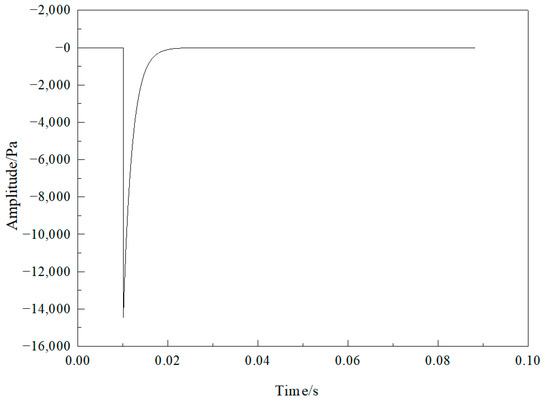
Figure 2. The inlet-pressure boundary condition.

When there is no pressure pulse as inlet, the pressure distribution can be seen in Figure 3.

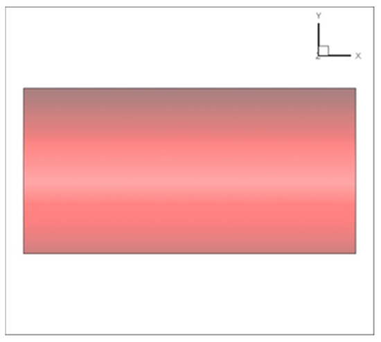
Figure 3. Pressure distribution without pressure pulse as inlet.

After the simulation with pressure pulse is accomplished, the propagation process can be obtained as shown in Figure 4.

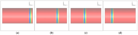
Figure 4. Pressure distribution when the pulse propagates in the pipe (blue represents the amplitude): (a) 0.02 s, (b) 0.04 s, (c) 0.06 s, (d) 0.08 s.

The pressure is stable before 0.01 s, and there is a negative pressure zone in the pipe with the input of pressure pulse. The negative pressure zone shows regular pressure layers between which the interfaces are plane. The moving speed of the zone is acoustic velocity. Because the boundary layer of the pipe wall is not considered, the acoustic wave propagates in the form of a standard plane wave. Additionally, in the propagation process, the negative pressure zone becomes wider, especially the front of the zone.

Pressure at the monitoring points without pulse inlet is subtracted from pressure at the corresponding monitoring points with pulse inlet. The results are acoustic pressure amplitude variation, as shown in Figure 5.

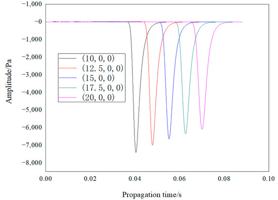
Figure 5. Amplitude changes of acoustic pressure.

Acoustic amplitude attenuates with the increase of the propagation distance, and the amplitudes are shown in Table 3.

Table 3. Amplitudes and TCs at different monitoring points.

Propagation Distance/m	Drop Points	Amplitude /Pa	Amplitude Corresponding Point	Difference Value	1/TC /(1/s)	TC/s	Coefficient of Curve Fitting
10	1450	−7414.63	1618	168	497.82	0.002009	0.9994
12.5	1732	−6998.25	1915	183	497.57	0.002010	0.9991
15	2011	−6653.75	2211	200	497.20	0.002011	0.9987
17.5	2299	−6360.50	2507	208	496.51	0.002014	0.9983
20	2583	−6106.13	2803	220	494.05	0.002024	0.9979

After being fitted, with the increase of the propagation distance, the amplitude attenuation follows the exponential law of which the attenuation coefficient (AC) is 0.019355.

From Table 3, it can be seen that the difference between the amplitude corresponding point and the drop point becomes larger with the increase of distance, which shows that the drop sections in Figure 5 become smoother. This is consistent with the fact that the front of the negative pressure zone grows wider. However, the growth rate has no obvious rule.

The TC increases with the increase of propagation distance, and increasing law complies with Equation (6):

$$t_0=0.0020e^{0.00046x}$$

(6)

3.2.2. Acoustic Waves Propagate Upstream

The steady-state calculation is performed firstly. The inlet-pressure is 1,150,000 Pa, and outlet-pressure is 1,149,800 Pa; velocity is 5.36 m/s. After 2000 iterations, transient calculation is carried out. the time step size is $2.5\times {10}^{-5}$ s; number of time steps is 3530; the total simulation time is 0.08825 s. After 2000 iterations, the transient calculation with pressure pulse is carried out. The outlet-pressure is set as Equation (7) by UDF which can be seen in Figure 6.

$$p=\left\{\begin{array}{l}\mathrm{1,149,800},\hspace{1em}\hspace{1em}\hspace{1em}\hspace{1em}\hspace{1em}t\le 0.01\\ \mathrm{1,149,800}-\mathrm{2,199,132.6}{\mathrm{e}}^{-500t},\hspace{1em}t>0.01\end{array}\right.$$

(7)

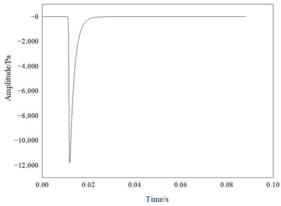
Figure 6. The outlet-pressure boundary condition.

After the simulation with pressure pulse is accomplished, the propagation process can be obtained as shown in Figure 7.

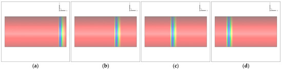
Figure 7. Pressure distribution when the pulse propagates in the pipe when acoustic waves propagate upstream (blue represents the amplitude): (a) 0.02 s, (b) 0.04 s, (c) 0.06 s, (d) 0.08 s.

The pressure is stable before 0.01 s, and there is a negative pressure zone in the pipe with the input of pressure pulse. The negative pressure zone shows the same laws with the one of the acoustic waves propagating downstream.

The acoustic pressure amplitude variations are shown in Figure 8.

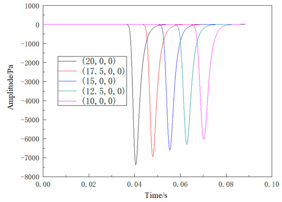
Figure 8. Amplitude changes of acoustic pressure when acoustic waves propagate upstream.

The amplitude changes are shown in Table 4.

Table 4. Amplitudes and TCs at different monitoring points when acoustic waves propagate upstream.

Propagation Distance/m	Drop Points	Amplitude/Pa	Amplitude Corresponding Point	Difference Value	1/TC/(1/s)	TC/s	Coefficient of Curve Fitting
10	1454	−7369.38	1621	167	517.51	0.001932	0.9987
12.5	1733	−6945.38	1918	185	517.71	0.001932	0.9981
15	2018	−6594.88	2215	197	518.50	0.001929	0.9974
17.5	2298	−6294.50	2512	214	520.12	0.001923	0.9965
20	2585	−6031.88	2809	224	522.86	0.001913	0.9954

After being fitted, with the increase of the propagation distance, the amplitude attenuation follows the exponential law of which the AC is 0.019958.

The same conclusions with the ones from Table 3 can be drawn from Table 4.

The TC increases with the increase of propagation distance, and the increasing law complies with Equation (8):

$$t_0=0.0020e^{-0.00245x}$$

(8)

3.3. Validation of the Simulation Results with the Experimental Data

The experimental loop is established, and the acoustic data are measured through dynamic pressure sensors.

3.3.1. Establishing the Experimental Facility

A high-pressure gas pipeline loop with leak detection system is designed and established by similarity analysis with field transportation pipelines, as seen in Figure 9. With an internal diameter of 10 mm, the length of the test pipeline is 200.70 m. Five leakage points are located where the valve and orifice plate are installed to control the leak flow rate from the orifice. The diameter of the orifice is variable with 0.10 mm, 0.45 mm, 0.90 mm. Dynamic pressure sensors are applied to measure signals, which should be installed with the diaphragm horizontal.

Figure 9. High-pressure gas pipeline leak detection and location device based on acoustic method.

The experiments include two parts according to the gas flow direction. (1) The acoustic waves propagate downstream which are measured by sensors 1, 2, 3, 4 when leakage point 1 leaks. The distances between sensors and leakage point 1 are respectively 0.1 m, 48.3 m, 109.1 m, 160.49 m. (2) The acoustic waves propagate upstream which are measured by sensors 4, 3, 2, 1 when leakage point 5 leaks. The distances between sensors and leakage point 5 are respectively −0.1 m, 60.7 m, 108.9 m, 151.11 m. In each part, the experiments are carried out at 1 MPa, 2 MPa, 3 MPa, 4 MPa, 5 MPa.

3.3.2. Analyzing of Experimental Data

At 1 MPa with 0.45 mm, the four signals measured by sensors can be seen in Figure 10.

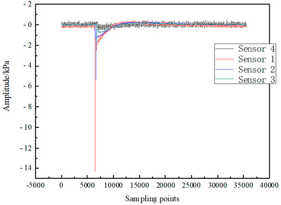
Figure 10. The acoustic signals measured by the sensors in the same direction.

From Figure 10, the waveforms remain similar and spread, and the amplitude attenuates as the acoustic waves are in the propagation process.

Then, ACs under 1 MPa can be obtained in Table 5.

Table 5. The fitted ACs when acoustic waves propagate downstream.

Pressure/MPa	Leakage Orifice/mm	Distance/m	Amplitude/kPa	ACs	Average
1	0.1	0.1	−12.48503	0.020119	0.020861
		48.3	−4.63913
		109.1	−1.54617
		160.49	−0.47318
	0.45	0.1	−14.27095	0.020796
		48.3	−5.35099
		109.1	−1.77649
		160.49	−0.47906
	0.9	0.1	−22.47467	0.021669
		48.3	−8.76786
		109.1	−2.89263
		160.49	−0.64574

From Table 5, though the leakage orifices change, the ACs change little and the average one can represent AC under 1 MPa. This fact means the ACs can be regarded as constant with the leakage orifices. Likewise, when the acoustic waves propagate upstream, ACs under 1 MPa can be obtained in Table 6.

Table 6. The fitted ACs when acoustic waves propagate upstream.

Pressure/MPa	Leakage Orifice/mm	Distance/m	Amplitude/kPa	ACs	Average
1	0.1	−0.1	−21.63334	0.023398	0.023027
		60.7	−4.25644
		108.9	−1.53141
		151.11	−0.61887
	0.45	−0.1	−17.74594	0.022693
		60.7	−3.72122
		108.9	−1.54179
		151.11	−0.53928
	0.9	−0.1	−19.03354	0.022990
		60.7	−3.87986
		108.9	−1.54738
		151.11	−0.55907

The same conclusions can be drawn from Table 6 as Table 5.

As the analyses above, the ACs obtained by simulation and experiments under five pressure levels can be seen in Table 7.

Table 7. The ACs when acoustic waves propagate downstream and upstream.

Pressure/ kPa	Downstream				Upstream
	Gas Velocity /m/s	ACs by Simulation	ACs by Experiment	Errors/%	Gas Velocity/m/s	ACs by Simulation	ACs by Experiment	Errors/%
1150	5.465	0.019355	0.020861	−7.22	5.448	0.021958	0.023027	−4.64
2050	3.386	0.013107	0.014479	−9.48	3.315	0.015702	0.016260	−3.43
3170	2.291	0.009680	0.009791	−1.13	2.238	0.011478	0.012376	−7.26
4060	1.295	0.006680	0.007016	−4.79	1.274	0.008656	0.009122	−5.11
5060	1.488	0.006532	0.006963	−6.19	1.423	0.008586	0.009500	−9.62

From Table 7, conclusions can be drawn as follows:

(1)

When acoustic waves propagate downstream, compared with ACs obtained by experiments, the errors of the ones obtained by simulation are smaller than 10%. Additionally, the ACs obtained by experiments are larger than the ones obtained by simulation.

(2)

When acoustic waves propagate upstream, compared with ACs obtained by experiments, the errors of the ones obtained by simulation are smaller than 10%. In addition, the ACs obtained by experiments are larger than the ones obtained by simulation.

The reasons are mainly as follows. In simulation, the ACs are affected by gas flowing and gas absorption, while in experiment besides the two points, the ACs are also affected by the friction between the acoustic waves and pipe wall. Additionally, the bend pipes and valves both contribute to more resistance for acoustic waves propagation.

Though errors exist, they are small enough. It can be concluded that ACs obtained by simulation can be verified by experiments. The experimental results of waveform spreading show that when acoustic waves propagate, they spread though there are noises which leads to the waveform-spreading speed only being calculated by simulation. In a word, the simulation method in this paper can be applied to study the propagation model of acoustic waves.

Then, propagation characteristics under different conditions in Table 2 can be obtained. The simulation models are at 1150 kPa with 0.8 mm leakage orifice, which are the same as the conditions of the experiment at 1150 kPa in Table 7. Whether the gas flowing or viscosity is considered or not, the acoustic waves propagate downstream or upstream, and the differences between amplitude corresponding points and drop points get larger with the increase of distance, which shows that the drop sections of acoustic waves become smoother.

The amplitude attenuation and TC changing both comply with the exponential law of which the results can be seen in Table 8.

Table 8. Propagation characteristics obtained by different simulation models.

Simulation Model	Direction	Distance/m	ACs	TCs/s	TCs Factors
Non-viscosity and static flow	--	0	0.017872	0.002000	0.00089
		10		0.002012
		12.5		0.002018
		15		0.002024
		17.5		0.002032
		20		0.002043
Viscosity and static flow	--	0	0.019015	0.002000	0.00222
		10		0.002059
		12.5		0.002065
		15		0.002070
		17.5		0.002075
		20		0.002081
Non-viscosity and flow	Downstream	0	0.017518	0.002000	0.00060
		10		0.002004
		12.5		0.002011
		15		0.002017
		17.5		0.002022
		20		0.002030
	Upstream	0	0.017647	0.002000	0.00097
		10		0.002013
		12.5		0.002021
		15		0.002028
		17.5		0.002035
		20		0.002045
Viscosity and flow	Downstream	0	0.019355	0.002000	0.00046
		10		0.002009
		12.5		0.002010
		15		0.002011
		17.5		0.002014
		20		0.002024
	Upstream	0	0.019958	0.002000	−0.00245
		10		0.001932
		12.5		0.001932
		15		0.001929
		17.5		0.001923
		20		0.001913

From Table 8, several conclusions can be drawn as follows:

(1)

For amplitude ACs, compared with the non-viscosity and static flow model, the ones of the viscosity and static flow model become larger due to viscosity, while the ones of non-viscosity and flow models become smaller due to gas flow, which shows that the influence of viscosity is much larger than the one of gas flow. Compared with the viscosity and static flow model, the ones of the viscosity and flow models become larger due to gas flow. The former two comparative analyses show that the existence of viscosity makes the opposite influences of gas flow, and the ones obtained when downstream are smaller than the ones obtained when upstream.

(2)

For TCs and their factors, with the increase of distance, TCs of the non-viscosity and static flow model become larger of which the law obeys exponential function. The viscosity makes the TCs factor much larger. When gas flow was introduced without viscosity, downstream helped to keep the waveform, while upstream aggravates the waveform change, and the influence of downstream is larger than the one of upstream. Then, viscosity is taken into consideration. It can be found that when downstream, viscosity help to keep the waveform, while when upstream viscosity aggravates the waveform change. In a word, compared with the results of the non-viscosity and static flow model, viscosity makes the smoothing speed of the rising section become larger; gas flow has different changing speeds of the rising section according to different directions. Generally, the rising section becomes smooth though downstream reduces the smoothing trend, while upstream enhances the trend. The Reynolds number can combine the influences of viscosity and gas flow.

3.4. Simulation Analysis under Variable Conditions

3.4.1. Simulation under Different Reynolds Numbers

To describe the effects of Reynolds numbers, methane and nitrogen are selected of which the parameters are in Table 9.

Table 9. Parameters of different gases.

Gas	Kinematics Viscosity under Normal Condition/10−5	Velocity/(m/s)	Reynolds Numbers
Air	1.711	5.362	3024.224
Nitrogen	1.663	5.452	3161.373
Methane	1.027	7.207	6738.122

The results can be seen in Table 10.

Table 10. The ACs and TCs under different Reynolds numbers.

Reynolds Numbers	Direction	AC	TCs Factors
3024	Downstream	0.019355	0.00046
	Upstream	0.019958	−0.00245
3161	Downstream	0.019204	0.00110
	Upstream	0.019871	−0.00233
6738	Downstream	0.018082	0.00242
	Upstream	0.018984	−0.00194

In Table 10, ACs get smaller as the Reynolds numbers get larger, which verifies the conclusion that the larger the viscosity is, the larger the AC is.

At the same time, the TCs factors are obtained. When downstream, the TCs factors are positive, which means the rising section of waveforms becomes smooth. They become larger as the Reynolds numbers becomes larger, which means the smooth speed of the rising section of waveforms become larger. These facts tell that as the Reynolds numbers become larger, it is more difficult to keep the waveform. The conclusion is verified by the one the viscosity helps to keep the waveform drawn from simulation of viscosity and flow downstream model. When upstream, the TCs factors are negative, and their absolute values become smaller as the Reynolds numbers become larger, which means as the Reynolds numbers become larger, it is more helpful to keep the waveform.

3.4.2. Simulation under Different Diameters

Then, the other two diameters are used to calculate the ACs by simulation of which the results can be seen in Table 11.

Table 11. ACs under different diameters.

Diameter/mm	Direction	ACs
20	Downstream	0.014787
	Upstream	0.014971
10	Downstream	0.015905
	Upstream	0.016532
8	Downstream	0.017072
	Upstream	0.017898

In Table 11, ACs become larger as the diameter get smaller.

4. Application of Propagation Model

After the propagation model is established, ACs are calculated, which can be used for leak location. When leakage occurs, the acoustic waves generate and propagate upstream and downstream. If sensors are installed, the amplitude of acoustic waves can be obtained as:

$$p_1=p_0\exp \left(-{\alpha }^{-}\left|x\right|\right)$$

(9)

$$p_2=p_0\exp \left[-{\alpha }^{+}\left(L-\left|x\right|\right)\right]$$

(10)

Then, leak location can be achieved by the following equation:

$$\left|x\right|=\frac{\ln \left(p_2/p_1\right)+{\alpha }^{+}L}{{\alpha }^{+}+{\alpha }^{-}}$$

(11)

where $p_1$ is the amplitude of signal measured by the upstream sensor, and $p_2$ is the one measured by downstream sensor, kPa; $L$ is the distance between two sensors, m; ${\alpha }^{+}$ is the attenuation coefficient when wave propagates downstream, while ${\alpha }^{-}$ is the one when wave propagates upstream, both of which can be obtained by simulation and experiments, as shown in Table 7.

Then, facilities in Figure 9 are used to carry out experiments. In this situation, leakage point 2 leaks. Sensor 1 is located upstream, the distance between it and leakage point 2 is 48.0 m. Sensors 2, 3, 4 are located downstream, the distances between them and sensor 1 are 48.2 m, 109 m, and 160.39 m, respectively. The results can be seen in Table 12.

Table 12. Leak location results based on propagation model.

Pressure/ kPa	Leakage Orifice/mm	Number of Sensors	Distance between the Sensor and Sensor 1/m	Sampling Point	Amplitude /kPa	Location by ACs by Simulation		Location by ACs by Experiments		Location by Traditional Method
						Location Point	Location Error	Location Point	Location Error	Location Point	Location Error
				11,765	−5.341
		3	48.20	11,621	−15.771	48.790	1.639	47.582	−0.867	47.998	−0.005
		4	109.00	11,797	−4.959	49.270	1.165	50.120	1.945	47.646	−0.325
		5	160.39	11,948	−1.571	45.522	−1.545	48.359	0.224	47.452	−0.342
	0.45	2		9755	−5.137
		3	48.20	9615	−15.098	48.677	1.405	47.474	−1.091	47.827	−0.360
		4	109.00	9789	−4.648	48.645	0.592	49.529	1.403	47.988	−0.011
		5	160.39	9938	−1.592	46.786	−0.757	49.549	0.966	47.452	−0.342
	0.9	2		14,438	−5.342
		3	48.20	14,297	−15.494	48.357	0.740	47.173	−1.716	47.998	−0.005
		4	109.00	14,470	−4.864	48.797	0.731	49.676	1.538	47.475	−0.482
		5	160.39	14,621	−1.554	45.254	−1.712	48.096	0.060	10.516	−23.371
2	0.1	2		16,813	−11.038
		3	48.20	16,674	−23.248	47.785	−0.446	46.936	−2.207	47.909	−0.189
		4	109.00	16,848	−10.570	48.087	0.080	49.933	1.773	47.957	−0.039
		5	160.39	16,999	−4.309	40.321	−4.788	44.946	−1.904	47.297	−0.438
	0.45	2		16,035	−13.396
		3	48.20	15,896	−29.846	49.736	3.602	48.763	1.584	47.909	−0.189
		4	109.00	16,070	−12.106	46.076	−1.765	48.048	0.044	48.129	0.119
		5	160.39	16,220	−5.203	40.144	−4.898	44.779	−2.009	47.469	−0.331
	0.9	2		11,896	−12.217
		3	48.20	11,754	−25.864	47.964	−0.076	47.104	−1.859	47.909	−0.189
		4	109.00	11,930	−11.456	47.358	−0.589	49.251	1.148	47.957	−0.039
		5	160.39	12,082	−5.130	42.852	−3.210	47.320	−0.424	47.125	−0.545
3	0.1	2		19,936	−19.240
		3	48.20	19,514	−33.939	48.877	1.820	46.893	−2.297	47.995	−0.011
		4	109.00	20,043	−19.826	51.287	3.015	49.497	1.374	48.080	0.074
		5	160.39	20,503	−10.925	46.632	−0.853	45.311	−1.677	47.058	−0.587
	0.45	2		29,253	−16.538
		3	48.20	28,824	−29.461	49.342	2.785	47.336	−1.377	47.995	−0.011
		4	109.00	29,357	−17.093	51.429	3.146	49.632	1.497	48.080	0.074
		5	160.39	29,815	−9.493	47.144	−0.534	45.799	−1.372	47.058	−0.587
	0.9	2		32,133	−20.412
		3	48.20	31,704	−36.424	49.422	2.951	47.415	−1.214	47.995	−0.011
		4	109.00	32,238	−20.773	50.697	2.474	48.936	0.859	48.080	0.074
		5	160.39	32,700	−12.544	50.368	1.477	48.878	0.547	47.058	−0.587
4	0.1	2		19,794	−24.860
		3	48.20	19,367	−38.113	48.857	1.778	47.431	−1.180	47.894	−0.221
		4	109.00	19,901	−26.201	50.904	2.664	50.642	2.423	48.039	0.036
		5	160.39	20,362	−17.439	46.743	−0.784	47.759	−0.150	46.682	−0.821
	0.45	2		22,981	−26.656
		3	48.20	22,558	−41.014	49.092	2.266	47.657	−0.712	47.837	−0.339
		4	109.00	23,088	−27.444	49.377	1.264	49.195	1.096	48.039	0.036
		5	160.39	23,547	−17.803	43.542	−2.780	44.718	−2.046	46.910	−0.680
	0.9	2		20,156	−33.459
		3	48.20	19,736	−52.363	50.199	4.563	48.708	1.469	47.951	−0.103
		4	109.00	20,268	−34.852	50.138	1.961	49.915	1.757	48.039	0.036
		5	160.39	20,738	−24.174	48.667	0.416	49.589	0.991	46.682	−0.821
5	0.1	2		22,215	−32.929
		3	48.20	21,800	−51.707	50.673	5.547	47.796	−0.423	47.834	−0.345
		4	109.00	22,324	−35.120	51.356	3.079	50.015	1.848	48.095	0.088
		5	160.39	22,780	−22.986	45.522	−1.545	46.003	−1.245	47.102	−0.560
	0.45	2		20,584	−36.974
		3	48.20	20,166	−59.290	52.062	8.427	49.070	2.220	47.834	−0.345
		4	109.00	20,693	−38.394	49.588	1.457	48.390	0.358	48.095	0.088
		5	160.39	21,146	−25.768	45.415	−1.612	45.904	−1.307	47.159	−0.525
	0.9	2		24,299	−41.189
		3	48.20	23,883	−65.228	51.234	6.710	48.310	0.643	47.891	−0.226
		4	109.00	24,409	−43.798	51.158	2.897	49.832	1.680	48.095	0.088
		5	160.39	24,865	−30.586	49.612	1.005	49.758	1.096	47.159	−0.525

From Table 12, it can be known that the errors calculated by the simulation ACs are located at 1%, even 0.1% of which the largest one is 8.427%, while the ones calculated by the experimental ACs are locating at 1%, even 0.1% of which the largest one is 2.423%. The errors of the traditional method are small, most of which are around 0.1%. The largest one is −0.821%. The errors calculated by the simulation ACs result from the existence of elbows, valves, etc. through which the amplitude of the waves attenuate faster than the straight pipe, while the simulation ACs are calculated by the straight pipe. This fact will lead to the amplitude not obeying the same exponential law as well as possible. To reduce the errors, the amplitude attenuation law should be studied further when the acoustic waves propagate through pipe elements. In this view, though there are errors of the method based on the amplitude propagation model, the new method can be effective and promising in the future.

5. Conclusions

The leakage acoustic waves propagation model of acoustic leak detection and location method for natural gas pipelines are obtained by the CFD simulation and verified by the experimental data. The conclusions are summarized as follows:

(1)

Three-dimensional (3-D) time-domain pulse method is established in this paper through which the propagation characteristics, including flow field and acoustic field, are obtained. The propagation model, including amplitude attenuation coefficients and time coefficients of acoustic waves propagating downstream and upstream, can be obtained by simulation.

(2)

By simulation, there is a negative pressure zone in the pipe with the input of pressure pulse. The negative pressure zone shows regular pressure layers between which the interfaces are plane. In the propagation process, the negative pressure zone becomes wider, especially the front of the zone.

(3)

By simulation, the amplitude attenuation process along the pipeline follows exponential law of which attenuation coefficients can be calculated. The time coefficient changing process with the increase of propagation distance follows exponential law of which the factors can be calculated.

(4)

The ACs obtained by simulation are verified by the ones obtained by experiments under five pressure levels, which shows the accuracy of the simulation. Compared with ACs obtained by experiments, the errors of the ones obtained by simulation are smaller than 10%. The ACs obtained by experiments are larger than the ones obtained by simulation.

(5)

Propagation characteristics including AC and TC factors of different simulation models can be obtained, which shows the influences of gas viscosity and gas flowing. The propagation characteristics under different Reynolds numbers and diameters are simulated.

(6)

The propagation model is applied for leak location by which the method based on amplitude attenuation model is proposed. For leak location, the errors calculated by the simulation ACs are located at 1%, even 0.1% of which the largest one is 8.427%, while the ones calculated by the experimental ACs are located at 1%, even 0.1% of which the largest one is 2.423%. Though there are errors of the method based on the amplitude propagation model, the new method can be effective and promising in the future.

References

- Murvay, P.S.; Silea, I. A survey on gas leak detection and localization techniques. J. Loss Prev. Process Ind. 2012, 25, 966–973. [Google Scholar] [CrossRef]
- Hunaidi, O.; Chu, W.T. Acoustical characteristics of leak signals in plastic water distribution pipes. Appl. Acoust. 1999, 58, 235–254. [Google Scholar] [CrossRef]
- Muggleton, J.M.; Brennan, M.J.; Pinnington, R.J. Wavenumber prediction of waves in buried pipes for water leak detection. J. Sound Vib. 2002, 249, 939–954. [Google Scholar] [CrossRef]
- Prek, M. Analysis of wave propagation in fluid-filled viscoelastic pipes. Mech. Syst. Signal Proc. 2007, 21, 1907–1916. [Google Scholar] [CrossRef]
- Mostafapour, A.; Davoudi, S. Analysis of leakage in high pressure pipe using acoustic emission method. Appl. Acoust. 2013, 74, 335–342. [Google Scholar] [CrossRef]
- Mostafapour, A.; Davoudi, S. A theoretical and experimental study on acoustic signals caused by leakage in buried gas-filled pipe. Appl. Acoust. 2015, 87, 1–8. [Google Scholar] [CrossRef]
- Liu, C.W.; Li, Y.X.; Fu, J.T.; Liu, G.X. Experimental study on acoustic propagation-characteristics-based leak location method for natural gas pipelines. Process Saf. Environ. Prot. 2015, 96, 43–60. [Google Scholar]
- Almeida, F.C.L.; Brennan, M.J.; Joseph, P.F.; Dray, S.; Whitfield, S.; Paschoalini, A.T. Towards an in-situ measurement of wave velocity in buried plastic water distribution pipes for the purposes of leak location. J. Sound Vib. 2015, 359, 40–55. [Google Scholar] [CrossRef]
- Brennan, M.J.; Lima, F.K.; Almeida, F.C.L.; Joseph, P.F.; Paschoalini, A.T. A virtual pipe rig for testing acoustic leak detection correlators: Proof of concept. Appl. Acoust. 2016, 102, 137–145. [Google Scholar] [CrossRef]
- Yu, L.; Li, S.Z. Acoustic emission (AE) based small leak detection of galvanized steel pipe due to loosening of screw thread connection. Appl. Acoust. 2017, 120, 85–89. [Google Scholar] [CrossRef]
- Gao, Y.; Liu, Y.; Muggleton, J.M. Axisymmetric fluid-dominated wave in fluid-filled plastic pipes: Loading effects of surrounding elastic medium. Appl. Acoust. 2017, 116, 43–49. [Google Scholar] [CrossRef]
- Butterfield, J.D.; Krynkin, A.; Collins, R.P.; Beck, S.B.M. Experimental investigation into vibro-acoustic emission signal processing techniques to quantify leak flow rate in plastic water distribution pipes. Appl. Acoust. 2017, 119, 146–155. [Google Scholar] [CrossRef]
- Gao, Y.; Brennan, M.J.; Liu, Y.; Almeida, F.C.L.; Joseph, P.F. Improving the shape of the cross-correlation function for leak detection in a plastic water distribution pipe using acoustic signals. Appl. Acoust. 2017, 127, 24–33. [Google Scholar] [CrossRef]
- Brennan, M.J.; Karimi, M.; Muggleton, J.M.; Almeida, F.C.L.; Lima, F.K.; Ayala, P.C.; Obata, D.; Paschoalini, A.T.; Kessissoglou, N. On the effects of soil properties on leak noise propagation in plastic water distribution pipes. J. Sound Vib. 2018, 427, 120–133. [Google Scholar] [CrossRef]
- Liu, C.W.; Li, Y.X.; Meng, L.Y.; Wang, W.C.; Zhao, F.S.; Fu, J.T. Computational fluid dynamic simulation of pressure perturbations generation for gas pipelines leakage. Comput. Fluids 2015, 119, 213–223. [Google Scholar] [CrossRef]
- Liu, E.; Li, D.; Zhao, W.; Peng, S.; Chen, Q. Correlation analysis of pipeline corrosion and liquid accumulation in gas gathering station based on computational fluid dynamics. J. Nat. Gas Sci. Eng. 2022, 102, 104564. [Google Scholar] [CrossRef]
Disclaimer/Publisher’s Note: The statements, opinions and data contained in all publications are solely those of the individual author(s) and contributor(s) and not of MDPI and/or the editor(s). MDPI and/or the editor(s) disclaim responsibility for any injury to people or property resulting from any ideas, methods, instructions or products referred to in the content. |
© 2023 by the authors. Licensee MDPI, Basel, Switzerland. This article is an open access article distributed under the terms and conditions of the Creative Commons Attribution (CC BY) license (https://creativecommons.org/licenses/by/4.0/).