
Wing Deformation of an Airborne Wind Energy System in Crosswind Flight Using High-Fidelity Fluid–Structure Interaction

 ,
,  , , and
Abstract
1. Introduction
2. Methodology
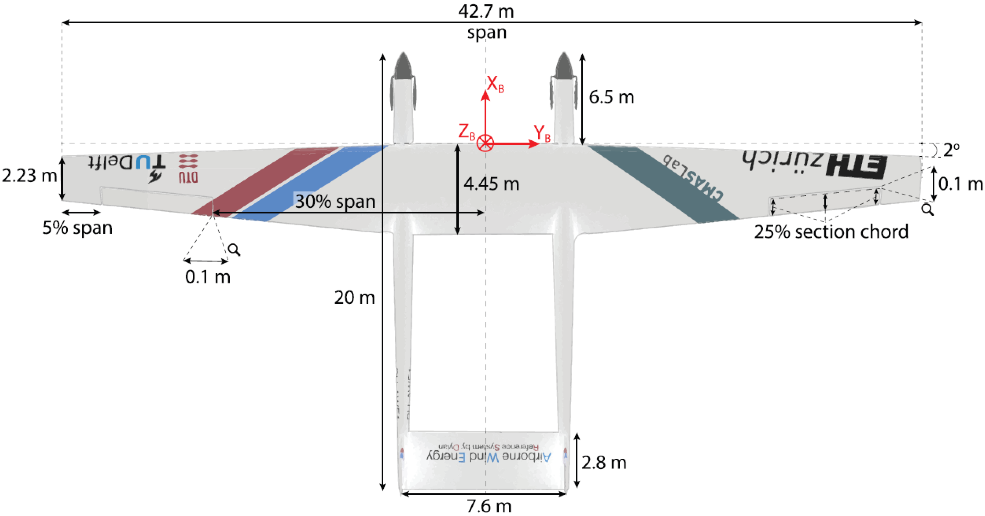
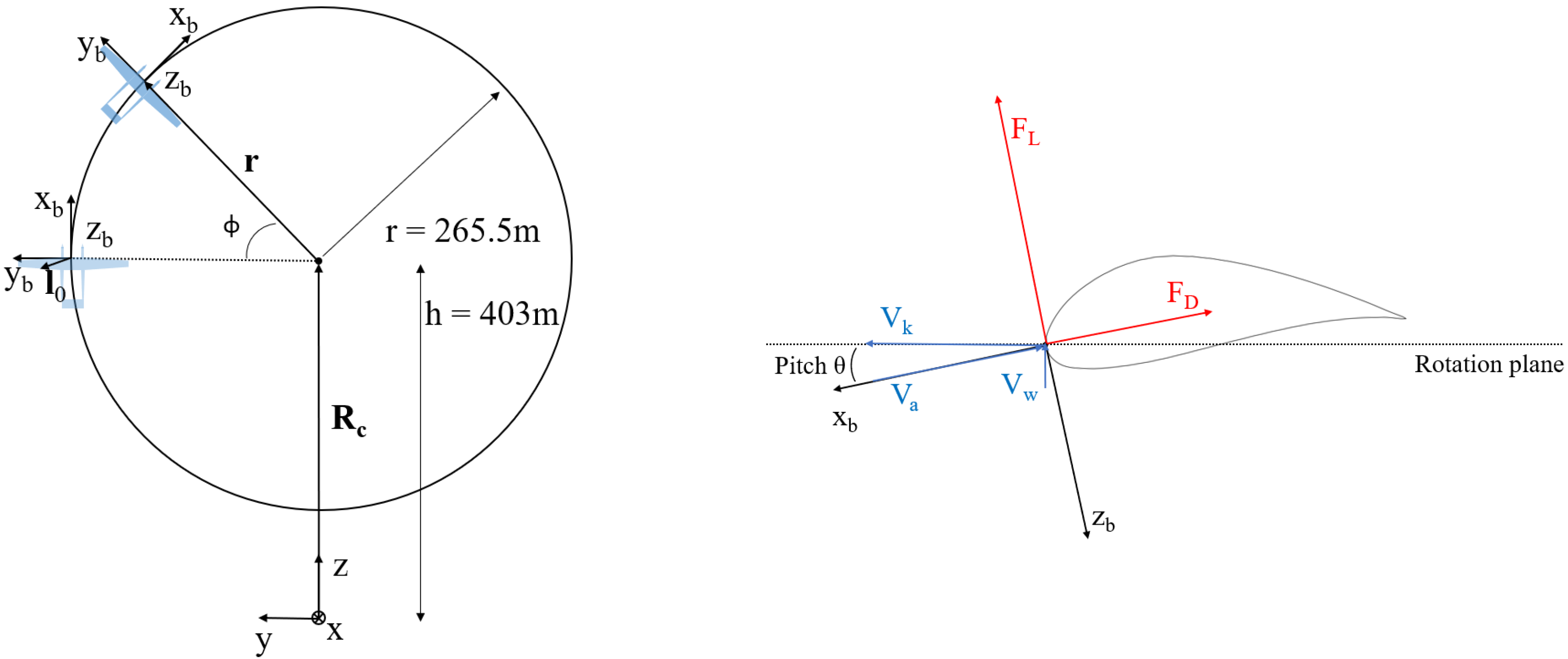
2.1. Aircraft Model and Flight Path
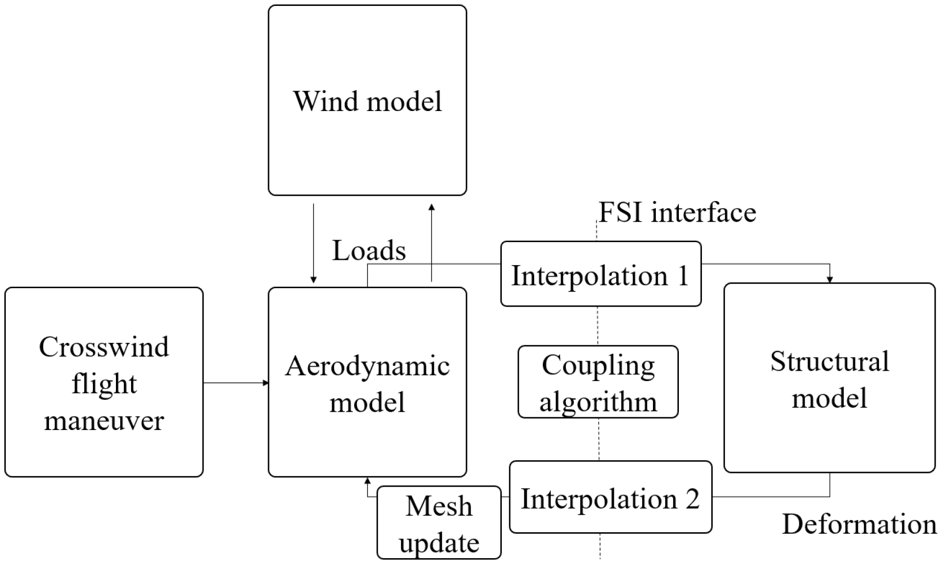
2.2. Fluid–Structure Interaction Framework
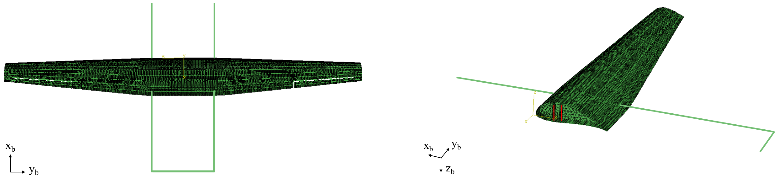
2.2.1. Structural Model
2.2.2. Aerodynamic Model
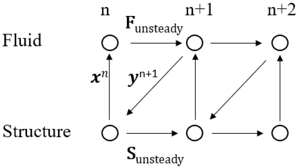
2.2.3. Interpolation and Coupling Algorithm
3. Results
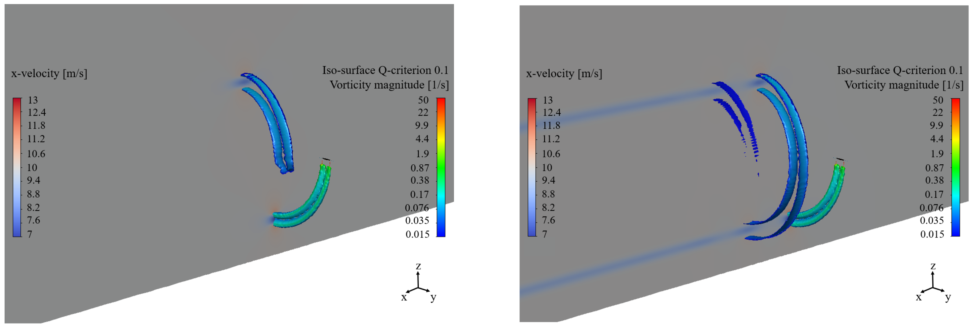
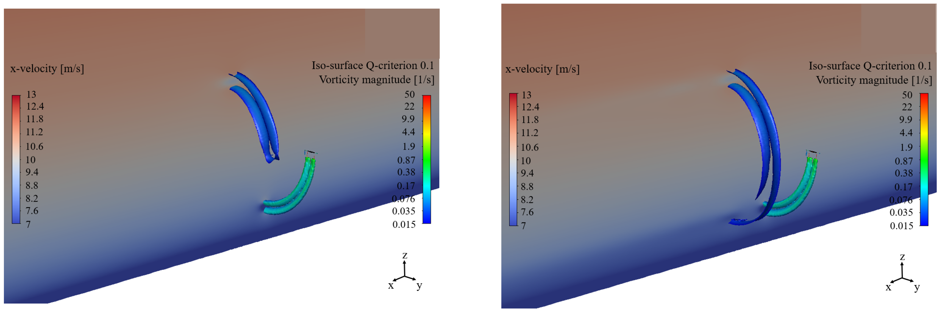
3.1. Unsteady Aerodynamics and Wake of a Starting AWE System
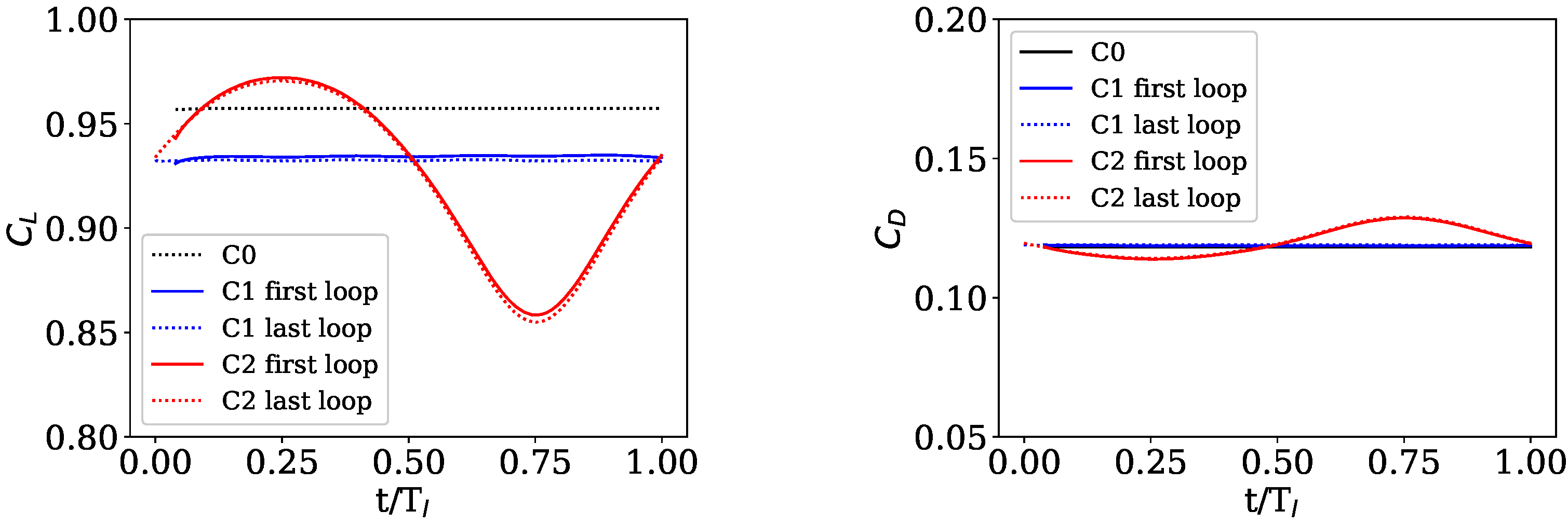
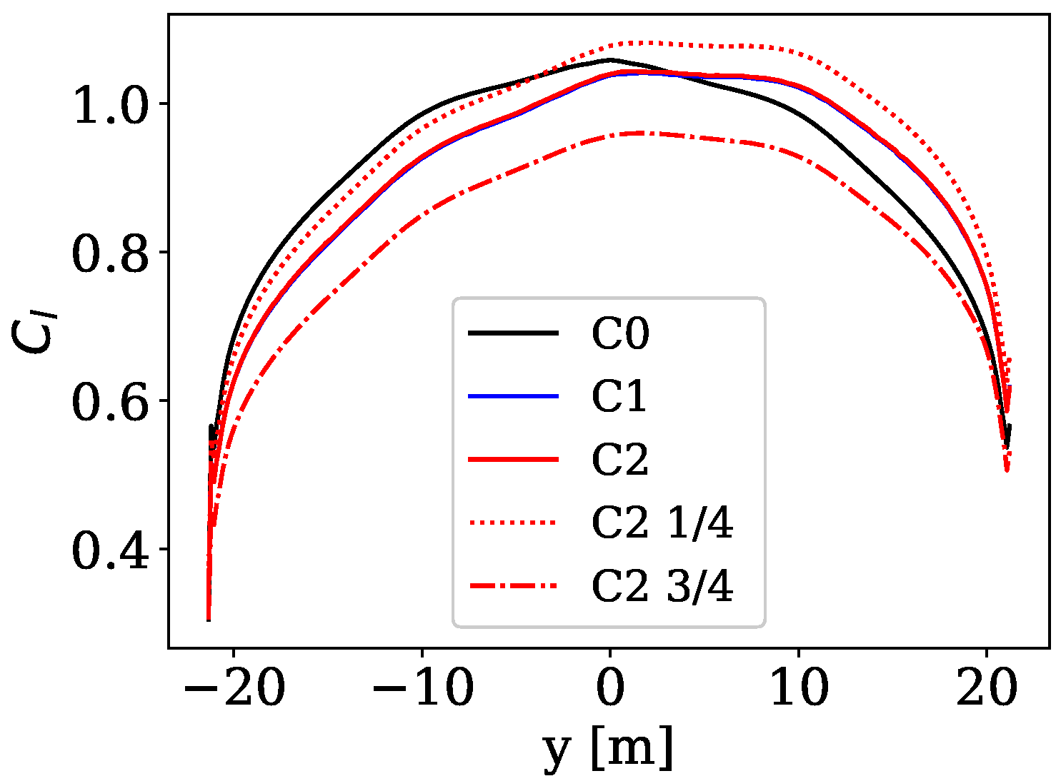
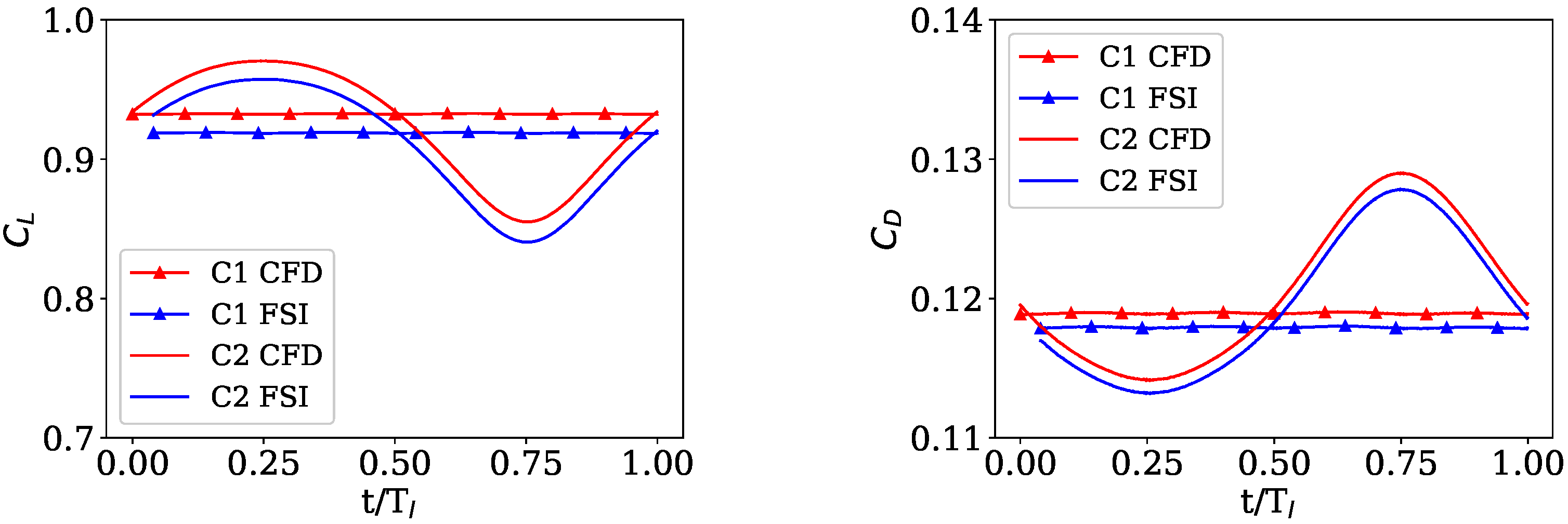
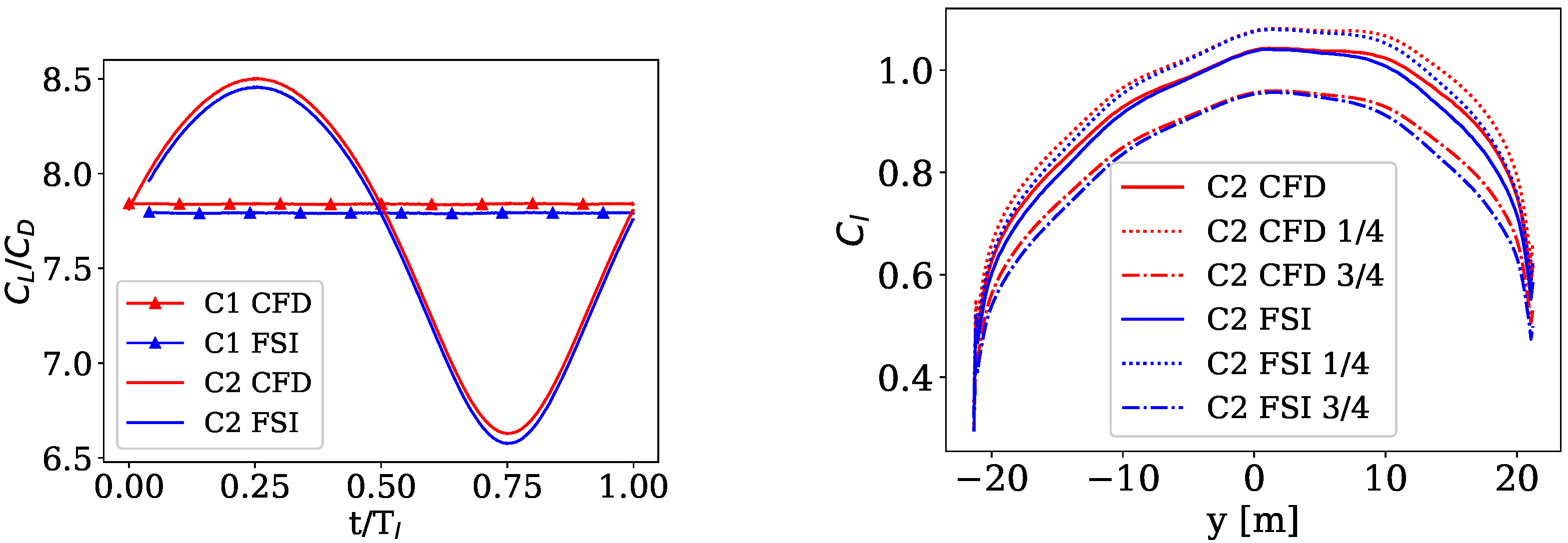
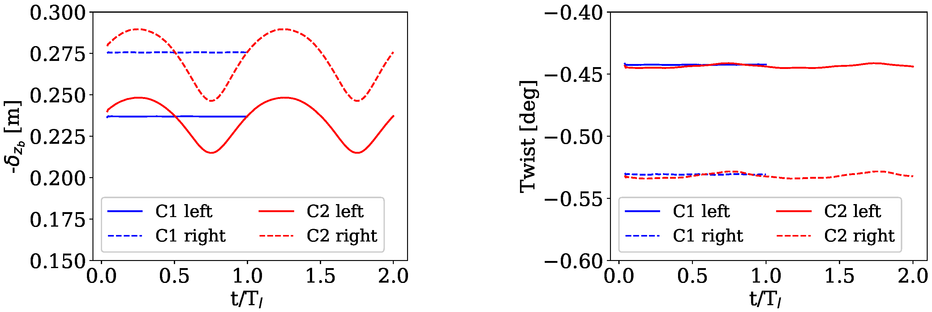
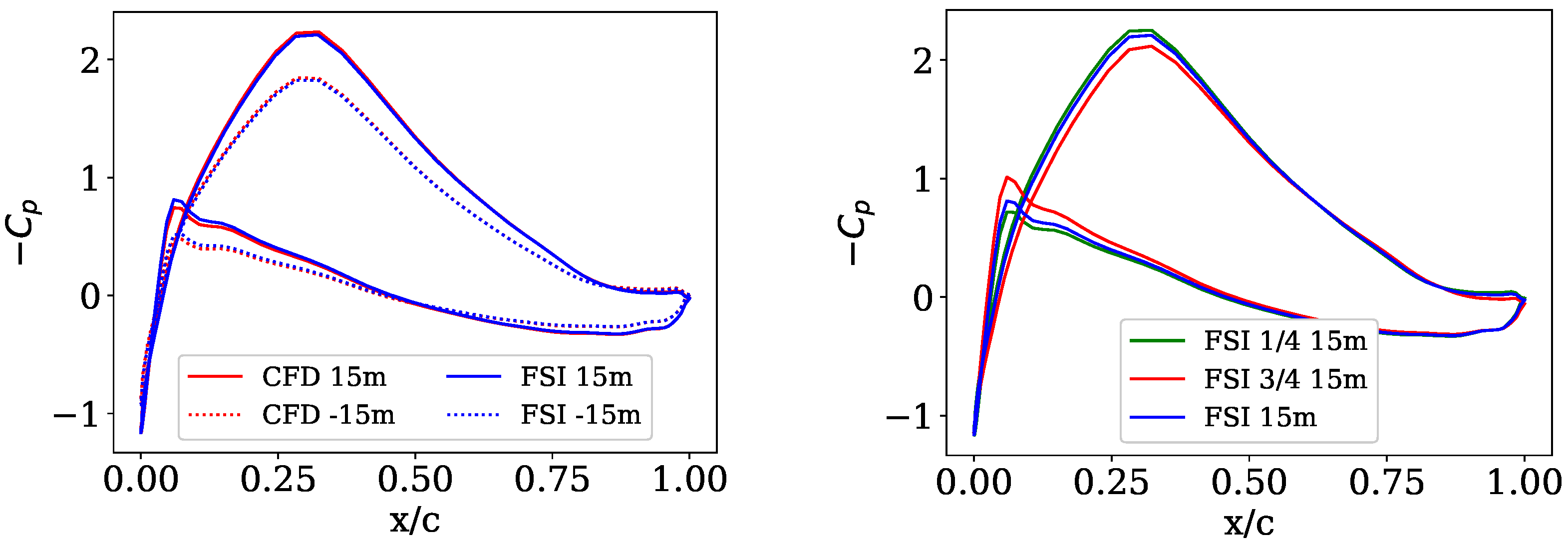
3.2. Crosswind Flight Simulations Including Fluid–Structure Interaction
3.3. Notes on Calculation Time
4. Conclusions and Outlook
Author Contributions
Funding
Data Availability Statement
Acknowledgments
Conflicts of Interest
Abbreviations
| ALE | Arbitrary Lagrangian–Eulerian |
| AWE | Airborne wind energy |
| B.c. | Boundary condition |
| BF | Bias factor |
| CFD | Computational fluid dynamics |
| CSM | Computational structural mechanics |
| FSI | Fluid–structure interaction |
| GR | Growth rate |
| N | Number of divisions |
| RANS | Reynolds averaged Navier–Stokes |
| SST | Shear stress transport |
| URANS | Unsteady Reynolds averaged Navier–Stokes |
| VSC | Flemish Supercomputer Center |
| 3DOF | Three degrees of freedom |
| 6DOF | Six degrees of freedom |
References
- Diehl, M. Airborne wind energy: Basic concepts and physical foundations. In Green Energy and Technology; Springer: Berlin/Heidelberg, Germany, 2014; pp. 3–22. [Google Scholar] [CrossRef]
- Echeverri, P.; Fricke, T.; Homsy, G.; Tucker, N. The Energy Kite: Selected Results from the Design, Development and Testing of Makani’s Airborne wind Turbines. 2020. Available online: https://x.company/projects/makani/ (accessed on 1 November 2022).
- Wijnja, J.; Schmehl, R.; Breuker, R.D.; Jensen, K.; Lind, D.V. Aeroelastic analysis of a large airborne wind turbine. J. Guid. Control Dyn. 2018, 41, 2374–2385. [Google Scholar] [CrossRef]
- Haas, T.; Schutter, J.D.; Diehl, M.; Meyers, J. Large-eddy simulation of airborne wind energy farms. Wind. Energy Sci. 2022, 7, 1093–1135. [Google Scholar] [CrossRef]
- Fasel, U.; Keidel, D.; Molinari, G.; Ermanni, P. Aeroservoelastic Optimization of Morphing Airborne Wind Energy Wings; AIAA SciTech Forum: San Diego, CA, USA, 2019. [Google Scholar] [CrossRef]
- Candade, A.A.; Ranneberg, M.; Schmehl, R. Aero-structural design of composite wings for airborne wind energy applications. J. Phys. Conf. Ser. 2020, 1618, 032016. [Google Scholar] [CrossRef]
- Eijkelhof, D. Design and Optimization Framework of a Multi-MW Airborne Wind Energy Reference System. Master’s Thesis, Delft University of Technology, Technical University of Denmark, Delft, The Netherlands, 2019. [Google Scholar]
- Castro-Fernández, I.; Borobia-Moreno, R.; Cavallaro, R.; Sánchez-Arriaga, G. Three-dimensional unsteady aerodynamic analysis of a rigid-framed delta kite applied to airborne wind energy. Energies 2021, 14, 8080. [Google Scholar] [CrossRef]
- Folkersma, M.; Schmehl, R.; Viré, A. Steady-state aeroelasticity of ram-air wing for airborne wind energy applications. J. Phys. Conf. Ser. 2020, 1618, 32018. [Google Scholar] [CrossRef]
- Viré, A.; Demkowicz, P.; Folkersma, M.; Roullier, A.; Schmehl, R. Reynolds-averaged Navier-Stokes simulations of the flow past a leading edge inflatable wing for airborne wind energy applications. J. Phys. Conf. Ser. 2020, 1618, 032007. [Google Scholar] [CrossRef]
- Vimalakanthan, K.; Caboni, M.; Schepers, J.G.; Pechenik, E.; Williams, P. Aerodynamic analysis of Ampyx’s airborne wind energy system. J. Phys. Conf. Ser. 2018, 1037, 062008. [Google Scholar] [CrossRef]
- Kheiri, M.; Victor, S.; Rangriz, S.; Karakouzian, M.M.; Bourgault, F. Aerodynamic performance and wake flow of crosswind kite power systems. Energies 2022, 15, 2449. [Google Scholar] [CrossRef]
- Hall, J. Aeroelastic Analysis of a Morphing Wing for Airborne Wind Energy Applications. Master’s Thesis, Lund University, Lund, Sweden, 2017. [Google Scholar]
- Kaufman-Martin, S.; Naclerrio, N.; May, P.; Luzzatto-Fegiz, P. An entrainment-based model for annular wakes, with applications to airborne wind energy. Wind Energy 2022, 25, 419–431. [Google Scholar] [CrossRef]
- Gaunaa, M.; Forsting, A.M.; Trevisi, F. An engineering model for the induction of crosswind kite power systems. J. Phys. Conf. Ser. 2020, 1618, 032010. [Google Scholar] [CrossRef]
- Eijkelhof, D.; Rapp, S.; Fasel, U.; Gaunaa, M.; Schmehl, R. Reference design and simulation framework of a multi-megawatt airborne wind energy system. J. Phys. Conf. Ser. 2020, 1618, 032020. [Google Scholar] [CrossRef]
- Eijkelhof, D.; Schmehl, R. Six-degrees-of-freedom simulation model for future multi-megawatt airborne wind energy systems. Renew. Energy 2022, 196, 137–150. [Google Scholar] [CrossRef]
- Vermillion, C.; Cobb, M.; Fagiano, L.; Leuthold, R.; Diehl, M.; Smith, R.S.; Wood, T.A.; Rapp, S.; Schmehl, R.; Olinger, D.; et al. Electricity in the air: Insights from two decades of advanced control research and experimental flight testing of airborne wind energy systems. Annu. Rev. Control 2021, 52, 330–357. [Google Scholar] [CrossRef]
- Santo, G.; Peeters, M.; Paepegem, W.V.; Degroote, J. Dynamic load and stress analysis of a large horizontal axis wind turbine using full scale fluid-structure interaction simulation. Renew. Energy 2019, 140, 212–226. [Google Scholar] [CrossRef]
- Grinderslev, C.; Horcas, S.H.; Sørensen, N.N. Fluid—Structure interaction simulations of a wind turbine rotor in complex flows, validated through field experiments. Wind Energy 2021, 24, 1426–1442. [Google Scholar] [CrossRef]
- Pynaert, N.; Wauters, J.; Crevecoeur, G.; Degroote, J. Unsteady aerodynamic simulations of a multi-megawatt airborne wind energy reference system using computational fluid dynamics. J. Phys. Conf. Ser. 2022, 2265, 042060. [Google Scholar] [CrossRef]
- Degroote, J.; Annerel, S.; Vierendeels, J. Stability analysis of Gauss-Seidel iterations in a partitioned simulation of fluid-structure interaction. Comput. Struct. 2010, 88, 263–271. [Google Scholar] [CrossRef][Green Version]
- Wieringa, J. Updating the davenport roughness classification. J. Wind. Eng. Ind. Aerodyn. 1992, 41, 357–368. [Google Scholar] [CrossRef]
- Parente, A.; Longo, R.; Ferrarotti, M. CFD boundary conditions, turbulence models and dispersion study for flows around obstacles. VKI Lect. Ser. 2017. [Google Scholar] [CrossRef]
- Yang, Y.; Gu, M.; Jin, X. New inflow boundary conditions for modeling the neutral equilibrium atmospheric boundary layer in SST k-ω model. J. Wind. Eng. Ind. Aerodyn. 2009, 97, 88–95. [Google Scholar] [CrossRef]
- Sorensen, J.; Shen, W. Numerical modeling of wind turbine wakes. J. Fluids Eng. 2002, 124, 393–399. [Google Scholar] [CrossRef]


| Field of Study | Low Fidelity | Mid-Fidelity | High Fidelity | |
|---|---|---|---|---|
| AWESs | Aero | S: [3,4] | S: [5,6,7], U: [8] | S: [9,10], U: [11,12] |
| Structure | [3] | [6] | [5,7,9] | |
| FSI | [3,5,7] | [6] | [9,13] | |
| Atmosphere | [12,14,15] | [4] (LES), [12] (RANS) | ||
| Dynamics | [8] | [4,16] | [5,17] | |
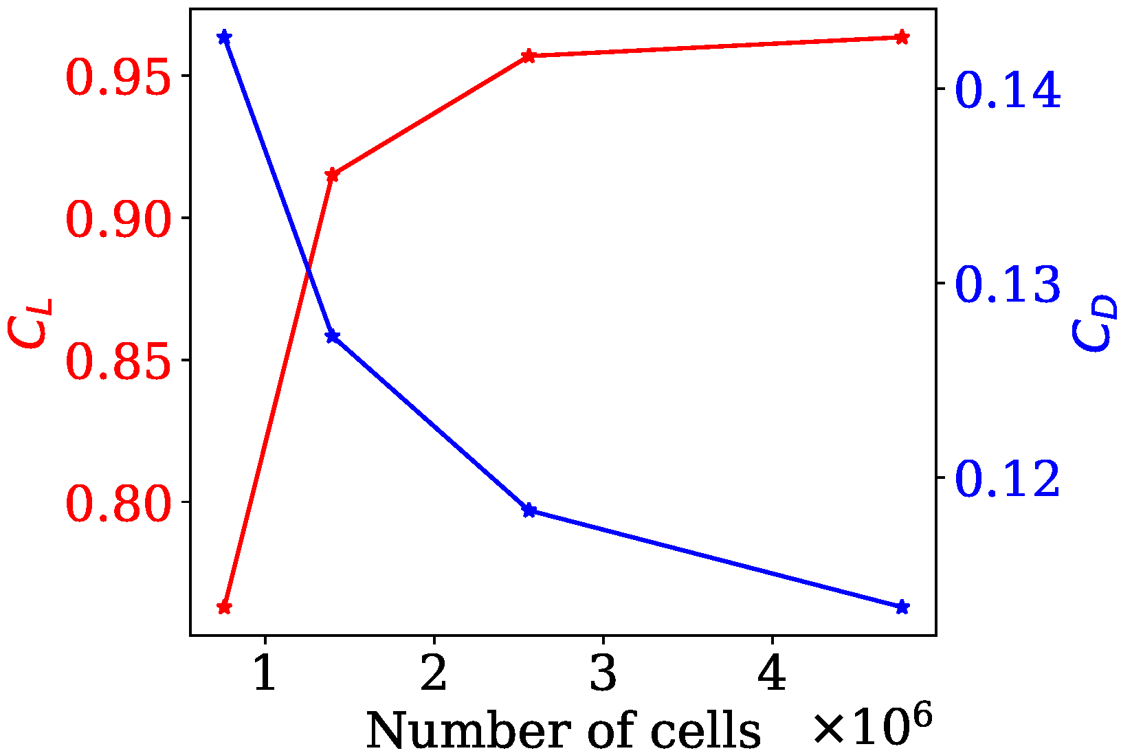
| Number of Cells | |
|---|---|
| Coarse | 0.76 × 10 |
| Medium | 1.40 × 10 |
| Fine | 2.56 × 10 |
| Ultra-fine | 4.76 × 10 |
| Configuration | Velocity Inlet () | Aircraft Speed () | Aircraft Pitch () |
|---|---|---|---|
| 0. Level flight | 0 m/s | 80 m/s | 0° |
| 1. Uniform wind | 10 m/s | 80 m/s | −7.125° |
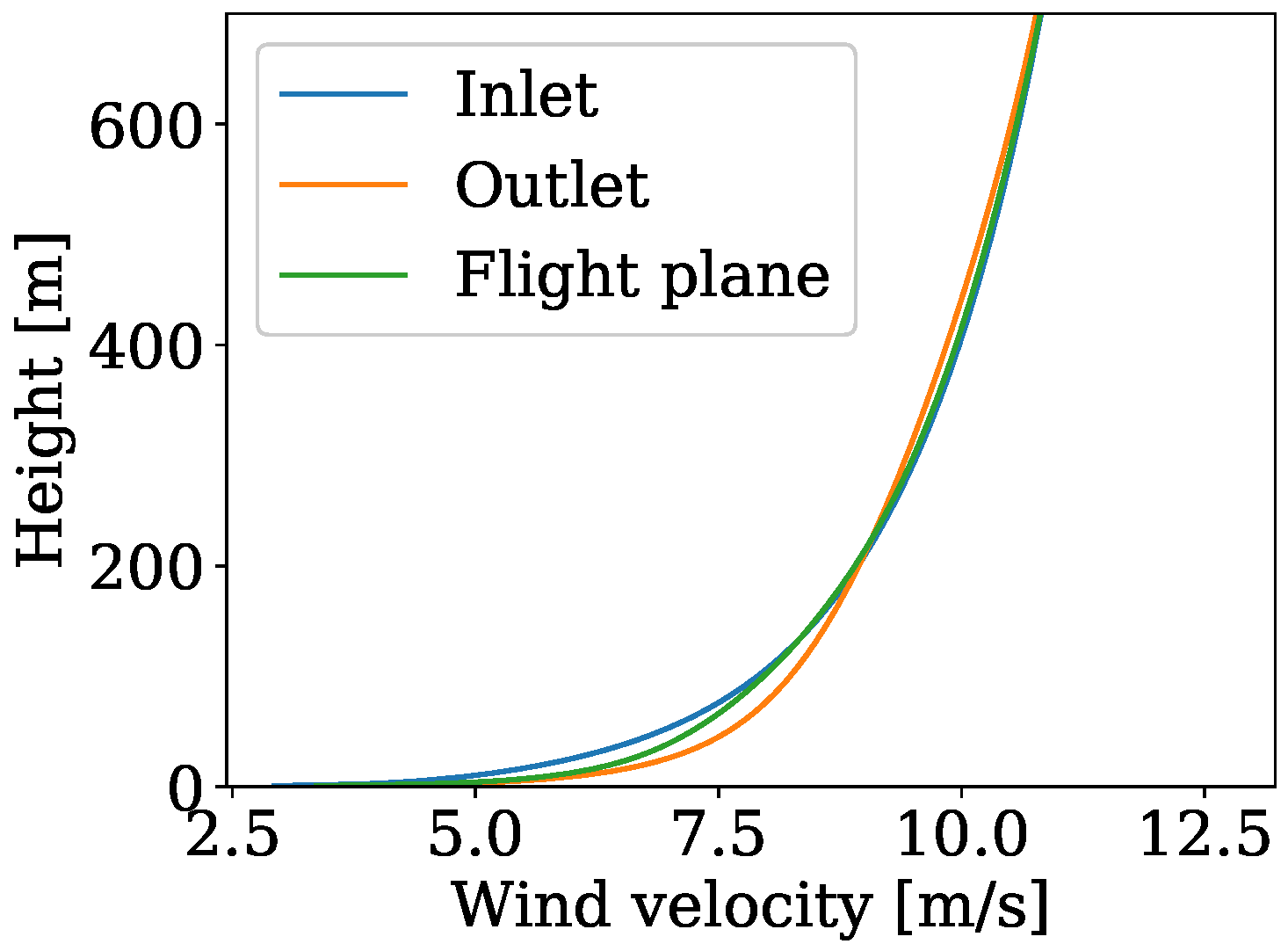
| 2. Logarithmic wind | Equation (1) | 80 m/s | −7.125° |
Disclaimer/Publisher’s Note: The statements, opinions and data contained in all publications are solely those of the individual author(s) and contributor(s) and not of MDPI and/or the editor(s). MDPI and/or the editor(s) disclaim responsibility for any injury to people or property resulting from any ideas, methods, instructions or products referred to in the content. |
© 2023 by the authors. Licensee MDPI, Basel, Switzerland. This article is an open access article distributed under the terms and conditions of the Creative Commons Attribution (CC BY) license (https://creativecommons.org/licenses/by/4.0/).
Share and Cite
Pynaert, N.; Haas, T.; Wauters, J.; Crevecoeur, G.; Degroote, J. Wing Deformation of an Airborne Wind Energy System in Crosswind Flight Using High-Fidelity Fluid–Structure Interaction. Energies 2023, 16, 602. https://doi.org/10.3390/en16020602
Pynaert N, Haas T, Wauters J, Crevecoeur G, Degroote J. Wing Deformation of an Airborne Wind Energy System in Crosswind Flight Using High-Fidelity Fluid–Structure Interaction. Energies. 2023; 16(2):602. https://doi.org/10.3390/en16020602
Chicago/Turabian StylePynaert, Niels, Thomas Haas, Jolan Wauters, Guillaume Crevecoeur, and Joris Degroote. 2023. "Wing Deformation of an Airborne Wind Energy System in Crosswind Flight Using High-Fidelity Fluid–Structure Interaction" Energies 16, no. 2: 602. https://doi.org/10.3390/en16020602
APA StylePynaert, N., Haas, T., Wauters, J., Crevecoeur, G., & Degroote, J. (2023). Wing Deformation of an Airborne Wind Energy System in Crosswind Flight Using High-Fidelity Fluid–Structure Interaction. Energies, 16(2), 602. https://doi.org/10.3390/en16020602