Unsteady Cloud Cavitation on a 2D Hydrofoil: Quasi-Periodic Loads and Phase-Averaged Flow Characteristics

Abstract

We perform large-eddy simulations to study a cavitating flow over a two-dimensional hydrofoil section—a scaled-down profile (1:13.26) of guide vanes of a Francis turbine—using the Schnerr–Sauer cavitation model with an adaptive mesh refinement in intensive phase transition flow areas. In the test case, the guide vane is tilted at an angle of attack of $9^{°}$ to the direction of the flow, in which the Reynolds number, based on the hydrofoil chord length, equals $1.32\times {10}^6$, thus providing a strong adverse pressure gradient along the surface. The calculated time-averaged turbulence characteristics are compared with those measured by particle image velocimetry to verify that the flow is correctly reproduced in numerical simulations using the procedure of conditional averaging proposed and tested in our previous investigation. A re-entrant jet is identified as the primary source of vapor cloud shedding, and a spectral analysis of the cavitating flow over the profile midsection is conducted. Two characteristic frequencies corresponding to the cases, when an attached cavity detaches completely (as a whole) and two partially from the hydrofoil, are found in the flow. The study reveals that the natural frequency of partial cavity shedding is three times higher than that of full detachments. The examined regime exhibits an oscillatory system with two oscillation zones related to cavitation surge instability and unsteady cloud cavitation resulting from the re-entrant jet. Conditional averaging correlates cavitation structures with pressure distributions, forces, and torque on the guide vane. This modeling approach captures the fine details of quasi-periodic cavitation dynamics, providing insights into unsteady sheet/cloud cavitation and offering a method for developing control strategies.

1. Introduction

Cavitating flow is a highly undesirable phenomenon in marine engineering and hydraulic systems as it negatively affects the operation and performance of machinery, causing enhanced noise, increased mechanical loads, and intensive material erosion [1,2,3,4]. A flow instability due to cavitation can also synchronise with vibrations of separate elements or the whole duct of a hydraulic unit, leading to their irreversible damage or failure. A comprehensive investigation of the spatial structure of partial cavities in connection with flow dynamics is complex. A detailed analysis of the physical mechanisms of cavitating flow unsteadiness is also one of the most important and urgent fundamental issues in the area of modern hydraulic engineering.

Unsteady partial cavitation is known to be accompanied by quasi-periodic oscillations of the length of the attached sheet cavity [5,6,7]. It is, admittedly, grouped into two main classes: unsteady sheet cavitation, i.e., the so-called cavitation surge, and unsteady cloud cavitation [8,9,10] with different origins. The cavitation surge is a system instability that prevails for quite long and thin cavities, typically of the length of 75–100% of a hydrofoil chord. No periodic detachments of large-scale cavitation clouds accompany this type of flow unsteadiness. The unsteady cloud cavitation, on the contrary, occurs for relatively short and thick cavities with the characteristic size of 40–60% of a chord length [8,10]. In this case, the source of instability is intrinsic, i.e., related to the cavity itself. Such a flow regime is characterized by the quasi-periodic shedding of large-scale cloud cavities, with the cavity length pulsations occurring at a frequency two-three times higher than for unsteady sheet cavitation conditions [7,11].

Two different mechanisms can govern the dynamics of unsteady cloud cavitation, namely the re-entrant jet and shock wave propagation. The re-entrant jet moves upstream underneath a sheet cavity due to an adverse pressure gradient along the surface of a test body [9,12,13]. If the pressure gradient is strong enough, it forces the re-entrant jet to impinge upon the cavity interface near its detachment line over the whole span or perimeter of the body. This process results in cutting off most of the vapor film. The separated part of the cavity then rolls up into a large-scale cavitation cloud due to the flow circulation appearing around it. Then, the formed cloud cavity is convected downstream by the primary flow, while the attached cavity starts to grow again. Next, an adverse pressure gradient along the surface forces the re-entrant jet to move upstream and this process repeats.

The shock wave propagation mechanism of unsteady cloud cavitation dominates, especially for gas-vapor cavities when cavitation represents a high-void-fraction bubbly mixture where the sound speed decreases approximately to the mean flow velocity or even lower [14,15]. In this case, a cloud cavity collapsing downstream produces a condensation shock that propagates upstream and pinches off a cavitation cloud, approaching the cavity detachment region. This occurs because the void fraction upstream of the shock front is significantly higher than the one downstream. As a result, the integrity of the attached cavity is disrupted and the gas–vapor mixture becomes discontinuous. It is worth noting that, despite the abundance of research on cavitation around generic symmetric foils [7,16,17,18,19], which even cover subtle spatial distributions of mean and turbulence characteristics, there remains a limited amount of comparative data for realistic shapes of machine and equipment elements, such as guide vanes and rotor blades. In particular, further investigations are required when the test body represents a foil shaped to replicate a 2D vane or a 3D blade, even in scaled-down models of real full-scale hydraulic machinery. This study focuses on the 2D scaled-down model of guide vanes featuring a symmetric cross-section. Our hypothesis revolves around the re-entrant jet being responsible for the unsteady behavior of cavitation, which will be demonstrated through investigation.

As shown in references [8,11,20], these different types of instabilities, namely system (a typical example being surge cavitation) and intrinsic instabilities (for example, unsteady cloud cavitation induced by the development of a re-entrant jet), are observed for symmetric two-dimensional bodies. Intrinsic instabilities are typically characterized by Strouhal numbers (St) ranging from 0.3 to 0.45, while system instabilities have St distributed between 0.05 and 0.2. As an illustration, Timoshevskiy M. et al. [11] have recently discovered asymmetric spanwise variations of an attached cavity length for unsteady flow conditions accompanied by alternating periodic cloud shedding from both sides of a hydrofoil. According to the numerical simulations by Decaix J. et al. [21], such an asymmetric cavity behavior is governed by the cross instability that is responsible for the existence of an oblique mode of cavity pulsations [22]. For these conditions, the oscillating system presumably falls into a bifurcation region between two zones of oscillations corresponding to the two main types of cavitation instabilities [7,10,20]. Thus, this regime is transient and the system eventually transits to one or another zone of stable pulsations. Regimes of this nature are relatively uncommon and present an intriguing area for exploration.

Recent experiments by Watanabe S. et al. [23] and Tsuru W. et al. [24] showed that cavitation inception and development significantly influence the hydrodynamic characteristics of a hydrofoil. At higher and moderate attack angles, while the attached cavity is stable, the lift force somewhat grows with cavitation evolution compared to the cavitation-free case. Once the flow regime transits to unsteady cloud cavitation, the time-averaged lift force slightly decreases but then increases again. Shed cloud cavities reaching the trailing edge of the hydrofoil reduce the lift force. When the partial cavity manifests unsteady sheet cavitation behavior (cavitation surge), the lift coefficient drastically drops, i.e., the so-called lift breakdown occurs. Experimental research by Keller A. [25] was conducted to examine the correlation between lift and drag coefficients and the cavitation number by testing various bodies. The experimental findings demonstrated a close relationship between the lift force and the inception of cavitation. The experiment by Watanabe S. et al. [23] mentioned above thoroughly investigated the connection between the mechanism of lift reduction and the unsteady behavior of a cavity around a two-dimensional Clark Y-11.7% hydrofoil. A detailed analysis of the instantaneous frequency spectra of the lift at various angles of attack was conducted, providing clarity on the relationship between these factors. This indicates that cavitation dynamics have a crucial impact on the magnitude of instantaneous values of the lift and are essential for the cavitation performance of a hydrofoil.

However, common cavitation models often appear to be incapable of the overall prediction of such important features of changes in the lift/drag force related to a cavitation pattern [26,27,28]. This shortcoming of numerical approaches is presumably explained by the presence of a high number of non-universal empirical flow parameters. Unsteady behavior of a cavitating flow may also be challenging for simulations [29,30]. Many successful studies employing numerical simulations of unsteady cavitation mainly focused on developing an effective modeling framework and on the analysis of various vorticity transport mechanisms to clarify the role of cavitation effects in the evolution of vortical structures [31,32,33,34,35,36,37]. Recently, the research emphasis has been on understanding the interconnection between the development of forces, energy transfer, and the dynamic behavior of cavitation, encompassing aspects such as cavity expansion, shedding, and collapse [38,39,40]. Therefore, in the realm of numerical modeling, a faithful replication of unsteady cavitation phenomena is crucial in assessing hydrofoil cavitation performance. This is essential for gaining insights into the underlying mechanism governing the interaction between forces and cavitation detachment. In this study, we make an attempt to overcome this difficulty, focusing on the evolution of a cavitating flow of a transient regime over a 2D hydrofoil at a moderate angle of attack (9°) and with high Reynolds numbers, with a special emphasis on the evaluation of quasi-periodic forces and conditionally averaged flow characteristics.

The paper is organized as follows. Section 2 provides the necessary details on the large-eddy simulation (LES) method. For a careful comparison of the numerical and experimental results, we describe and use the improved methodology based on the conditional averaging of velocity fields, which only considers data for the liquid phase [41]. Section 3 gives an analysis of the spatio-temporal evolution of cavitation structures together with the local flow dynamics based on the time-averaged flow velocity and turbulence characteristics. Also, the spectral characteristics are presented associated with the mechanism of the cavitation shedding process and lift-drag time history. Finally, we summarize our findings and make concluding remarks.

2. Modeling and Computational Details

We study a cavitating flow over a hydrofoil at a moderate angle of attack of 9° and a Reynolds number accompanied by sheet cavity detachment. The computational domain corresponds to our recent study [42] representing a $0.43$ m long channel with a rectangular cross-section of $0.08\times 0.25$ m${}^2$. A 2D symmetric profile resembling a scaled-down model of guide vanes of a Francis turbine to a scale of $1:13.26$ is considered. The chord length C is 100 mm and the aspect ratio is $L/C=0.8$, where $L=80$ mm is the foil span that is equivalent to the width of the test section (see Figure 1). The centerline of the rotating axis of the profile coincides with the geometric center of the hydrofoil. The investigated regime is characterized by two non-dimensional numbers, i.e., the Reynolds number $R{e}_C$ and cavitation number $\sigma$:

$$R{e}_C=\frac{{\rho }_l{U}_{0}C}{{\mu }_l},\sigma =\frac{p_0-p_v}{{\rho }_l{U}_0^2/2},$$

(1)

where ${\rho }_l$ and ${\mu }_l$ are the density and dynamic viscosity of the operating liquid (water), $U_0$ is the incoming flow velocity, $p_0$ is the reference static pressure at the test section sidewall measured at a distance of $7C=700$ mm upstream from the leading edge of the hydrofoil according to [42], and $p_v$ is the saturation vapor pressure of water (see

Table 1. Parameters of the flow regime considered in the present study.

${\mathit{U}}_0$ [m/s]	${\mathit{Re}}_{\mathit{C}}$ [-]	${\mathit{p}}_0$ [kPa]	${\mathit{p}}_{\mathbf{in}}$ [kPa]
$10.47$	$1.32\times {10}^6$	$105.8$	$85.3$
$\sigma$ [-]	${\rho }_l$ [kg/m${}^3$]	${\mu }_l$ [Pa×s]	$p_v$ [kPa]
$1.86$	$995.61$	$7.978\times {10}^{-4}$	$4.24$

). Subscripts l and v denote the liquid and vapor phase, respectively. At a water temperature of 30 °C, ${\rho }_l$ = $995.61$ kg/m${}^3$, ${\mu }_l=7.978\times {10}^{-4}$ Pa×s, and $p_v=4.24\times {10}^3$ Pa (see Table 1).

2.1. Governing Equations

The cavitating flow is described within the filtered Navier–Stokes equations using the volume-of-fluid (VOF) method as follows [43]:

$$\begin{array}{c}\hfill \frac{\partial \left(\tilde{\rho }{\widehat{u}}_i\right)}{\partial t}+\frac{\partial \left(\tilde{\rho }{\widehat{u}}_i{\widehat{u}}_j\right)}{\partial x_j}=-\frac{\partial \tilde{p}}{\partial x_i}+\frac{\partial {\widehat{\sigma }}_{ij}}{\partial x_j}-\frac{\partial {\widehat{\tau }}_{ij}}{\partial x_j},\end{array}$$

(2)

$$\begin{array}{c}\hfill \frac{\partial \tilde{\rho }}{\partial t}+\frac{\partial \left(\tilde{\rho }{\widehat{u}}_j\right)}{\partial x_j}=0,\end{array}$$

(3)

$$\begin{array}{c}\hfill \frac{\partial \left({\rho }_v\tilde{\alpha }\right)}{\partial t}+\frac{\partial \left({\rho }_v\tilde{\alpha }{\widehat{u}}_j\right)}{\partial x_j}=\tilde{R},\end{array}$$

(4)

where

$$\begin{array}{c}\hfill {\widehat{\sigma }}_{ij}=\tilde{\mu }\left(\frac{\partial {\widehat{u}}_i}{\partial x_j}+\frac{\partial {\widehat{u}}_j}{\partial x_i}-\frac{2}{3}{\delta }_{ij}\frac{\partial {\widehat{u}}_k}{\partial x_k}\right)\end{array}$$

(5)

is the viscous stress tensor and the term $\tilde{R}$ describes phase transitions. The tilde symbol denotes the spatially filtered fields while the hat symbol corresponds to the Favre-averaged quantity, i.e., ${\widehat{u}}_i=\widetilde{\rho u_i}/\tilde{\rho }$. The subgrid stresses term ${\widehat{\tau }}_{ij}$ is modeled using the dynamic k-equation subgrid-scale model [44]. Previously, we described in detail the modeling assumptions in Equations (2)–(4) (see reference [41]). The VOF framework considers $\tilde{\rho }$ and $\tilde{\mu }$ as follows:

$$\begin{array}{c}\hfill \tilde{\rho }=\tilde{\alpha }{\rho }_v+(1-\tilde{\alpha }){\rho }_l,\tilde{\mu }=\tilde{\alpha }{\mu }_v+(1-\tilde{\alpha }){\mu }_l,\end{array}$$

(6)

where subscripts l and v denote the liquid and vapor phase, respectively. The vapor volume fraction $\tilde{\alpha }$ varies from 0 for the liquid phase to 1 for the vapor.

To model phase transitions, the term $\tilde{R}$ is expressed using the Schnerr–Sauer model [45]:

$$\begin{array}{c}\hfill \tilde{R}=\frac{{\rho }_v{\rho }_l}{\tilde{\rho }}\tilde{\alpha }(1-\tilde{\alpha })\frac{3}{R_b}\mathrm{sign}(p_v-\tilde{p})\sqrt{\frac{3}{2}\frac{|p_v-\tilde{p}|}{{\rho }_l}},\end{array}$$

(7)

$$\begin{array}{c}\hfill R_b={\left(\frac{3}{4\pi }\frac{1}{n_0}\frac{\tilde{\alpha }}{1-\tilde{\alpha }}\right)}^{1/3},\end{array}$$

(8)

where $n_0$ is the empirical parameter corresponding to the bubble concentration per a unit volume of liquid. We set $n_0=1.6\times {10}^{13}$ according to the original publication.

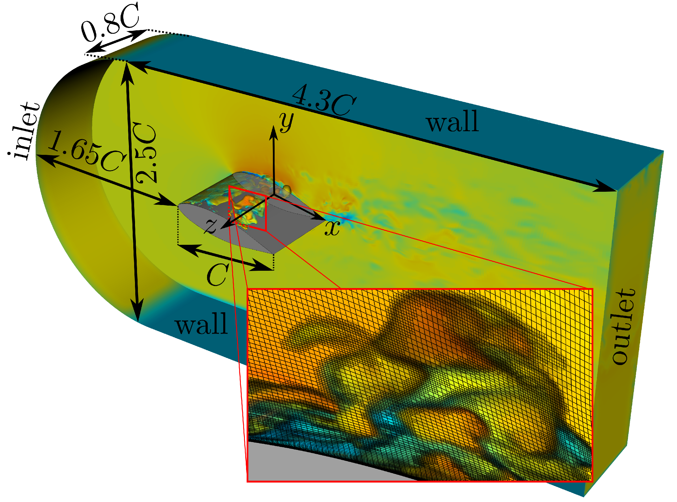
2.2. Numerical Details

The present numerical study was carried out using the computational code OpenFOAM [46]. The finite volume method (FVM) is used for the discretization of the governing equations which are solved using the $interPhaseChangeDyMFoam$ solver. For the spatial discretization of the diffusion terms in Equation (2), the second order central difference scheme is applied. The convection term is discretized using the second order accurate linear upwind differencing scheme [47]. The boundedness of the scalar field $\tilde{\alpha }$ is provided by the scheme proposed by reference [48] for the second term in Equation (4). For the time discretization, we use the Crank–Nicolson scheme [49]. The PISO scheme, consisting of a predictor and corrector steps, is used for the velocity-pressure coupling [50,51,52].

In simulations, we use unstructured computational mesh containing around $10.1\times {10}^6$ nodes. The number of computational nodes increases to $20\times {10}^6$ due to the dynamic mesh refinement procedure [53], see reference [41] for more details. Given that we are operating at a considerable distance from the Kolmogorov scale, indicating that our cell size is not sufficiently small to precisely depict the finest flow movement scales, the numerical methods employed to solve the discretized Navier–Stokes equations primarily possess a dispersive nature [54]. Consequently, the establishing of mesh convergence is conducted, and the details can be found in Appendix A. The inset in Figure 1 demonstrates the mesh refinement procedure where the hexagonal volumes are divided into eight subvolumes based on the local volume fraction of vapor in the range $0.4<\tilde{\alpha }<0.6$. On the walls, we set the no-slip boundary condition. The inflow velocity profile is set in agreement with the experiments [42], while the convective boundary condition is applied at the outflow. The inflow boundary conditions for the subgrid-scale kinetic energy $k_{sgs}$ and the volume vapor fraction $\tilde{\alpha }$ represent some fixed values close to zero. As for the pressure field, the Neumann conditions are specified at all boundaries, while the pressure at the inlet cross-section at a distance of $1.65C$ from the leading edge of the hydrofoil is set to $p_{in}$ by extrapolating the pressure value $p_0$ measured upstream [41]. To find $p_{in}$, we integrate the known velocity field from the experiment over the area of the inlet cross-section of the channel and get the change in pressure along the channel from the $p_0$ location to the inlet cross-section of the computational domain.

2.3. Experimental Apparatus and PIV Measurement

In this research, the experimental phase was conducted in the cavitation tunnel at the Institute of Thermophysics SB RAS, as described previously [55]. To observe the entire cavitating flow and analyze the integral characteristics of cavitation structures, a high-speed Photron FASTCAM SA5 camera was utilized. For measuring the planar velocity distributions around the hydrofoil, the PIV method was employed. Comprehensive information regarding the measurement instrumentation used for PIV implementation, processing, and validation procedures to assess velocity vector fields, as well as the evaluation of measurement uncertainties for different statistical characteristics, can be found in our recent study [42]. In the same study, the measurement error of quantification of instantaneous flow velocity, which is mainly caused by uncertainties in the cross-correlation processing employed in the PIV method, was assessed. It was shown that its typical value does not exceed 0.1 pixel for a $32\times 32$ pixel interrogation area, which corresponds to relative errors of $\delta U=1\%$ and $4\%$ for particle displacements of 8 and 2 pixels, respectively (see details in reference [55]). As the uncertainty in measuring turbulence properties is significantly dependent on the statistical volume used for their calculation, the effect of sample size was also considered in reference [55] and further analyzed in reference [42] for the mean velocity, Reynolds stresses, and turbulent kinetic energy. According to reference [55], to calculate both the time-averaged velocity and second-order moments of turbulent fluctuations in cavitating flow, it is well sufficient to have 1500 instantaneous realizations. However, it is not enough for the precise evaluation of higher-order statistical moments. Nevertheless, the higher-order moments can be estimated with high confidence based on a statistic of 1700 realizations, provided that the procedure of statistical vector filtration is used (see details in reference [56]).

3. Results

In our previous paper, we proposed a methodology for the direct comparison of PIV and LES data based on the conditional averaging of velocity fields for certain values of $\tilde{\alpha }$ given that the experimental results contain information on the liquid phase only [41]. The conditional averaging of velocity fields is defined as:

$$\begin{array}{c}\hfill {\langle {\widehat{u}}_i\rangle }_{{\tilde{\alpha }}_{th}}=\langle {\widehat{u}}_i|\tilde{\alpha }<{\tilde{\alpha }}_{th}\rangle ,\end{array}$$

(9)

where the averaging procedure $\langle .\rangle$ is only performed for samples with $\tilde{\alpha }<{\tilde{\alpha }}_{th}$ in the same spatial position, where ${\tilde{\alpha }}_{th}$ is a threshold. Below, we employ the value ${\tilde{\alpha }}_{th}=0.25$ to compare the PIV and LES results.

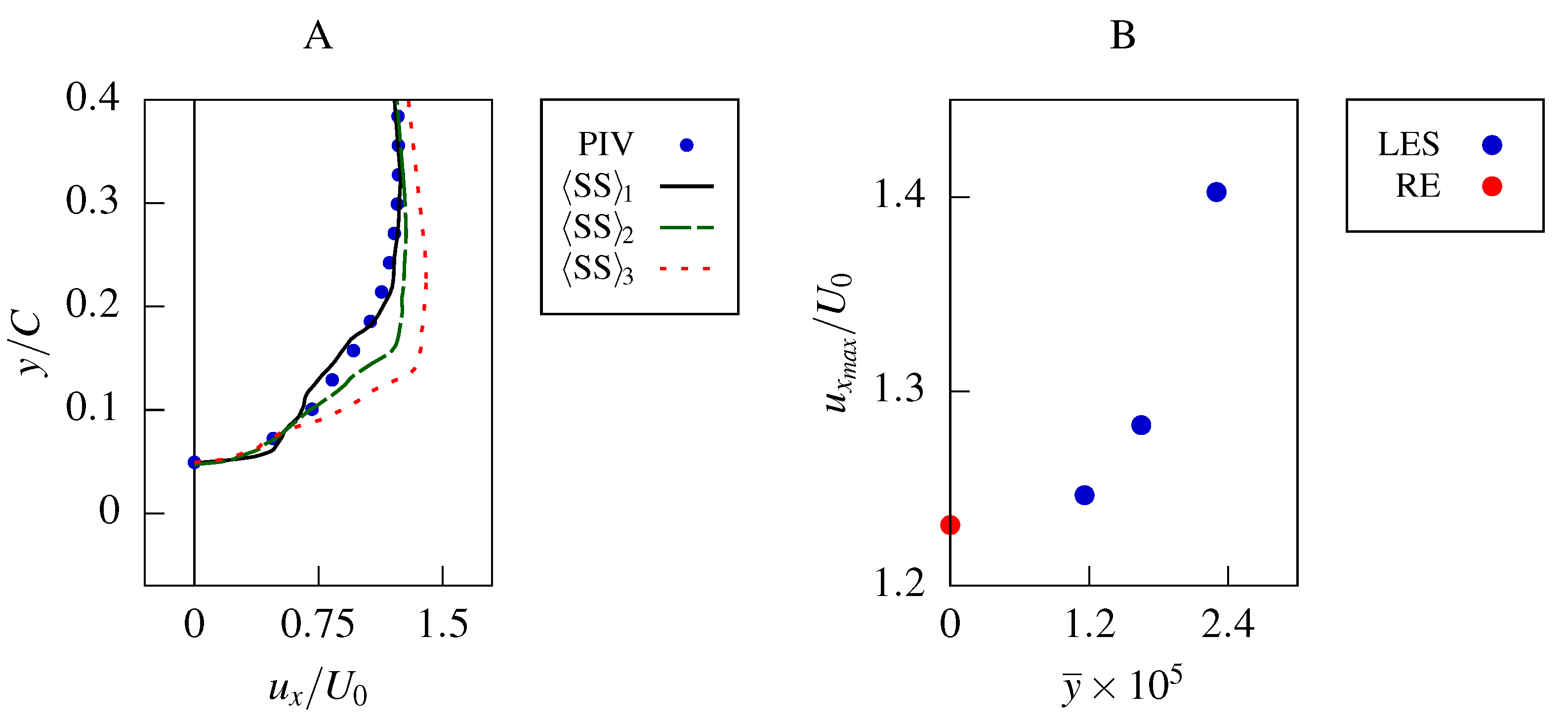
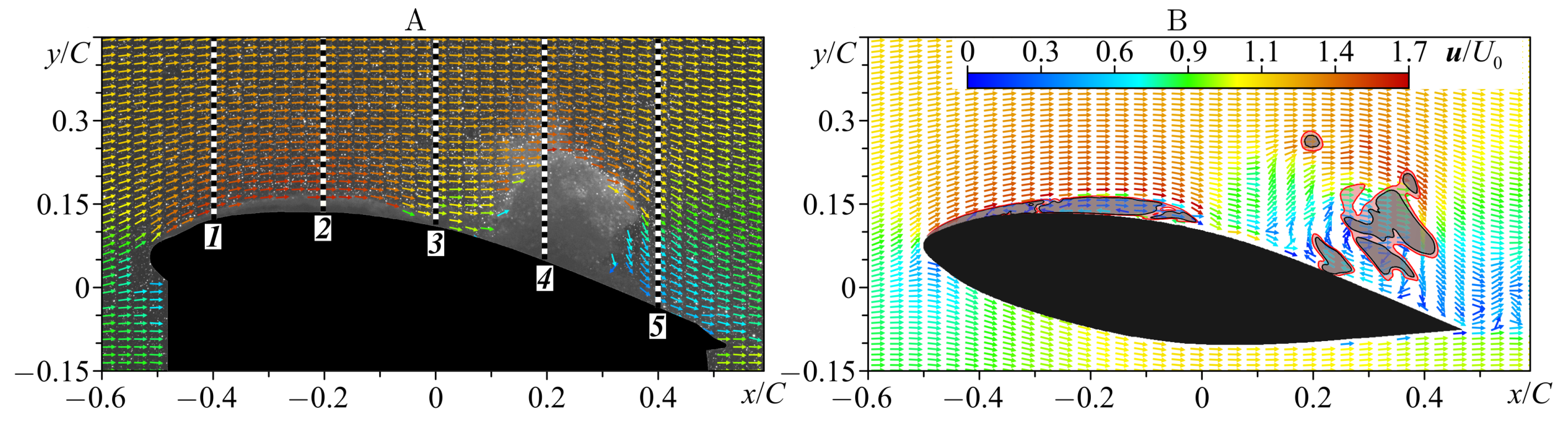
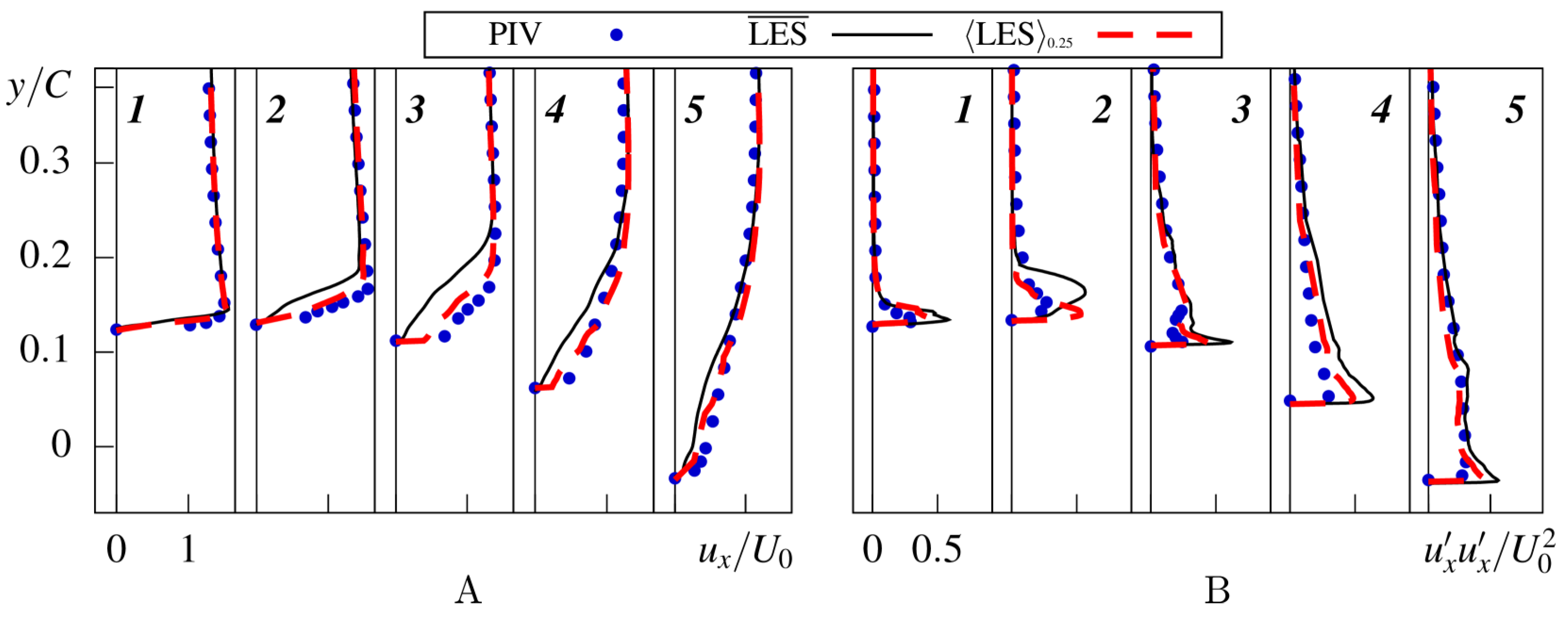
3.1. Comparison with Experiments

Figure 2 qualitatively compares the PIV [11] and LES velocity fields in a similar phase of the cloud shedding process. A good agreement in the size and position of the attached cavity can be observed. Compared to the experimental data, LES gives information in the regions that the cavity occurs (see Figure 2). In order to compare the time-averaged velocity and its fluctuations profiles, we use the conditional averaging procedure described above (see Equation (9)). As seen in Figure 3, the PIV and LES results are in excellent agreement for cross-section 1 and closely match one another in position 2. Small discrepancies between the numerical and experimental velocity profiles are observed in positions 3 and 4 due to the fact that cavitation is basically present in the middle part of the hydrofoil. For position 5, low-frequency passages of cloud cavities in this region do not contribute significantly to the evaluation of the statistical characteristics, which results in very tiny dissimilarities of the profiles of both quantities shown in Figure 3. The overall results of the PIV and LES showed that the proposed methods are relevant.

3.2. Lift/Drag Force Coefficients and Conditional Averaged Characteristics

The unsteady cavitation behavior apparently causes changes in the lift and drag forces acting on the hydrofoil. To analyse these forces, we use lift and drag coefficients, which are defined as follows:

$$\begin{array}{c}\hfill C_L=\frac{lift}{0.5{\rho }_l{U}_0^{2}S},C_D=\frac{drag}{0.5{\rho }_l{U}_0^{2}S},\end{array}$$

(10)

where L and D correspond to the lift and drag forces, respectively, and S is the hydrofoil surface area. We neglect the friction force due to its insignificant contribution at large Reynolds numbers. Figure 4A shows a typical time history of $C_L$ and $C_D$. Both $C_L$ and $C_D$ oscillate periodically, with their amplitudes ranging from $0.21$ to $0.84$ (${\overline{C}}_L=0.53$) and from $0.02$ to $0.14$ (${\overline{C}}_D=0.08$), respectively, where the overline denotes time-averaging. The general trend of $C_L$ and $C_D$ is that both curves grow slowly from valley $t_1$ to trough $t_4$ (Figure 4B), then the curves decline rapidly from the peak to the end of the first cycle $t_1^{*}$ (see Figure 4B). The oscillatory behaviour of these coefficients is phase-shifted on $\Delta$ value (see Figure 4B).

Let us consider one period of oscillations of both coefficients, indicated in Figure 4B as $t_1-t_1^{*}$, in more detail. Figure 5 shows the whole cavitation shedding process, which begins with stage $t_1$ (Figure 4A). The length of the attached cavity $L_C$ starts to increase and eventually reaches $1/4$ of the chord, and $C_L$ is minimal at this moment. The small region with a negative velocity is observed in the part of the hydrofoil closest to the leading edge, indicating the possible formation of a re-entrant jet. In Figure 5C($t_1$–$t_1^{*}$), the Q-criterion is used for representing the flow vortex structure. It is visible that vortices generated from the midchord to the trailing edge of the hydrofoil are approximately the same size. At stage $t_2$, $C_L$ takes the value between its minimum and zero (Figure 4B) and corresponds to the moment when a cloud cavity detaches from the cavitation sheet (Figure 5A($t_2$),B($t_2$),C($t_2$)). This occurs due to the upstream movement of a re-entrant jet, which develops underneath the attached cavity as a result of an adverse pressure gradient, leading to the cavity interface breakdown (see Figure 5B($t_2$)). The shedding of the formed cloud cavity leads to a slight increase in the size of the vortical structures in this region. This cloud cavity is advected downstream by the primary flow to the trailing edge, where a backflow induced in the aft part of the hydrofoil turns into the re-entrant jet. This leads to the detachment of the next cloud cavity (see Figure 5A($t_3$),B($t_3$),C($t_3$)). The second cloud cavity hovers over the trailing edge and the vertical structures in the region grow in size. In contrast to the previous stage, stage $t_4$ is characterized by an intensive re-entrant jet on the foil. Stage $t_4$ corresponds to the maximum value of $C_L$ and precedes the moment of the third shedding of the cavitation cloud (see Figure 5A($t_4$),B($t_4$),C($t_4$)). Similarly to stage $t_4$, at stage $t_5$, the detached cloud cavity moves downstream along the surface of the hydrofoil, leading to a decrease in $C_L$ and an increase in the cavitation structures behind the trailing edge. Next, at stage $t_1^{*}$, the size of the vortex structures is decreased in a similar way as for stage $t_1$, the formation of a new re-entrant jet begins again in the nose part of the hydrofoil, and then the process of cloud cavitation shedding repeats.

The lift force coefficient $C_L$ acting on the upper and lower surfaces of the foil was considered separately. The evolution of the absolute values of $C_{L_{up}}$ and $C_{L_{down}}$ is shown in Figure 6A. The curve’s behavior undergoes a change at the characteristic time points $t_1-t_1^{*}$, indicating either a detachment of the cloud cavity ($t_2$,$t_3$ and $t_5$) or the minimum and maximum presence of cavitation on the hydrofoil surface. Based on the values of $C_L$, we perform conditional averaging of the fields of velocity, pressure, and vapor volume fraction $\alpha$. The conditional averaging was carried out for four characteristic times $t_1-t_1^{*}$ (see Figure 7). When the extent of the attached cavity $L_C$ on the hydrofoil surface is shortest (Figure 7C($t_1$)), the flow velocity in the nose part is much higher that at other times (see Figure 7A($t_1$)). Meanwhile, in the aft part of the model, the flow is slowed down (see Figure 7A($t_1$)). Also, the pressure is very low only in the first half of the upper part of the foil in Figure 7B($t_1$). An increase in the cavitation area on the foil surface corresponds to characteristic time $t_2$ (see Figure 7C($t_3$)). The low-pressure region increases in the streamwise direction from the leading edge to the hydrofoil midsection (see Figure 7B($t_3$)). In this region, a zone of decelerated flow also appears but, near the trailing edge, the flow speeds up again (see Figure 7A($t_3$)). At the characteristic time $t_4$ the largest amount of vapor is located on the surface of the foil (see Figure 7C($t_4$)). The flow decelerates from the leading edge to the trailing one (see Figure 7A($t_4$)). As for the pressure, the low-pressure region is the largest of all considered cases. A further decrease in the $L_C$ corresponds to time $t_5$ (see Figure 7C($t_5$)). The region of reduced velocities, in turn, shifts closer to the trailing edge (see Figure 7A($t_5$)), where the pressure increases (see Figure 7B($t_5$)).

3.3. Spectral Characteristics

We carried out the analysis of the cavitating flow dynamics based on the numerical data using the experimental images [42]. Image processing was performed along the red dashed line (cross-section $x=-0.05C$) in Figure 8A. Each pixel on this line has its own intensity $i\left(z\right)$, which varies in the range between 0 (absolutely black) to 255 (purely white). The mean value of $i(z,n)$ over the time $\left(n\right)$ is given by the following:

$$\begin{array}{c}\hfill i\left(z\right)=\frac{1}{N}{\displaystyle \sum _{n=1}^N}i(z,n),\end{array}$$

(11)

where N is the number of images corresponding to full experimental statistics, $i(z,n)$ is the level of intensity of the pixel with coordinate z, and time moment n. The normalized values $I\left(z\right)=i\left(z\right)/255$ are averaged in a spanwise direction:

$$\begin{array}{c}\hfill I_z=\frac{1}{n_z}{\displaystyle \sum _{k=1}^{n_z}}I\left(z_k\right),\end{array}$$

(12)

A similar procedure was applied to the vapor volume fraction $\alpha$ obtained in LES. The numerical simulation data were averaged in the x-direction (within range of $-0.175C<x<0.175C$) and y-direction ($0.05C<y<0.25C$). For further analysis of the cavity dynamics, we conducted the Fourier transform of $I_z$ and ${\alpha }_z$ averaged over time and in the spanwise direction to obtain the dominant frequencies of cloud shedding. Its results, in arbitrary units (a.u.), are shown in Figure 8B as a function of nondenominational frequency (Strouhal number) St $=f{L}_C^{max}/U_0$, where f is the cavity shedding frequency and $L_C^{max}=0.56C$ is the maximum streamwise dimension of an attached cavity. Low frequencies are well reproduced by LES, which shows the dominant frequency to be St${}_{LES}\approx 0.112$ which is very close to St${}_{Exp}\approx 0.106$. Figure 8B also demonstrates that there is a second maximum in the spectrum. It is observed at higher frequencies St${}_{LES}\approx 0.33$, which is slightly lower than the one in the experiment St${}_{Exp}\approx 0.34$. Despite insignificant differences, LES appears to be capable of predicting the dynamics of the cavitating flow quite well. Figure 8C shows time evolution of instantaneous vapor volume fraction ${\alpha }_z$ averaged over the hydrofoil span, indicating the presence of the two frequencies in the spectrum in Figure 8B. As shown in Figure 5, one shedding cycle involves three cloud detachments, which is also clearly seen in Figure 8C. Accordingly, the frequency of the higher harmonic with St${}_{LES}\approx 0.33$ is three times larger than that of the dominant one (St${}_{LES}\approx 0.112$) and corresponds to a partial detachment of cloud cavities.

The presence of two peaks in the frequency spectrum indicates the existence of two types of instabilities in the flow. Lower Strouhal number zones correspond to cavitation surge instability and higher St unsteady cloud cavitation, respectively. Based on the previous investigations [7,20], the fact that the maximum length of the attached cavity reaches $L_C^{max}=0.56C$ indicates that unsteady cloud cavitation, induced by the presence of a re-entrant jet, is the primary instability observed in our case.

4. Conclusions

Large-eddy simulations of an unsteady cavitating flow around a two-dimensional hydrofoil mimicking a guide vane of a Francis turbine to a scale of 1:13.26 were performed at an angle of attack of $9^{°}$ and a high Reynolds number of $R{e}_C=1.32\times {10}^6$. We used a finite-volume method, coupled with a dynamic mesh refinement procedure, to increase the calculation accuracy in the flow regions where intensive phase transitions occur. To simulate cavitation, we employed the Schnerr–Sauer model. To properly reproduce quasi-periodic behavior of the unsteady cavitating flow, numerical results were conditionally averaged, thus allowing the phase-by-phase tracking of the time evolution of cavitation structures and associated flow structures. Such a modeling approach, combined with phase averaging, made it possible to accurately validate the LES results against those measured by PIV [11], showing excellent overall agreement between both datasets by the example of spatial distributions of the conditionally averaged flow velocity and its fluctuations. A comparative analysis of natural frequencies of cloud cavity shedding, obtained numerically and experimentally through visual observations, also demonstrated the high precision and reliability of the modelling technique. Although the models under investigation did not take into account the compressibility effect, they still showed good agreement with the experimental data. This serves as a starting point for further research on the impact of second mechanism governing the dynamics of unsteady cloud cavitation, as discussed in reference [19].

Thanks to this upgraded simulation technology, the global dynamics of the vapor cloud shedding process was reviewed and described in more detail compared to the available literature. The presence of vapor cavities in the flow was proven to cause an increase in the size of large-scale vortical structures. Additionally, we demonstrated that the re-entrant jet mechanism is typical for this regime, supported by its presence underneath the attached cavity and the satisfactory agreement between the velocity and fluctuation fields from the LES and experimental data. It was found that typical cavitation sheet auto-oscillations are characterized by two dominant frequencies, where one is three times higher than the other, thus being a higher harmonic of the latter. These two frequencies are, respectively, attributed to two partial (a sheet cavity remains partially attached to the hydrofoil after its interface breakup) and complete (a sheet cavity separates completely as a whole) detachments of attached cavities, followed by the formation of cloud cavities. Given that the current flow regime is transitional, we may assume that cavitation surge instability contributes to the formation of the re-entrant jet, leading to an intensified adverse pressure gradient along the foil surface, consequently causing the observed cloud cavity detachment. Moreover, it is probable that the presence and concurrent development of cavitation surge instability suppress the mechanism of shock wave propagation, as both phenomena are influenced by changes in the pressure field. The presence of cavitation was correlated with pressure fields of the flow as well as the magnitude of the resultant force acting on the hydrofoil, based on appropriate conditionally averaged results for the selected time instants. Taking the time history of the lift $C_L$ and drag $C_D$ coefficients into account, this force was shown to have the greatest effect when the largest amount of vapor phase is present over the guide vane, accordingly slowing down the flow in that region, and vice versa. When $C_L$ decreases during a growth/reduction cycle of cavitation, the length of an attached cavity decreases along with the overall vapor fraction, while the flow, on the contrary, accelerates. Thus, the numerical approach employing the LES and the Schnerr–Sauer model to simulate turbulence and cavitation, respectively, combined with the procedure of conditional averaging, was shown to be capable of capturing the minute details of the quasi-periodic dynamics of cavitation structures, gaining important information on the fine features inherent to the cavitating flow, which could not be obtained otherwise:

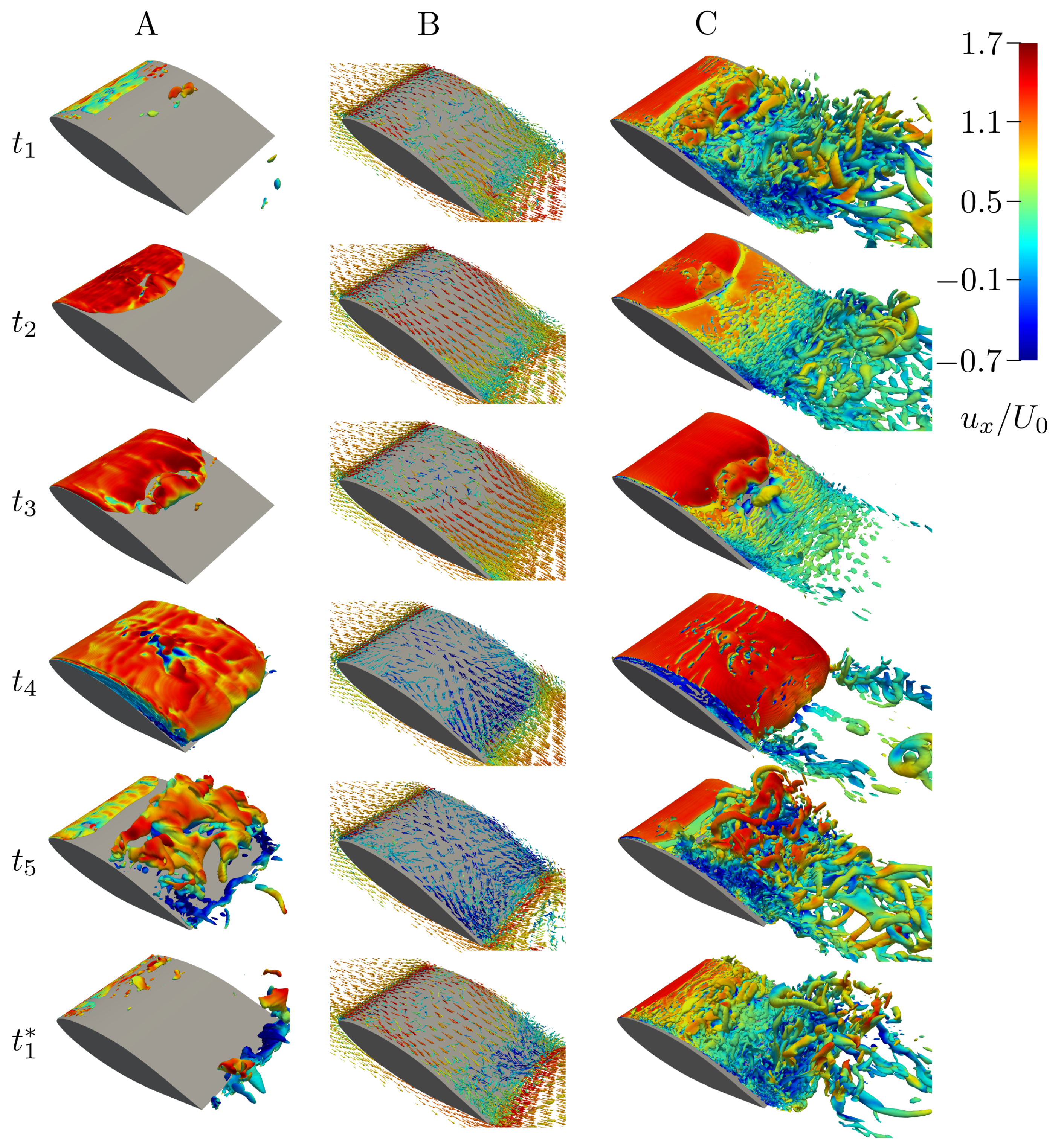
• The simulations revealed the presence of vapor cavities leading to an increase in large-scale vortical structures and the occurrence of a re-entrant jet mechanism;
• Two dominant frequencies in cavitation sheet auto-oscillations were identified, and their interaction with cavitation surge instability was explored;
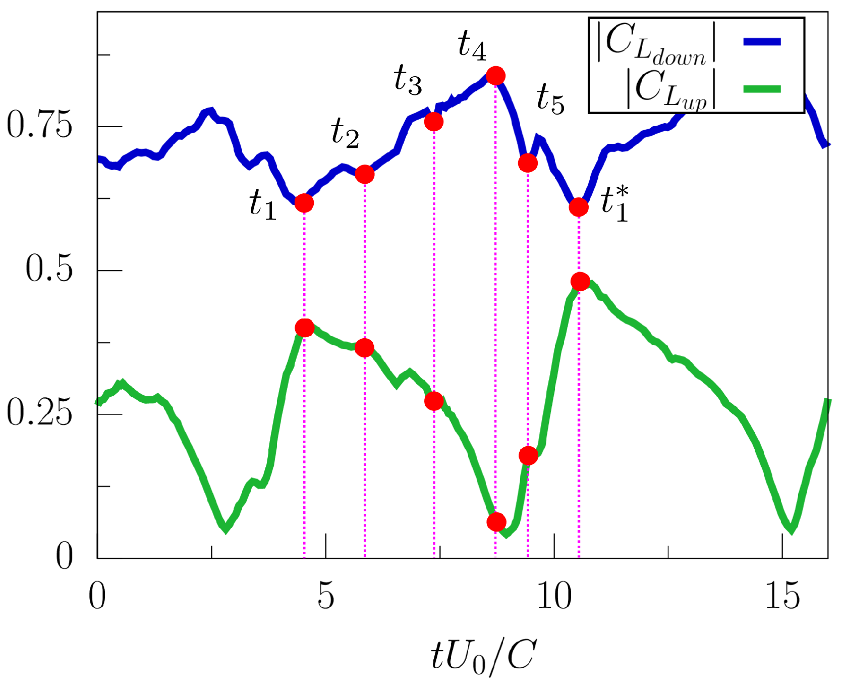
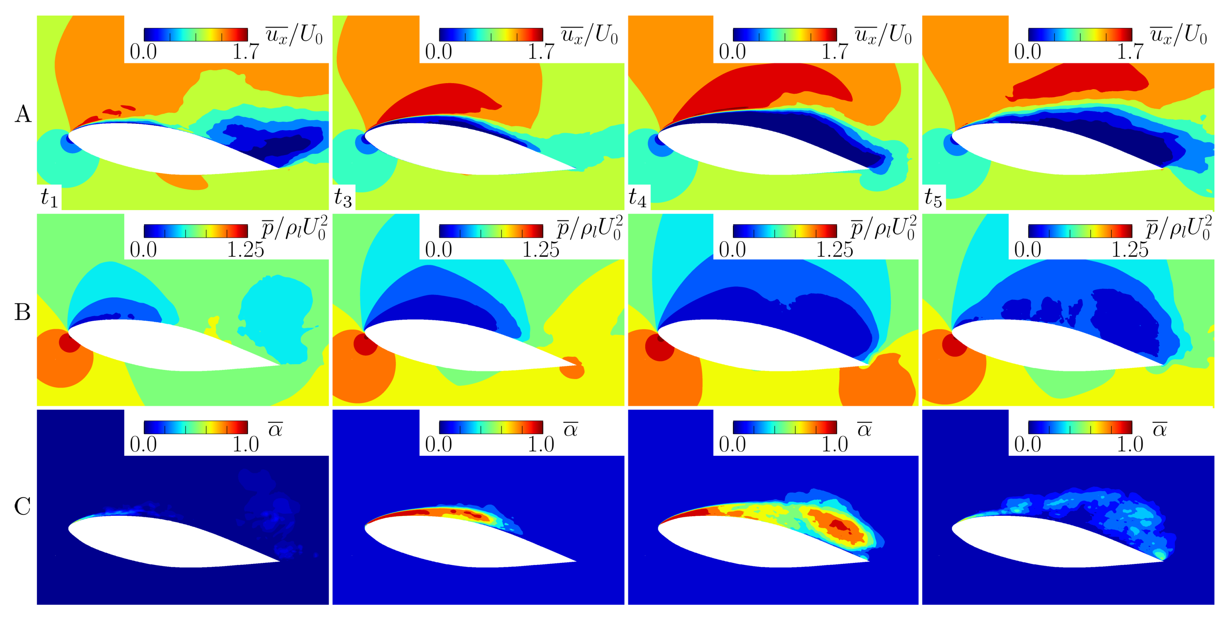
• The presence of cavitation structures was correlated with pressure fields and resultant forces, revealing a significant effect on flow dynamics.

This simulation method is a promising instrument for future numerical research to gain insight into the physics of unsteady sheet/cloud cavitation and to develop control methods for mitigating its negative effects.

References

1. Plesset, M. Bubble dynamics and cavitation. Annu. Rev. Fluid Mech. 1977, 9, 145–185. [Google Scholar] [CrossRef]
2. Arndt, R. Bubble dynamics and cavitation. Cavitation Fluid Mach. Hydraul. Struct. 1981, 13, 273–328. [Google Scholar]
3. Arndt, R. Cavitation in vortical flows. Annu. Rev. Fluid Mech. 2002, 34, 143–175. [Google Scholar]
4. Brennen, C. Cavitation and Bubble Dynamics; Cambridge University Press: Cambridge, UK, 2014. [Google Scholar]
5. Laberteaux, K.R.; Ceccio, S.L. Partial cavity flows. Part 1. Cavities forming on models without spanwise variation. J. Fluid Mech. 2001, 431, 1–41. [Google Scholar] [CrossRef]
6. Laberteaux, K.R.; Ceccio, S.L. Partial cavity flows. Part 2. Cavities forming on test objects with spanwise variation. J. Fluid Mech. 2001, 431, 43–63. [Google Scholar] [CrossRef]
7. Kjeldsen, M.; Arndt, R.E.A.; Effertz, M. Spectral characteristics of sheet/cloud cavitation. J. Fluids Eng. 2000, 112, 481–487. [Google Scholar] [CrossRef]
8. Callenaere, M.; Franc, J.P.; Michel, J.M.; Riondet, M. The cavitation instability induced by the development of a re-entrant jet. J. Fluid Mech. 2001, 444, 223–256. [Google Scholar] [CrossRef]
9. Pham, T.M.; Larrarte, F.; Fruman, D.H. Investigation of unsteady sheet cavitation and cloud cavitation mechanisms. J. Fluids Eng. 1999, 121, 289–296. [Google Scholar] [CrossRef]
10. Watanabe, S.; Tsujimoto, Y.; Furukawa, A. Theoretical analysis of transitional and partial cavity instabilities. J. Fluids Eng. 2001, 123, 692–697. [Google Scholar]
11. Timoshevskiy, M.V.; Churkin, S.A.; Kravtsova, A.Y.; Pervunin, K.S.; Markovich, D.M.; Hanjalić, K. Cavitating flow around a scaled-down model of guide vanes of a high-pressure turbine. Int. J. Multiph. Flow 2016, 78, 75–87. [Google Scholar] [CrossRef]
12. Kawanami, Y.; Kato, H.; Yamaguchi, H.; Tanimura, M.; Tagaya, Y. Mechanism and control of cloud cavitation. J. Fluids Eng. 1997, 119, 788–794. [Google Scholar] [CrossRef]
13. Kubota, A.; Kato, H.; Yamaguchi, H.; Maeda, M. Unsteady structure measurement of cloud cavitation on a foil section using conditional sampling technique. J. Fluids Eng. 1989, 111, 204–210. [Google Scholar] [CrossRef]
14. Ganesh, H.; Makiharju, S.A.; Ceccio, S.L. Bubbly shock propagation as a mechanism for sheet-to-cloud transition of partial cavities. J. Fluid Mech. 2016, 802, 37–78. [Google Scholar] [CrossRef]
15. Reisman, G.E.; Wang, Y.C.; Brennen, C.E. Observations of shock waves in cloud cavitation. J. Fluid Mech. 1998, 355, 255–283. [Google Scholar]
16. Leroux, J.B.; Astolfi, J.A.; Billard, J.Y. An experimental study of unsteady partial cavitation. J. Fluids Eng. 2004, 126, 94–101. [Google Scholar] [CrossRef]
17. Ji, B.; Luo, X.W.; Arndt, R.E.; Peng, X.; Wu, Y. Large eddy simulation and theoretical investigations of the transient cavitating vortical flow structure around a NACA66 hydrofoil. Int. J. Multiph. Flow 2015, 68, 121–134. [Google Scholar]
18. Zhang, G.; Wang, Z.; Wu, C.; Li, H.; Sun, T. Numerical investigation of multistage cavity shedding around a cavitating hydrofoil based on different turbulence models. Ocean Eng. 2023, 284, 115248. [Google Scholar] [CrossRef]
19. Bhatt, A.; Ganesh, H.; Ceccio, S.L. Partial cavity shedding on a hydrofoil resulting from re-entrant flow and bubbly shock waves. J. Fluid Mech. 2023, 957, A28. [Google Scholar] [CrossRef]
20. Kawakami, D.T.; Fuji, A.; Tsujimoto, Y.; Arndt, R.E.A. An assessment of the influence of environmental factors on cavitation instabilities. J. Fluids Eng. 2008, 130, 031303. [Google Scholar] [CrossRef]
21. Decaix, J.; Goncalves, E. Investigation of three-dimensional effects on a cavitating venturi flow. J. Heat Fluid Flow 2013, 44, 576–595. [Google Scholar] [CrossRef]
22. Prothin, S.; Billard, J.Y.; Djeridi, H. Image processing using POD and DMD for the study of cavitation development on a NACA0015. In Proceedings of the 13th Journées de l’Hydrodynamique, Laboratoire Saint-Venant, Chatou, France, 21–23 November 2012. [Google Scholar]
23. Watanabe, S.; Yamaoka, W.; Furukawa, A. Unsteady lift and drag characteristics of cavitating Clark Y-11.7% hydrofoil. IOP Conf. Ser. Earth Environ. Sci. 2014, 22, 052009. [Google Scholar] [CrossRef]
24. Tsuru, W.; Ehara, Y.; Kitamura, S.; Watanabe, S.; Tsuda, S. Mechanism of lift increase of cavitating Clark Y-11.7% hydrofoil. In Proceedings of the 10th International Symposium on Cavitation (CAV2018), Baltimore, MD, USA, 14–16 May 2018. [Google Scholar]
25. Keller, A.P. Cavitation Scale Effects Empirically Found Relations and the Correlation of Cavitation Number and Hydrodynamic Coefficients. Lecture 001. 2001. Available online: https://caltechconf.library.caltech.edu/92/ (accessed on 17 August 2023).
26. Liu, Y.; Li, X.; Wang, W.; Li, L.; Huo, Y. Numerical investigation on the evolution of forces and energy features in thermo-sensitive cavitating flow. Eur. J. Mech. B/Fluids 2020, 84, 233–249. [Google Scholar] [CrossRef]
27. Zhao, W.G.; Zhang, L.X.; Shao, X.M. Numerical simulation of cavitation flow under high pressure and temperature. J. Hydrodyn. Ser. B 2011, 23, 289–294. [Google Scholar] [CrossRef]
28. Hong, F.; Yuan, J.; Zhou, B. Application of a new cavitation model for computations of unsteady turbulent cavitating flows around a hydrofoil. J. Mech. Sci. Technol. 2017, 31, 249–260. [Google Scholar] [CrossRef]
29. Matsunari, H.; Watanabe, S.; Konishi, Y.; Suefuji, N.; Furukawa, A. Experimental/numerical study on cavitating flow around Clark Y 11.7% hydrofoil. In Proceedings of the Eighth International Symposium on Cavitation, Singapore, 13–16 August 2012; pp. 358–363. [Google Scholar]
30. Deng, L.F.; Long, Y.; Cheng, H.Y.; Ji, B. Some notes on numerical investigation of three cavitation models through a verification and validation procedure. J. Hydrodyn. 2023, 35, 185–190. [Google Scholar] [CrossRef]
31. Arabnejad, M.; Amini, A.; Farhat, M.; Bensow, R. Numerical and experimental investigation of shedding mechanisms from leading-edge cavitation. Int. J. Multiph. Flow 2019, 119, 123–143. [Google Scholar] [CrossRef]
32. Long, Y.; Long, X.; Ji, B.; Xing, T. Verification and validation of Large Eddy Simulation of attached cavitating flow around a Clark-Y hydrofoil. Int. J. Multiph. Flow 2019, 115, 93–107. [Google Scholar] [CrossRef]
33. Chen, T.; Huang, B.; Wang, G. Numerical study of cavitating flows in a wide range of water temperatures with special emphasis on two typical cavitation dynamics. Int. J. Heat Mass Transf. 2016, 101, 886–900. [Google Scholar] [CrossRef]
34. Hsiao, C.T.; Ma, J.; Chahine, G.L. Multiscale tow-phase flow modeling of sheet and cloud cavitation. Int. J. Multiph. Flow 2017, 90, 102–117. [Google Scholar] [CrossRef]
35. Chen, Y.; Li, J.; Gong, Z.; Chen, X.; Lu, C. Large eddy simulation and investigation on the laminar-turbulent transition and turbulence-cavitation interaction in the cavitating flow around hydrofoil. Int. J. Multiph. Flow 2019, 112, 300–322. [Google Scholar] [CrossRef]
36. Pendar, M.R.; Esmaeilifar, E.; Roohi, E. LES study of unsteady cavitation characteristics of a 3-D hydrofoil with wavy leading edge. Int. J. Multiph. Flow 2020, 132, 103415. [Google Scholar] [CrossRef]
37. Li, D.; Miao, B.; Li, Y.; Gong, R.; Wang, H. Numerical study of the hydrofoil cavitation flow with thermodynamic effects. Renew. Energy 2021, 169, 894–904. [Google Scholar] [CrossRef]
38. Liu, H.; Tang, F.; Yan, S.; Li, D. Experimental and numerical studies of cloud cavitation behavior around a reversible S-shaped hydrofoil. J. Mar. Sci. Eng. 2022, 10, 386. [Google Scholar] [CrossRef]
39. Sun, T.; Wang, Z.; Zou, L.; Wang, H. Numerical investigation of positive effects of ventilated cavitation around a NACA66 hydrofoil. Ocean Eng. 2020, 197, 106831. [Google Scholar] [CrossRef]
40. Yin, T.; Pavesi, G.; Pei, J.; Yuan, S. Numerical investigation of unsteady cavitation around a twisted hydrofoil. Int. J. Multiph. Flow 2021, 135, 103506. [Google Scholar] [CrossRef]
41. Ivashchenko, E.; Hrebtov, M.; Timoshevskiy, M.; Pervunin, K.; Mullyadzhanov, R. Systematic validation study of an unsteady cavitating flow over a hydrofoil using conditional averaging: LES and PIV. J. Mar. Sci. Eng. 2021, 9, 1193. [Google Scholar] [CrossRef]
42. Timoshevskiy, M.V.; Ilyushin, B.B.; Pervunin, K.S. Statistical structure of the velocity field in cavitating flow around a 2D hydrofoil. Int. J. Heat Fluid Flow 2020, 85, 108646. [Google Scholar] [CrossRef]
43. Sagaut, P.; Adams, N.; Garnier, E. Large-Eddy Simulation for Compressible Flows; Springer: Berlin/Heidelberg, Germany, 2009. [Google Scholar]
44. Yoshizawa, A.; Horiuti, K. A statistically-derived subgrid-scale kinetic energy model for the large-eddy simulation of turbulent flows. J. Phys. Soc. Jpn. 1985, 54, 2834–2839. [Google Scholar] [CrossRef]
45. Schnerr, G.; Sauer, J. Physical and numerical modeling of unsteady cavitation dynamics. In Proceedings of the Fourth International Conference on Multiphase Flow, New Orleans, LO, USA, 27 May–1 June 2001; ICMF New Orleans: New Orleans, LO, USA, 2001; Volume 1. [Google Scholar]
46. Project Site OpenFOAM. 2004. Available online: http://www.openfoam.com (accessed on 17 August 2023).
47. Warming, R.F.; Beam, R. Upwind second-order difference schemes and applications in aerodynamic flows. Aiaa J. 1976, 14, 1241–1249. [Google Scholar] [CrossRef]
48. Van Leer, B. Towards the ultimate conservative difference scheme. II. Monotonicity and conservation combined in a second-order scheme. J. Comput. Phys. 1974, 14, 361–370. [Google Scholar] [CrossRef]
49. Crank, J.; Nicolson, P. A practical method for numerical evaluation of solutions of partial differential equations of the heat-conduction type. In Mathematical Proceedings of the Cambridge Philosophical Society; Cambridge University Press: Cambridge, UK, 1947; Volume 43, pp. 50–64. [Google Scholar]
50. Moukalled, F.; Mangani, L.; Darwish, M. The Finite Volume Method in Computational Fluid Dynamics; Springer: Berlin/Heidelberg, Germany, 2016. [Google Scholar]
51. Jasak, H. Error Analysis and Estimation for the Finite Volume Method with Applications to Fluid Flows; Imperial College London, University of London: London, UK, 1996. [Google Scholar]
52. Ferziger, J.H.; Perić, M.; Street, R.L. Computational Methods for Fluid Dynamics; Springer: Berlin/Heidelberg, Germany, 2002. [Google Scholar]
53. OpenFOAM Dynamic Mesh Refine Library. 2019. Available online: http://voluntary.holzmann-cfd.de/software-development/libraries/direfinefvmesh (accessed on 17 August 2023).
54. Cadieux, F.; Sun, G.; Domaradzki, J.A. Effects of numerical dissipation on the interpretation of simulation results in computational fluid dynamics. Comput. Fluids 2017, 154, 256–272. [Google Scholar]
55. Kravtsova, A.Y.; Markovich, D.M.; Pervunin, K.S.; Timoshevskiy, M.V.; Hanjalic, K. High-speed visualization and PIV measurements of cavitating flows around a semi-circular leading-edge flat plate and NACA0015 hydrofoil. Int. J. Multiph. Flow 2014, 60, 119–134. [Google Scholar] [CrossRef]
56. Ilyushin, B.B.; Timoshevskiy, M.V.; Pervunin, K.S. Vapor concentration and bimodal distributions of turbulent fluctuations in cavitating flow around a hydrofoil. Int. J. Heat Fluid Flow 2023, 103, 109197. [Google Scholar] [CrossRef]
57. Roache, P.J. Verification and Validation in Computational Science and Engineering; Hermosa: Albuquerque, NM, USA, 1998; Volume 895, p. 895. [Google Scholar]
Figure 1. Computational domain: a rectangular channel along 4.3 C with scaled-down model of guide vanes of a Francis turbine at a moderate angle of attack of 9°; boundary conditions and the coordinate system. Blow-up demonstrates the process of dynamic mesh refinement by depicting an instantaneous vapor volume field α ˜ .
Energies 16 06990 g001
Figure 2. Instantaneous velocity vector fields around the hydrofoil from PIV (A) and LES (B) at the hydrofoil midspan. Dashed black-white vertical lines in the left image denote cross-sections for which profiles of various turbulence quantities are presented below (denoted 15).The red and gray isosurfaces in the right image indicate areas occupied by the vapor phase with α ˜ = 0.25 and 0.5 , respectively.
Energies 16 06990 g002
Figure 3. Comparison of PIV [11] and LES results for the streamwise component of the mean liquid velocity (A) and its streamwise fluctuations (squared values) (B) in the five cross-sections, marked in Figure 2, along the midspan section of the hydrofoil at x / C = 0.4 , 0.2 , 0.0 , 0.2 , and 0.4 (denoted 15). The numerical data are presented together in form of time-averaged ( . ) ¯ and conditionally averaged . α ˜ t h profiles according to Equation (9). The threshold value of α ˜ t h is chosen to be equal to 0.25 .
Energies 16 06990 g003
Figure 4. (A) Evolutionof C L and C D for a long time interval. (B) Blow-up of the same evolution curves for a shorter time interval. Dashed lines show the time-averaged values C ¯ D and C ¯ L . Red dots denote specific time instants corresponding to the local maximum, values between the extrema and zero, and minimum of C L . Simbol * denote time instant corresponding to start of the next cycle.
Energies 16 06990 g004
Figure 5. Instantaneous isosurfaces of α ˜ = 0.1–0.9 (A), velocity vector field near the hydrofoil surface (B) and nondimensional Q = 2.5 are colored with streamwise velocity u x (C) on the hydrofoil surface at several typical moments in one cloud cavitation shedding cycle (stages from t 1 to t 1 * ). Simbol * denote time instant corresponding to start of the next cycle.
Energies 16 06990 g005
Figure 6. Evolution of C L for a short time interval. Red dots denote specific time instants corresponding to the local maximum, values between the extrema and zero, and minimum of C L .
Energies 16 06990 g006
Figure 7. Conditional average fields of streamwise velocity (A), pressure (B), and α ˜ (C) for four specific time moments: minimum t 1 , average value before maximum t 3 , maximum t 4 , and average value after maximum of C L t 5 .
Energies 16 06990 g007
Figure 8. (A) Snapshots captured in the experiment (bottom row) and isosurface α ˜ = 0.1–0.9 from LES (top row). (B) Frequency spectrum of intensity level I z and the vapor volume fraction α z averaged over time and spanwise direction and normalized by the maximum value. (C) Short time history of the instantaneous vapor volume fraction α z averaged over spanwise direction and isosurfaces of α ˜ = 0.1–0.9 for the stages t 2 , t 3 , and t 5 . Simbol * denote time instant corresponding to start of the next cycle.
Energies 16 06990 g008