Research on Terrain Mobility of UGV with Hydrostatic Wheel Drive and Slip Control Systems

Abstract

The article explored the potential for enhancing the off-road mobility of unmanned ground vehicles (UGV) equipped with a hydrostatic drive system. The analysis showed that effectively overcoming rough or soft terrain demands a slip limitation. In the UGVs with hydrostatic drives, flow dividers are used for this purpose. Unfortunately, they have certain drawbacks, such as reduced efficiency due to pressure losses. In order to minimize this phenomenon, an external braking system was used as a new slip control system. Therefore, simulation studies were carried out to assess the new slip control system while overcoming terrain obstacles due to the reduction of energy consumption and improving the mobility of the UGV.

1. Introduction

High mobility unmanned ground vehicles (UGVs) should possess the capabilities of crossing terrain with a low soil bearing capacity or low traction coefficient, as well as overcoming terrain obstacles such as ditches, embankments, logs, walls, curbs, etc. Their typical operational speeds range from 1 to 5 km/h, with maximum speeds reaching 8–12 km/h [1,2,3,4,5,6,7,8,9,10,11,12,13,14,15,16,17,18,19,20,21,22,23,24,25,26,27,28,29,30,31,32,33,34,35,36]. The most commonly encountered gear systems in high mobility UGVs are rubber belt track systems or wheeled systems [1,4,5,7,8,9,10,11]. Track-based systems used in UGVs provide low ground pressures [12,13], however, their main drawback is significant resistance to motion caused by the high energy consumption of the rubber belt track bending and substantial turning resistance [11,14,15]. An alternative option is wheeled systems, which exhibit low rolling resistance and lower mass compared to track-based systems [7,11,12,16].

For high mobility UGVs weighing over 300 kg, hydrostatic drive systems are often employed, as they enable stepless speed control and provide resistance to over-loading and overheating [1,3,5,8,12,17,18,19,20,21,22]. They also offer great flexibility in arranging the drive system and allow for the utilization of low-speed/high-torque hydrostatic motors, which can be directly mounted on the wheels or sprockets.

The parallel connection of the pump with the motors directed to drive the wheels (Figure 1) ensures the achievement of an open differential effect. This enables easy differentiation of wheel speeds, with very low internal resistance [7,16,20,23]. The achieved high kinematic flexibility reduces turning resistance and limits tire wear when driving on hard surfaces. On the other hand, during off-road driving, the high kinematic flexibility of the driveline, restricts the ability to develop driving force on the wheels, due to changes in the coefficient of traction or the normal forces in the ground contact area [12,13,19,20,21].

Increasing the driving forces requires limiting wheel slip [12,13,23,24,25,26,27,28,29]. The reduction in slip can also improve the braking performance and stability of the movement of the vehicle [30,31,32,33,34]. In the case of hydrostatic systems, satisfactory results in the wheel slip limitation are achieved by implementing flow dividers and appropriate types of hydraulic motors [37,38]. Better results can be obtained by using suitable control systems [35,36,39,40]. Moreover, Belyaev demonstrated [41] that active wheel speed and slip control, achieved by varying the pump’s flow, provide higher power transmission efficiency compared to mechanical systems.

The presented research concerns high-speed vehicles moving on flat surfaces. The task of the control systems is to prevent excessive speed differentiation. In this case, the kinematic discrepancy and the need to vary the wheel speeds occur only when the vehicle is turning. This phenomenon can be relatively easily included in the control algorithms, taking into account the operation of the steering system. However, UGVs have to move in rough terrain at low speeds and, moreover, cannot utilize inertial forces to overcome obstacles as high-speed vehicles do. Continuous development of significant traction forces on all wheels is necessary for traversing obstacles and driving over rough terrain. This requires differentiating the speed of wheels to maintain optimal slip for each wheel. The challenge is high kinematic discrepancy [42,43,44,45] caused by random terrain irregularities and obstacles, for which standard slip control systems cannot compensate [41]. Enhancing terrain mobility and obstacle-overcoming capabilities of UGVs necessitates individual wheel slip control despite considerable speed variation among them.

Analyzing the possibilities of controlling the rotational speed of hydraulic motors, two groups of solutions emerge: systems utilizing an external braking system and systems with active flow throttling [30,31,35,39]. Systems based on external brake systems are commonly used in cars today, known as anti-slip regulation (ASR) and electronic slip reduction (ESR). They are standard equipment in most passenger cars and work well under road conditions (usually: no off-road obstacles, high driving speeds, good ground load capacity, and traction). Additionally, the driver controls the car from the inside, directly feeling the car’s behavior and being able to respond to it. In cars, they are primarily safety systems, not solutions for overcoming obstacles and ultimately off-road mobility. Unmanned ground vehicles (UGVs) mostly move at very low speeds, overcoming large terrain obstacles, often in conditions of limited traction and load capacity. Additionally, they are remotely controlled. Therefore, the use of ASR/ESR-like solutions for UGVs should be considered as one of the possibilities, that needs to be verified. For machines and vehicles equipped with hydrostatic drive systems, a similar effect of reducing the rotational speed of the wheels and consequently controlling their slip can be achieved through systems with active flow throttling. However, the introduction of throttling elements causes a drop in the efficiency of the drive system and significantly higher energy consumption, which is still the subject of many studies [46,47,48,49,50,51,52,53]. Therefore, this solution is not considered.

One of the challenges in modeling a slip control system is selecting the method of activation action. Currently, in automotive safety systems, regulators using fuzzy logic are commonly used and utilized [54,55,56,57,58]. A very promising way of modeling involves the use of artificial intelligence. This method allows for modeling complex phenomena using relatively simple mathematical functions [59,60,61,62]. They are characterized by quite high reliability, while the internal operation of the system can be described as a black box in which we do not have a certain influence on the method of operation, only on the output signal.

Another approach is modeling using conventional mathematical functions such as the logistic function: Sigmoidal equation, tanh, bounded exponential, exponential [63,64,65,66]. Such characteristics, despite certain limitations in shaping the course of functions, have quite important features such as the ability for analytical verification of the model or the possibility of parametric influence directly on the shape of the activation function. Among the above, tanh was chosen due to the ease of parametric shaping of the function’s course between two states.

The aim of the conducted research was to determine the influence of alternative strategies and settings of the slip control system on UGV mobility while overcoming terrain obstacles at low speeds and to assess the effectiveness of speed and slip control systems. Furthermore, the research provides information regarding the selection of system parameters to ensure high mobility while considering the impact of its operation on energy consumption while overcoming obstacles.

2. Method

In order to determine the effect of slip control on the off-road mobility of the UGV, simulation studies were carried out. For this purpose, an advanced simulation model was built. It integrates both the hydraulic drive system and the mechanical structure of the vehicle, allowing for accurate mapping of the actual behavior of the vehicle in various conditions. The aim of the research was to evaluate the effectiveness of various settings of the slip control system when overcoming obstacles with different grips. The following values were used as efficiency indicators:

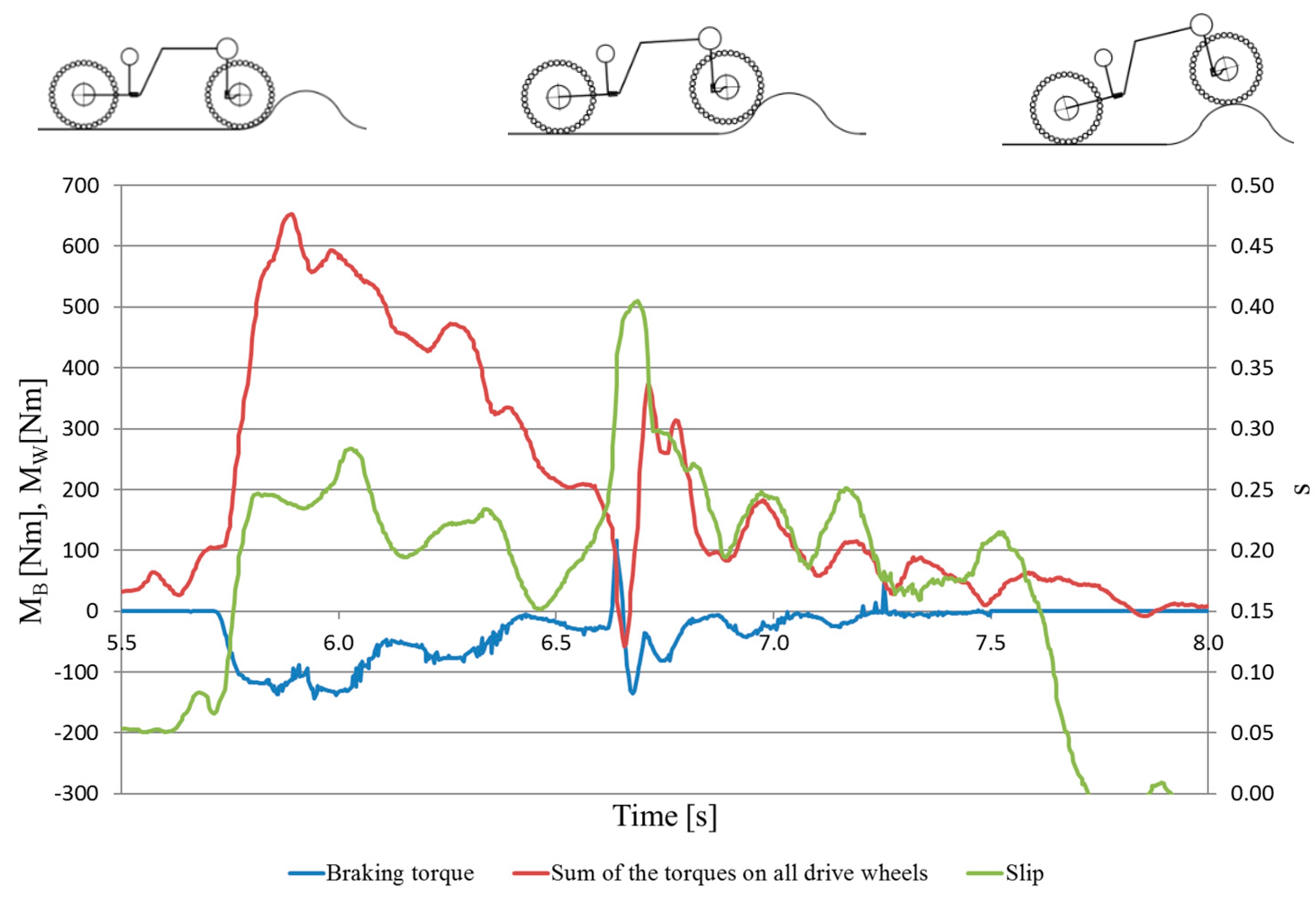
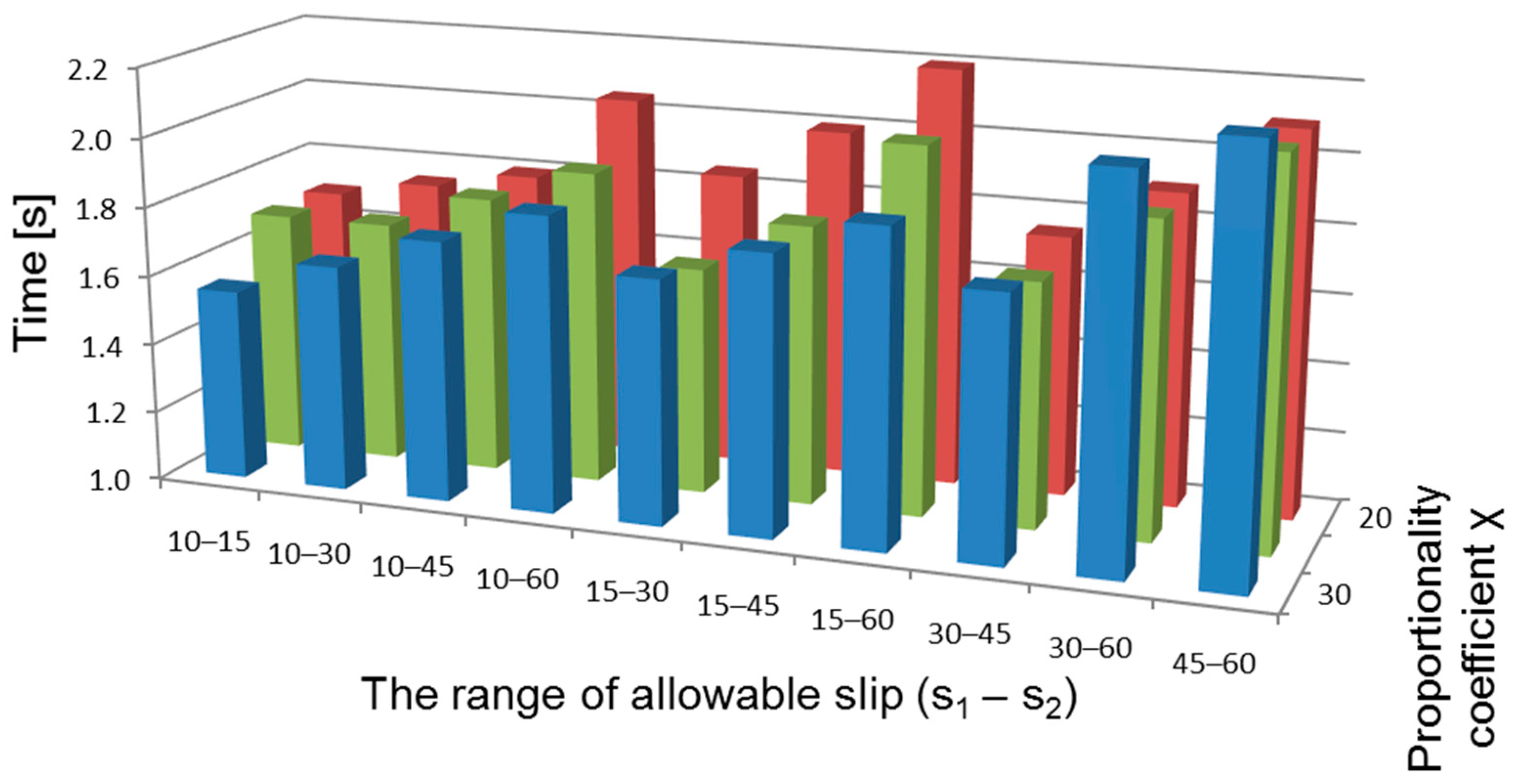
• − Time necessary to overcome the obstacle, t_d;
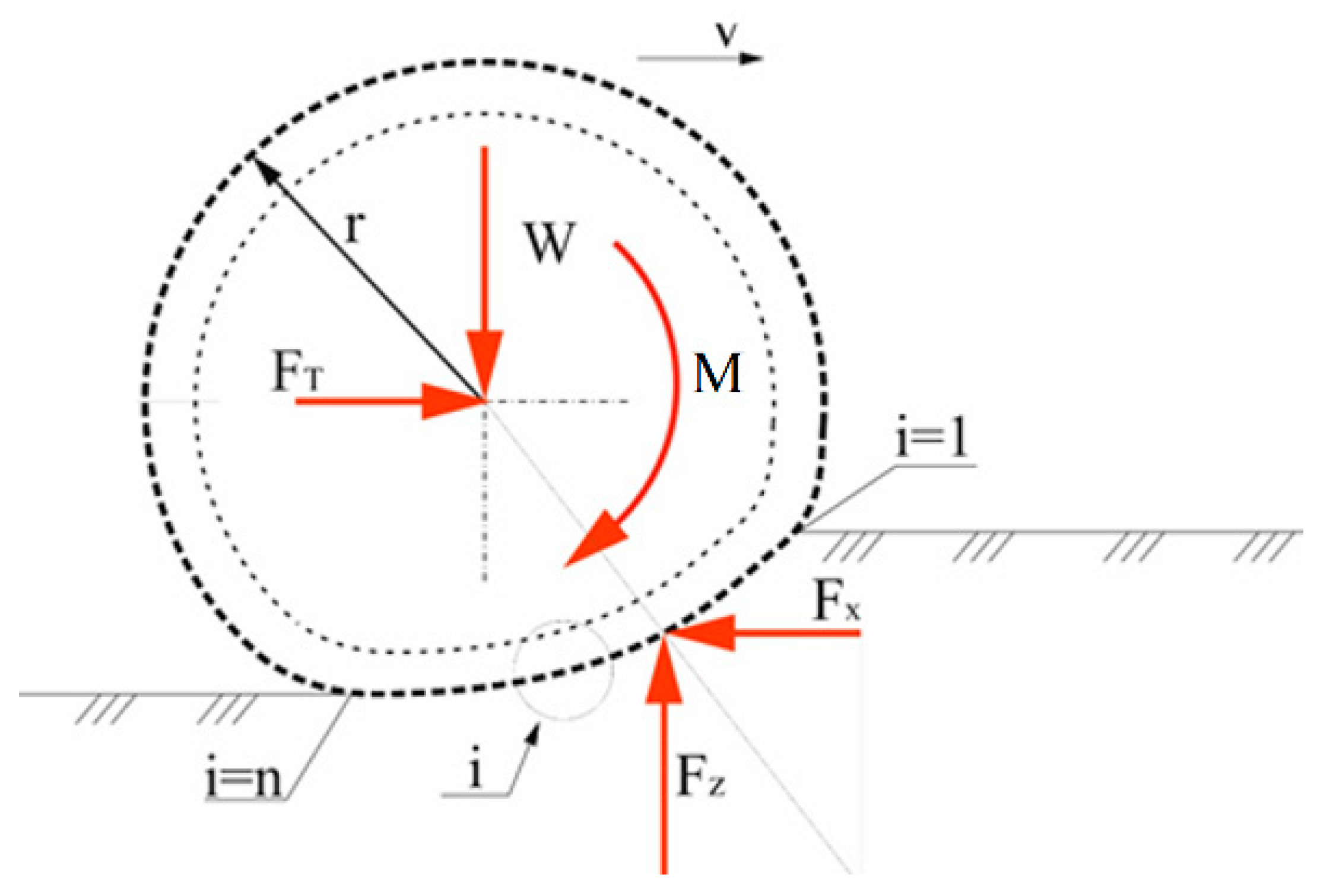
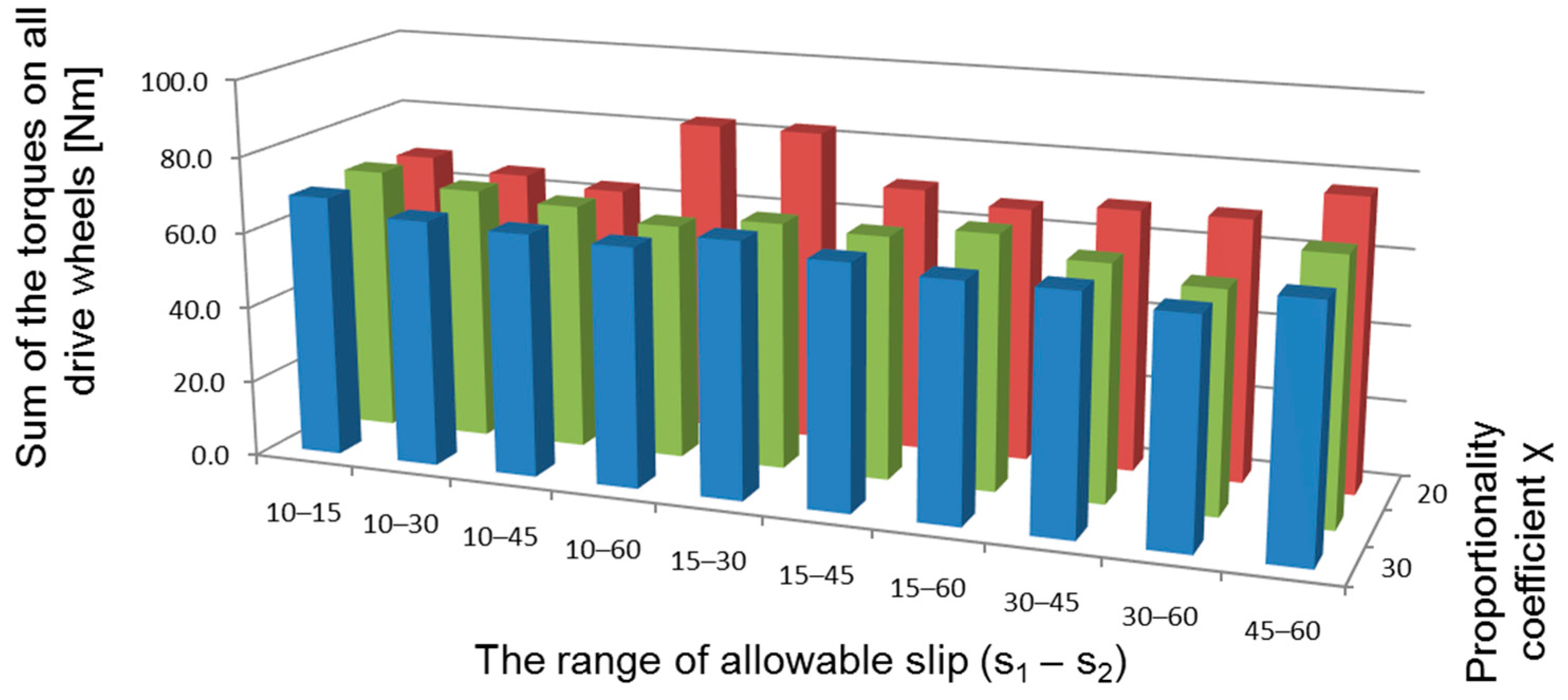
• − Maximum necessary drive torque on wheels M_W;
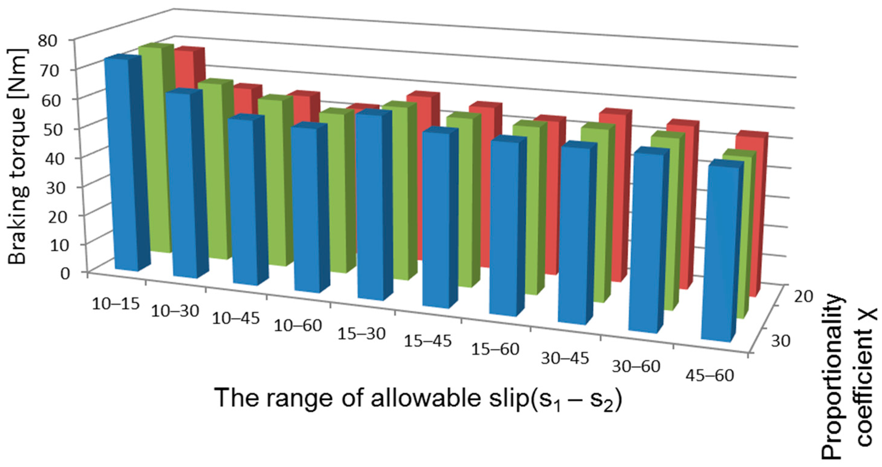
• − Maximum braking torque M_B;
• − Energy on wheels necessary to overcome an obstacle E_W.

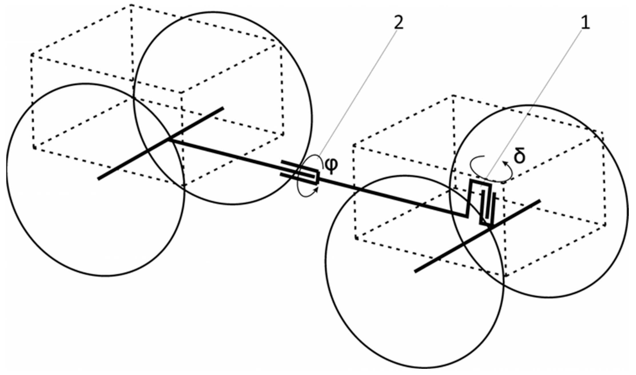
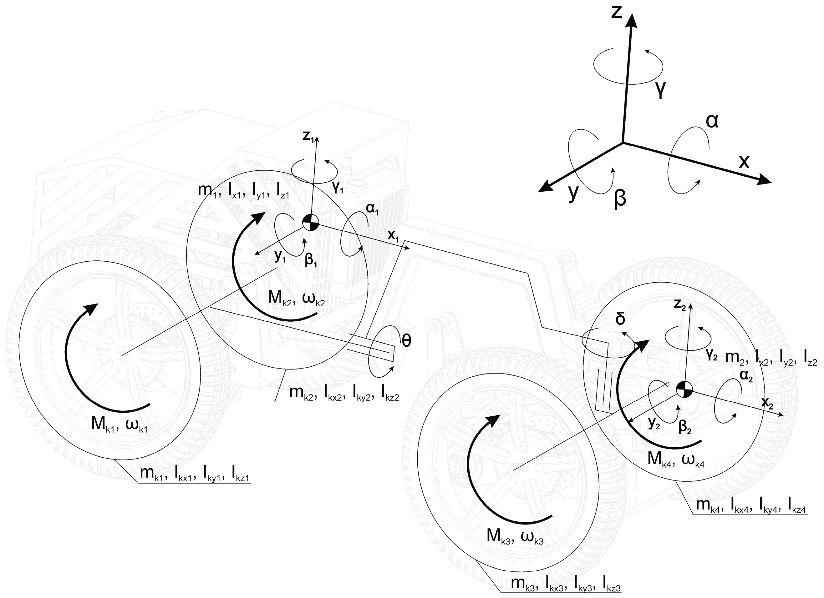
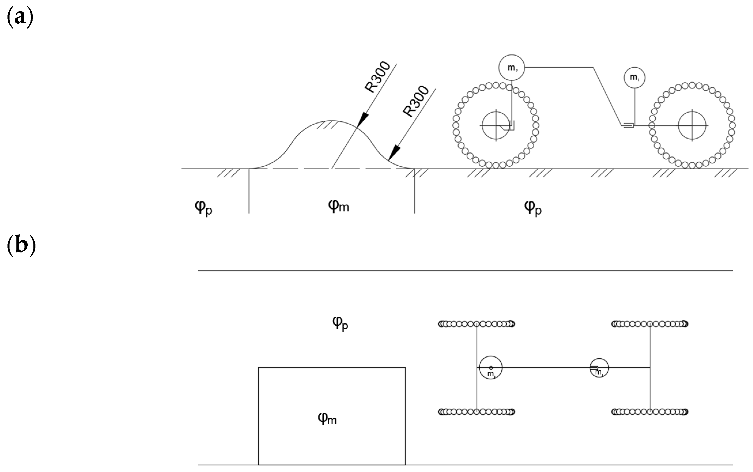
2.1. Light UGV Mechanical Structure Model

For the research, a simulation model of a lightweight, 300 kg, high mobility 4 × 4 articulated wheeled UGV with a wheel track of 0.90 m, wheelbase of 1.20 m, and wheel diameter of 0.60 m was used. It was assumed that the steering joint (1) is located above the front axle, and terrain copying would be ensured by an oscillating pin (2) (Figure 2).

In order to achieve smooth acceleration and stable driving at inching speeds, a hydrostatic drive system with one pump and four motors was used, as shown in Figure 3. The main parameters of the 4 × 4 high mobility UGV drive system are presented in

Table 1. Hydrostatic drivetrain parameters of light high mobility UGV model.

Parameter	Value
Engine max. power	N = 9.9 kW
Nominal engine speed	n = 3600 rpm
Pump max. displacement	qp = 18 cm3/rev
Hydraulic motor displacement	qs = 5 cm3/rev
Max. pump and motor pressure	31.5 MPa
Total final drive ratio	i = 19.3

.

A light high mobility UGV mechanical structure model (Figure 4) was developed with a multi-body method in Adams 2014.0.1 (MSC Software Corporation). The developed model consists of four wheels driven by hydrostatic motors with final drive according to Figure 3. The light high mobility UGV model has 7 DoF (angles displacement: α₁, β₁, γ₁, θ₁ translation displacement: x₁, y₁, z₁), considering the vehicle frame. The DOF does not take into account the wheel model due to its internal structural complexity. It was assumed that the steering angle of the frame is δ = 0. The holonomic constraints that were used in the vehicle model to connect its parts were ideal (without friction). Main values of light UGV model parameters are presented in

Table 2. Vehicle model main parameters (according to Figure 3).

Type	Parameter Value
Front body mass	m1 = 132 kg
Mass front body moment of inertia	I1x = 4.6 kg m2 I1y = 18.9 kg m2 I1z = 19.3 kg m2
Rear body mass	m2 = 127 kg
Mass rear body moment of inertia	I2x = 3.8 kg m2 I2y = 6.8 kg m2 I2z = 8.5 kg m2
Wheels mass	mk1 = mk2 = mk3 = mk4 = 5.36 kg
Mass wheel moment of inertia	Ikx1 = Ikx2 = Ikx3 = Ikx4 = 0.132 kg m2 Iky1 = Iky2 = Iky3 = Iky4 = 0.252 kg m2 Ikz1 = Ikz2 = Ikz3 = Ikz4 = 0.132 kg m2
Wheel radius	r = 0.30 m

.

The vehicle model uses a discrete model of a flexible wheel consisting of rigid bodies forming two rings: the tire carcass and tire tread. The discrete elements are connected to each other and to the rim by forces and torques derived from stiffness and damping in the radial and circumferential directions—Figure 5.

Each ring consists of 144 elements. Thus, it meets the computational efficiency requirements in accordance with the recommendations contained in [25]. The force positions acting on the wheels, which were taken into account in the developed wheel model, are shown in Figure 6.

Each element of the wheel tread in contact with the ground generates a traction force depending on the slip, the traction coefficient, and the normal reaction to the ground. The main wheel model parameters are presented in

Table 3. Main wheel model parameters.

Wheel Element	Parameter Type	Symbol	Parameter Value
Rim	Mass	mo	2.5 kg
	Inertia	Jo	0.520 kg m2
Carcass	Mass	m1	0.02 kg
	Inertia	J1	0.006 kg m2
	Number of elements	-	72
	Stiffness	kw1 kw2 kw3 kw4 kw5 kw6	100,000 N/m 100,000 N/m 1 Nm/rad 10,000,000 N/m 20 N/m 1 Nm/rad
	Damping	cw1 cw2 cw3 cw4 cw5 cw6	10,000 Ns/m 500 Ns/m 500 Nms/rad 100 Ns/m 100 Ns/m 1 Nms/rad
Tread	Mass	m2	0.02 kg
	Inertia	J2	0.006 kg m2
	Number of elements	-	72
	Stiffness	kw7 kw8 kw9 kw10 kw11 kw12	500,000 N/m 500,000 N/m 1 Nm/rad 5,000,000 N/m 5,000,000 N/m 1 Nm/rad
	Damping	cw7 cw8 cw9 cw10 cw11 cw12	500 Ns/m 500 Ns/m 0.1 Nms/rad 100 Ns/m 100 Ns/m 0.1 Nms/rad

.

The vertical load on the wheel is balanced by the sum of the vertical elementary forces—normal and circumferential—acting at the contact point of the tire with the ground (Figure 6), which, in the developed model, was determined based on the dependence:

$$W=F_z={{\displaystyle \sum }}_{i=1}^n\left(d{R}_{N,i}\cos \psi +d{R}_{T,i}\sin \psi \right)$$

(1)

where dR_N,i is the elementary normal reaction of the ground; dR_T,i is the elementary circumferential reaction of the ground. The traction force results from the sum in the horizontal components of normal and circumferential forces acting in contact with the ground (Figure 5), according to:

$$F_T=F_X={{\displaystyle \sum }}_{i=1}^n\left(d{R}_{T,i}\cos \psi +d{R}_{N,i}\sin \psi \right)$$

(2)

The developed model allowed us to obtain different traction coefficient φ depending on slip according to:

$$\phi \left(s\right)=\frac{F_T\left(s\right)}{F_z\left(s\right)}$$

(3)

Because slip is defined as ratio between theoretical wheel velocity (resulting from it angular velocity and dynamic radius) to actual velocity, this gives us the dependence of traction coefficient on the slip of the wheel model.

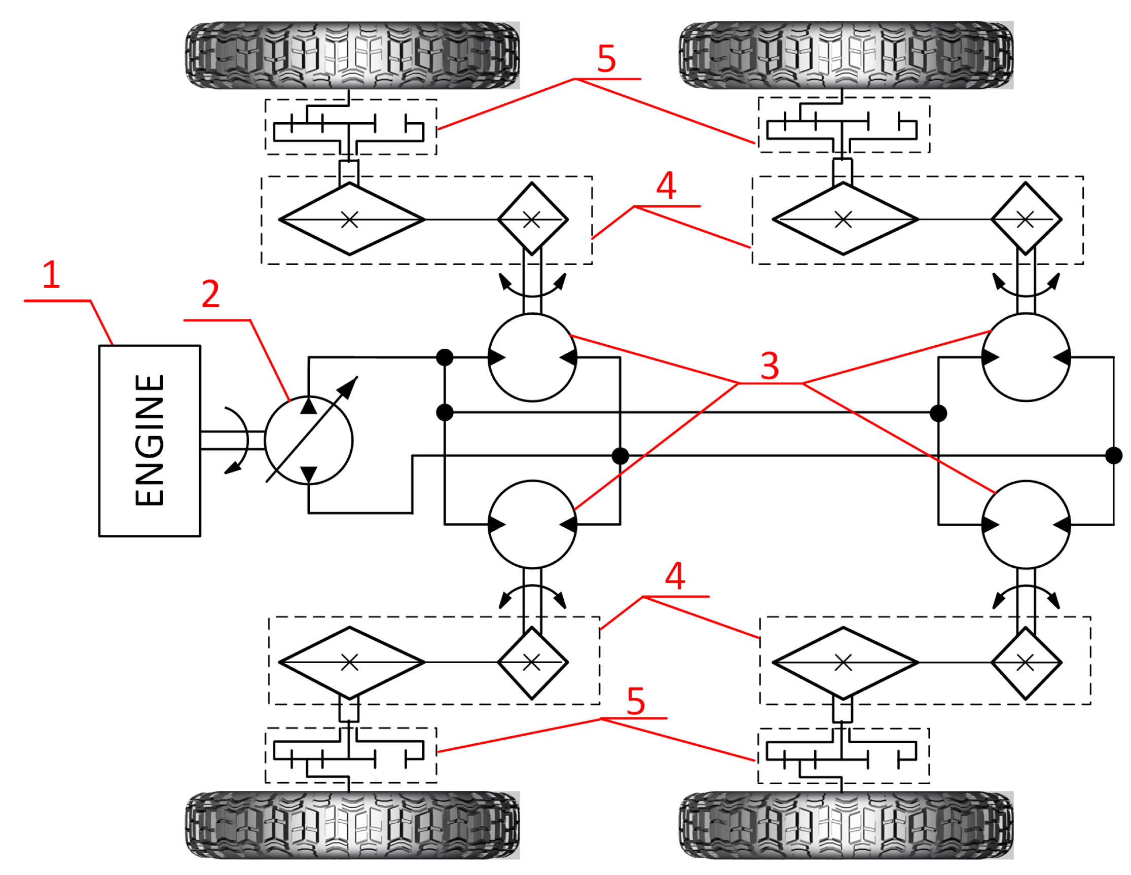
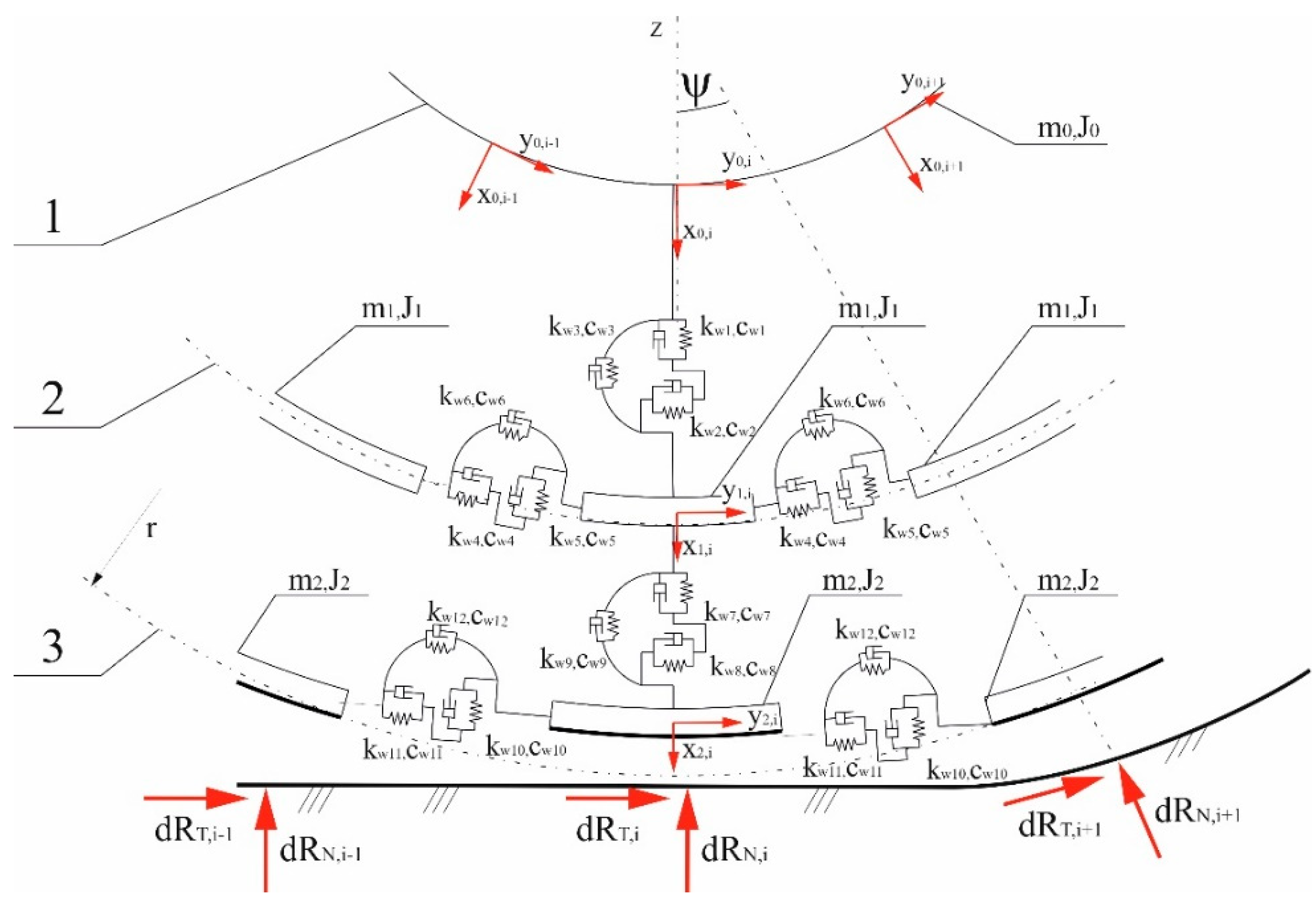
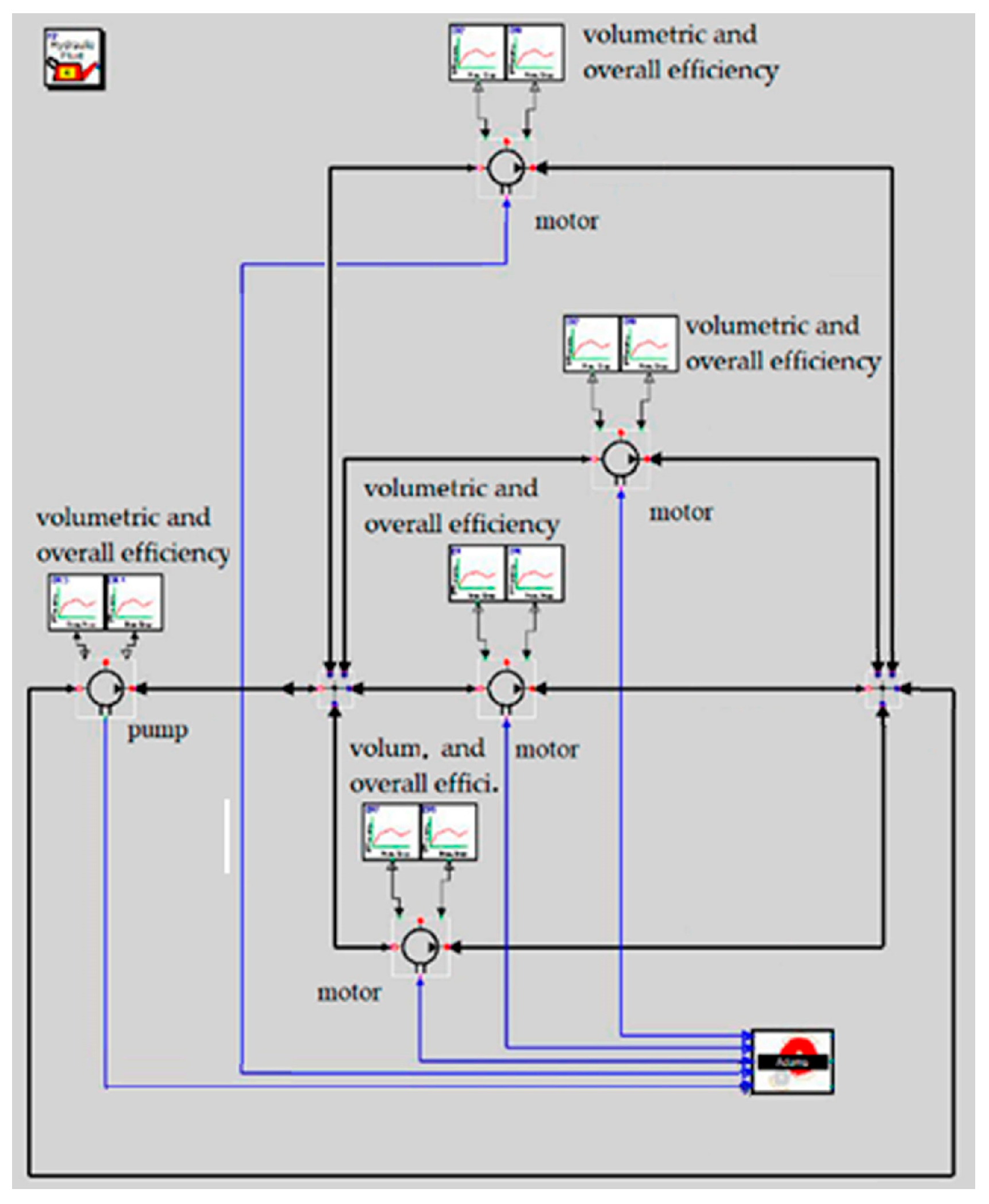
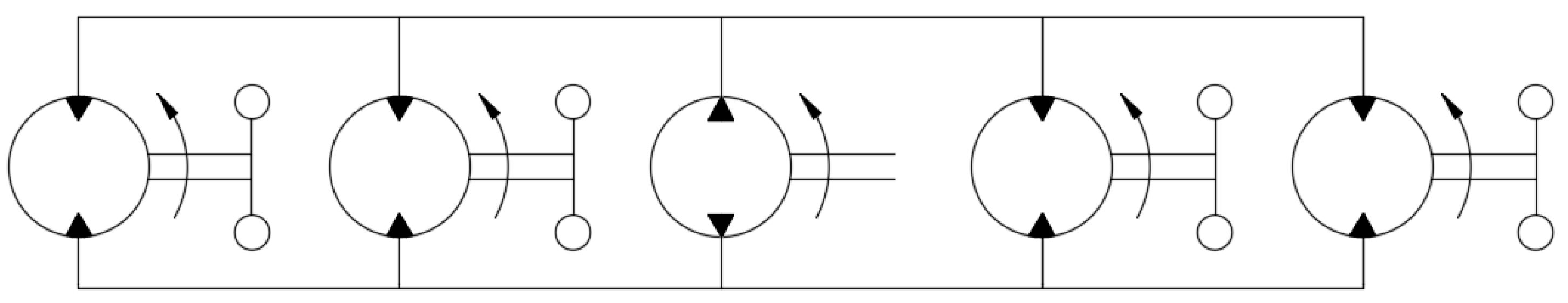
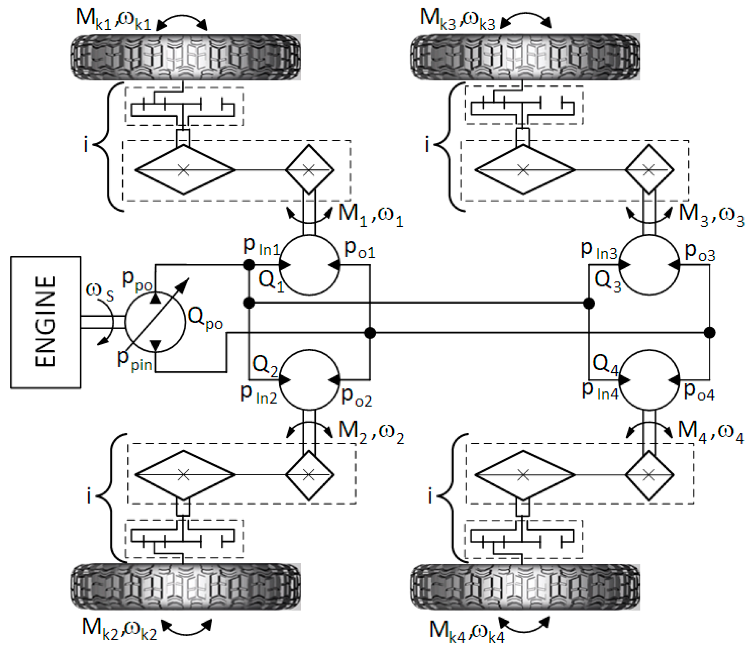
2.2. Light UGV Hydraulic Drivetrain Model

The hydraulic drivetrain model (Figure 7) for the light UGV model was developed in separate software (Easy5 2015.0.1 Version 9.1.1 (MSC Software Corporation)). The values that connect the vehicle body model and the hydraulic drivetrain model are as follows: drive torques on the wheels M_ki and their angular velocities ω_ki.

The generated driving torque M_ki by the i-th wheel, is transferred to corresponding hydraulic motor shaft through mechanical transmission (planetary and chain) with total final drive ratio i, and it can be calculated according to equation:

$$M_i=\frac{M_{ki}}{i}$$

(4)

where M_i—torque generated by the i–th hydraulic motor.

M_i torque caused increases in the pressure drop Dp_i on the hydraulic motor of this wheel:

$$\Delta p_i=p_{Ini}-p_{oi}$$

(5)

where p_Ini is the pressure on the input of the hydraulic motor; p_oi is the pressure on the output of hydraulic motor.

The pressure on hydraulic motor input depends on the pressure drop Dp_i and on the motor torque value M_i:

$$p_{Ini}=\frac{M_i}{q_s·\frac{{\eta }_{os}}{{\eta }_{vs}}}+p_{oi}$$

(6)

where q_s is the hydraulic motor displacement; h_os is the overall efficiency of the hydraulic motor; h_vs is the volumetric efficiency of the hydraulic motor. The overall and volumetric efficiency of hydraulic motors depends on the motor type and value of pressure and angular velocity, h_os, h_vs = f(Dp_i, w_i), which change during vehicle driving.

The pump output pressure p_po is greater than the value p_Ini shown by the pressure drop value Dp_i resulting from flow resistance occurring on the pipes/hoses Dp_Li and hydraulic connections Dp_mi, which are between the pump and the motor:

$$\Delta p_i=\Delta p_{Li}+\Delta p_{mi}$$

(7)

The pressure drop in the hydraulic pipes Dp_Li mainly depends on the value of the friction factor f, length i– th pipe/hose L_i, its internal diameter D_hLi, and flow velocity V_Li:

$$\Delta p_i=f\frac{L_i}{D_{hLi}}\frac{V_{Li}^2\rho }{2}$$

(8)

where r is the hydraulic oil density.

The flow velocity in the pipe/hose V_i depends on the value of the flow Q_i and internal pipe diameter D_hLi:

$$V_{Li}=\frac{4Q_i}{\pi D_{hLi}^2}$$

(9)

The value of the friction factor f depends on the of the flow character, classified on the basis of the Reynolds number:

$$R{e}_{Li}=\frac{\rho V_{Li}{D}_{hLi}}{\mu }$$

(10)

where m is the hydraulic oil dynamic viscosity.

For the laminar flow (Re_Li < 2000), the friction factor is calculated according to:

$$f=\frac{64}{R{e}_{Li}}$$

(11)

In the case of transition state (2000 ≤ Re_Li < 4000), the friction factor is calculated according to:

$$f=\frac{f_{4K}-f_{2K}}{2000}R{e}_{Li}+2f_{2K}-f_{4K}$$

(12)

where f_2K is the value of the friction factor calculated according to (11) for a Reynolds number value of 2000; f_4K is the value of the friction factor calculated according to (13) for a Reynolds number value of 4000.

For turbulent flow (4000 ≤ Re_Li ≤ Re_Lid), the friction factor is calculated according to:

$$\frac{1}{\sqrt{f}}=-2{\log }_{10}\left(\frac{\delta }{3.7}+\frac{2.51}{R{e}_{Li}\sqrt{f}}\right)$$

(13)

where d is the relative roughness, whereby:

$$R{e}_{Li\delta }=\frac{5000}{\delta }$$

(14)

For turbulent flow (Re_Li > Re_Lid), the friction factor has a constant value that depends only on the value of Re_Lid calculated according to (13) for Re_Li = Re_Lid.

The pressure drop occurs at the connection elements of hydraulic lines Dp_mi, which also depends on the flow character. For the laminar flow is calculated according to:

$$\Delta p_{mi}=\frac{Q_i·2\mu ·R{e}_T}{\pi ·D_h^3·C_d^2}$$

(15)

where D_h is the internal diameter of the connection element; C_d is the discharge coefficient Re_T is Reynolds number for turbulent flow.

For turbulent flow, the pressure drop is calculated according to:

$$\Delta p_{mi}=\frac{8\rho Q_i}{C_d^2·{\pi }^2·D_h^4}$$

(16)

Usually, to calculate the pressure drop for the connection elements, it is assumed that the transition to turbulent flow occurs at a Reynolds number of 100 (Re_T = 100). Therefore, there is almost always turbulent flow.

The pressure drop Dp_p on the pump is as follows:

$$\mathsf{\Delta }{p}_p=p_{po}-p_{pin}$$

(17)

where p_pin is the pump input pressure, which is usually 2 MPa for closed-circuit systems.

The flow Q_po generated by the pump depends mainly on its displacement q_p and the angular velocity of the shaft of the engine/pump w_p:

$$Q_{po}=\frac{60q_p{\omega }_p}{2\pi }{\eta }_{vp}$$

(18)

where h_vp is the volumetric efficiency of the pump; h_vp = f(Dp_p, w_p).

The angular velocity i-th hydraulic motor shaft w_i depends on the hydraulic motor displacement q_s and the flow Q_i:

$${\omega }_i=\frac{2\pi Q_i}{60q_s}{\eta }_{vs}$$

(19)

The angular velocity of i-th vehicle wheel w_i depends also on final drive ratio i according to relation:

$${\omega }_{ki}=\frac{{\omega }_i}{i}$$

(20)

The model of the hydrostatic drive system was implemented in the simulation environment Easy5 2015.0.1 Version 9.1.1 (MSC Software Corporation) Figure 8.

In the pump and motor models, the characteristics of the volumetric and overall efficiency were implemented, which were identified during the previously conducted laboratory tests [67] and are shown in Figure 9a–d.

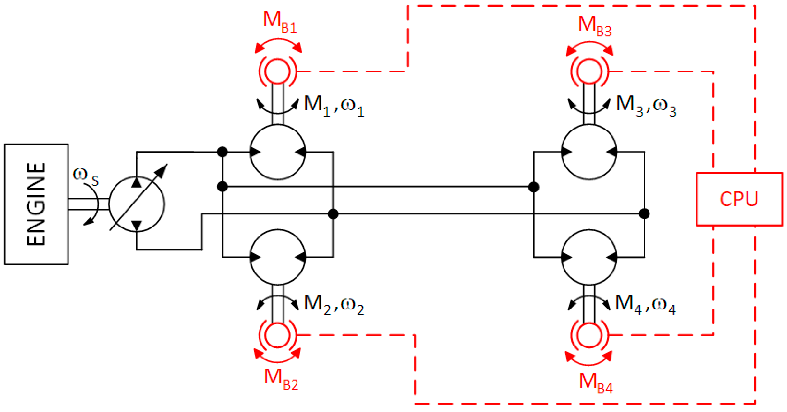
2.3. Slip Control System Model

In accordance with the research objective, the developed UGV model (Sections 2.1 and 2.2) enables slip control for each wheel. Since the hydraulic motors in the light UGV drive system are connected in parallel, if, for example, one of the wheels loses traction, it limits the pressure in the other motors and the ability to generate driving force on the other wheels. At the same time, the flow rate generated by the pump goes to the least loaded motor. This increases its rotational speed and wheel slip. As a result of the decrease in the driving force developed by all wheels, the UGV may stop. The slip control system should prevent this from happening.

In the tests, it was assumed that the system can brake individual wheels of the light UGV (generating the appropriate braking torque—M_Bi), increasing the motor load and its driving torque—M_ki. Increasing the external load on a particular hydraulic motor reduces the motor’s flow capacity and equalizes the flows in the motors. This is schematically illustrated in Figure 10.

The idea of the slip control system operation involves generating a signal to the wheel braking unit (M_Bi) by the CPU management unit, taking into account the current value of slip. For this purpose, the theoretical axle speed without slip (v_tki) was calculated by measuring the speed of each wheel (ω_ki):

v_tki=r_d · ω_ki

(21)

where: r_d—dynamic radius of the wheel.

Additionally, it was necessary to determine the actual forward speed of axle, for each wheel (v_rki). Based on this, the slip value of each wheel (s_i) was calculated:

$$s_i=\left(1-\frac{v_{rki}}{v_{tki}}\right)·100\%$$

(22)

In the model, a nonlinear (Figure 11) characteristic was assumed for the increase in the braking torque value M_Bi as a function of the wheel slip s_i. The activation of the slip control system (appearance of the braking torque) was determined by the initial slip s₁, and the slip s₂ causing the maximum braking torque M_Bmax.

To avoid sudden changes between the states of the braking torque values M_B0 and M_Bmax in the slip interval s₁–s₂, a function similar to the hyperbolic tangent was used. In the planned experiment, it was assumed that the parameters describing the shape of the characteristics influencing its course would be changed, as a result of which a family of 30 different characteristics implemented into the system was obtained.

The characteristic presented in Figure 11 can be described by the function:

$$M_B=\left\{\begin{array}{c}0 for s\le s_1\\ \alpha ·{\Delta }^2\left(3-2\Delta \right) for s_1<s<s_2\\ M_{Bmax} for s\ge s_2\end{array}\right.$$

(23)

The torque range coefficient α was determined from the following relation:

α = M_Bmax − M_B0

(24)

where:

∆ = (s − s₁)(s₂ − s₁)

(25)

s—current slip, s₁—activation point of the system, s₂—point of achieving the maximum value of the braking torque, M_Bmax—maximum value of the braking torque, M_B0—minimum value of the braking torque.

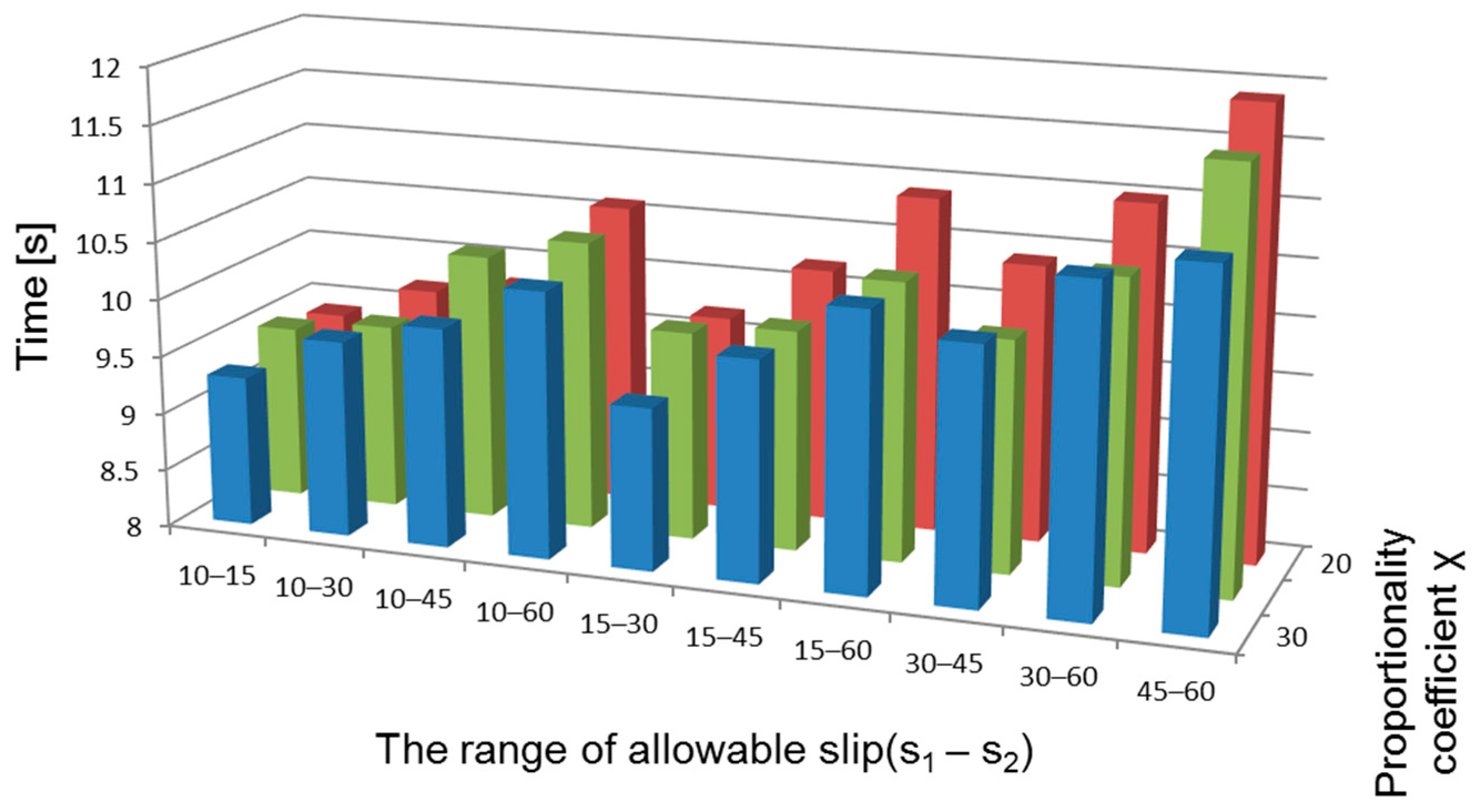
2.4. Analyzed Case Mobility of Light UGV

The research on the effectiveness of slip control systems for UGVs overcoming terrain obstacles at low speed was conducted considering two types of terrain obstacles:

a)

A ramp with slope of 15⁰ (Figure 12);

b)

A ground hummock (Figure 13).

In both cases (a) and (b), there were areas on the surface with different values of the maximum coefficient of traction. For inclines with a slope of 15°, these were zones with ϕ_p = 0.8, ϕ₁ = 0.05, ϕ₂ = 0.10, ϕ₃ = 0.15, and ϕ₄ = 0.20 (Figure 12) and for ground hummock obstacles, these were zones with ϕ_p = 0.8 and ϕ_m = 0.20 (Figure 13).

In the research, the braking characteristic (Figure 11) of the wheels was shaped by changing the parameters:

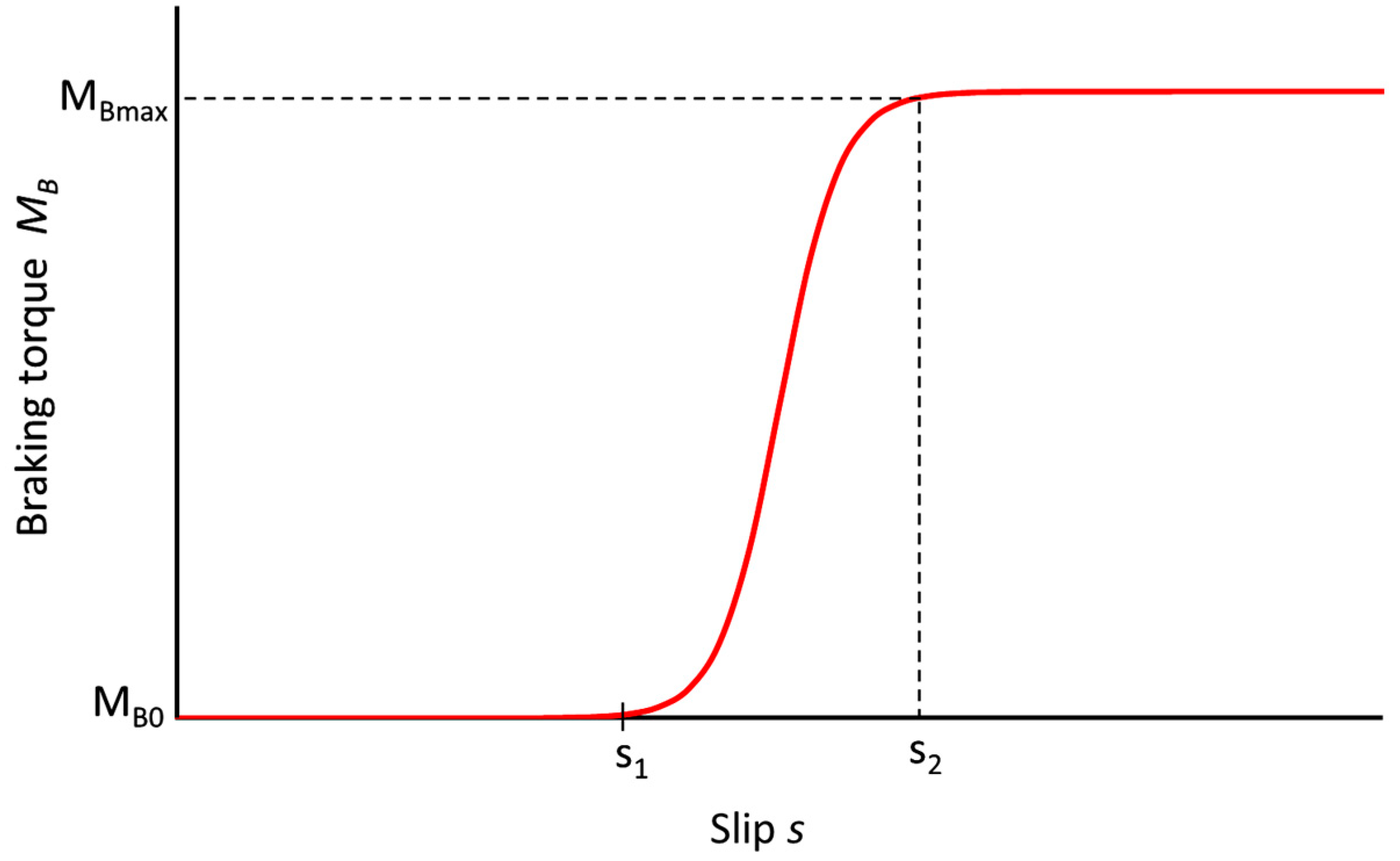
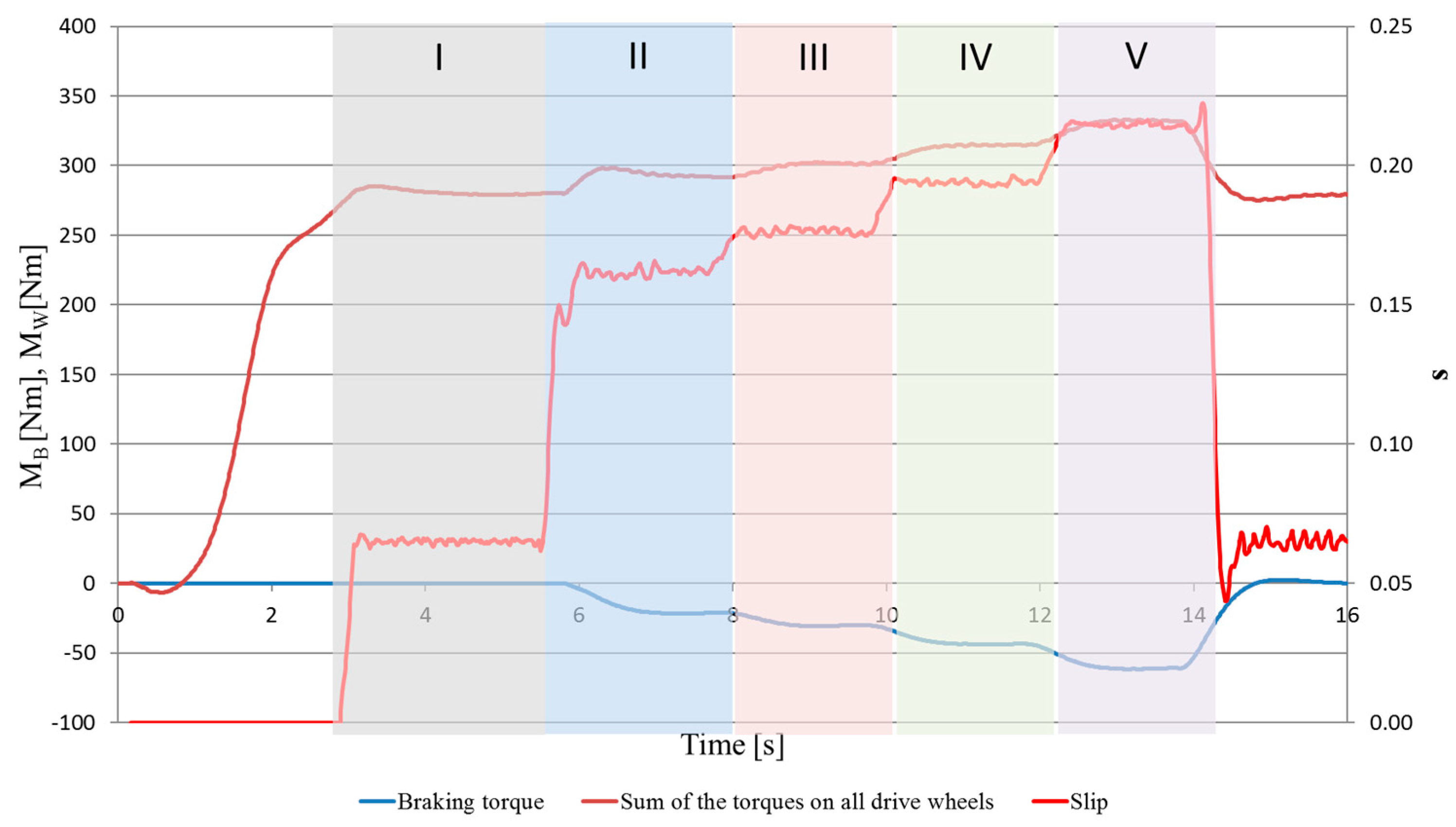
• Maximum braking torque M_Bmax in the i-th wheel;
• s₁—the slip control system is activated;
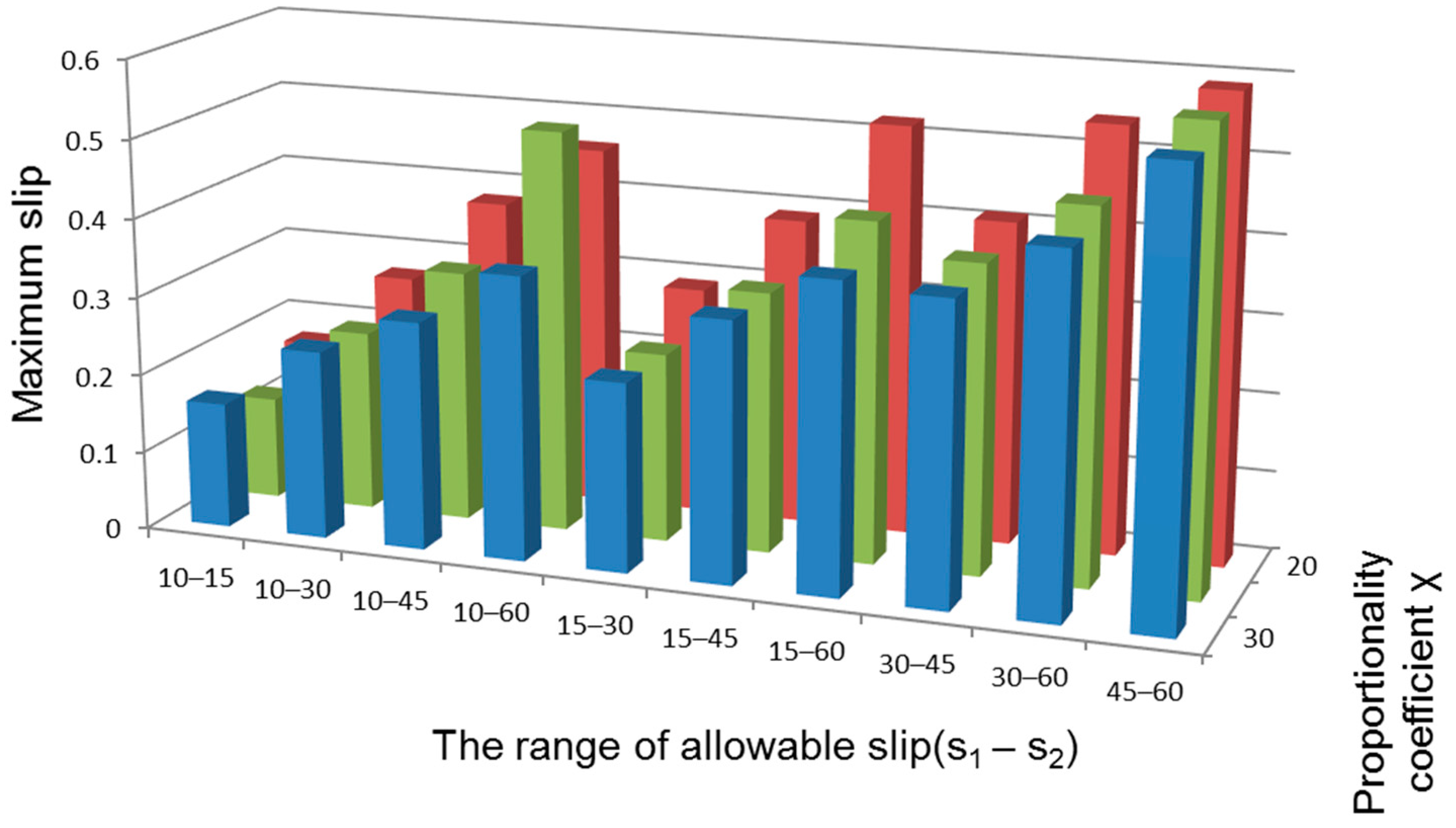
• s₂—the braking torque M_Bi reaches the maximum value M_Bmax.

The maximum value of the braking torque M_Bmax was determined proportionally to the sum of the moments M_w occurring on all drive wheels, according to the equation:

M_Bmax = cM_W

(26)

where: c—proportionality coefficient

M_w = M_k1 + M_k2 + M_k3 + M_k4

(27)

During research the coefficient χ was varied in the range of 5–30%, initial slip s₁ took values 0.10, 0.15, 0.30, and 0.45, and s₂ took values 0.15, 0.30, 0.45, and 0.6.

Energy on the wheels was calculated according to:

$$E_w=\underset{0}{\overset{t_d}{{\displaystyle \int }}}\left(F_T\left(t\right) v_{ki}\right) dt$$

(28)

where:

$$F_T\left(t\right)=\frac{M_{k1}\left(t\right)+M_{k2}\left(t\right)+M_{k3}\left(t\right)+M_{k4}\left(t\right) }{r_d}$$

(29)

In the ground model, zones with different maximum adhesion coefficient values were distinguished. In the ramp with slope model, local coefficients were ϕ₁ = 0.05, ϕ₁ = 0.10, ϕ₃ = 0.15, ϕ₄ = 0.20 oraz, ϕ_p = 0.80 for the rest of the ground. In the case of the ground hummock obstacle, the locally occurring maximum adhesion coefficient was ϕ_p = 0.80, ϕ_m = 0.20. Adhesion values are achieved at the assumed wheel slip values according to the function presented in (Figure 14). Results are similar to characteristics found in the paper [15].

In the conducted research, the pump flow was constant, corresponding to a UGV travel speed of 1 km/h on the section before the obstacle. The variations in speed during obstacle overcoming were caused by changes in resistance and slip. The studies revealed significant differences in the ability to overcome the specified obstacles depending on the parameter control settings (M_Bmax, s₁, s₂). For ramps, the slip was mainly caused by a decrease in the coefficient of traction, whereas in the case of ground hummock obstacles, it was affected by changes in the coefficient of traction and the distribution of wheels’ normal forces.

In the case of the platform model approaching a ramp, the time t_d was defined as the time interval starting from the moment the front left wheel of the platform model entered the zone with a coefficient of traction of ϕ₄ = 0.2, until the same wheel left the last zone with a coefficient of traction of ϕ₁ = 0.05. For the ground hummock obstacle, the time t_d was defined as the time interval starting from the moment the front left wheel made contact with the ground with a coefficient of traction of ϕ_m = 0.2, until the wheel reached the highest position at the top of the ground hummock.

3. Results

In the case of driving the UGV on a ramp, with braking torque (M_B) up to 0.15 M_w, the UGV was unable to climb the slop, or it took drastically more time compared to higher M_B values. At higher values of the braking torque M_B, a clear improvement in mobility was observed. The example recorded measurements of braking torque, wheel drive torque, and slip during driving on a ramp, for the following simulation parameters M_Bmax = 0.25 M_w, s₁ = 0.10, s₂ = 0.30 for the left front wheel, are presented in Figure 15.

Based on the conducted research (Figure 16, Figure 17, Figure 18 and Figure 19), it can be concluded that an increase in the activation threshold of the anti-slip system—slip s₁ from 10% to 45%, in the case of a ramp extends the time to overcome the obstacle up to an ok 22% (Figure 16). Simultaneously, the required braking torque decreases by about 29% (Figure 17), which reduces the input drive torque M_w by about 4.4% (Figure 18). Increasing the allowable slip range s₁–s₂ in each case increases the actually occurring slip s (Figure 19). The maximum recorded slip was s_max = 0.57 (Figure 19) and occurred at the initial value of slip s₁ = 0.45. The minimum slip s_min = 0.13 occurred at the activation threshold value s₁ = 0.10. The shortest travel time was characterized by the model with parameters s₁ = 0.10, s₂ = 0.15, and a braking torque value at the level of 0.30 M_w.

The example of research results obtained for a hump-type obstacle with parameter settings s₁ = 0.10, s₂ = 0.30, and the maximum braking torque M_B = 0.30 M_w is shown in Figure 20. The time to overcome the obstacle was approximately 2.0 s. In about 7.6 s, the vehicle’s wheel reached its peak position on the hump, and the descent from the obstacle began. As the UGV approached the obstacle, there was a gradual increase in slip until it reached its maximum value at the mid-height of the hump. Due to the shape of the obstacle, once past the midpoint, both the system’s load and the slip began to decrease. At 6.8 s, the slip exceeded the threshold set for the maximum braking torque value, and between 6.8–6.9 s, the system operated with the maximum braking torque, equating to 0.3 of the input torque.

The results of the tests obtained during the simulation during overcoming a ground hummock obstacle are shown in Figure 21, Figure 22, Figure 23 and Figure 24. The tests showed that both in the case of an obstacle in the form of a ground hummock and a ramp, an increase in the system activation threshold—the slip value s₁—resulted in a longer time to overcome the obstacle (Figure 16 and Figure 21). At the same time, this led to a decrease in the necessary braking torque M_B and the input drive torque M_w. The largest torque loading in the drive system occurred for the parameters s₁ = 0.10, s₂ = 0.60, and M_B = 0.20 M_w (Figure 22). The shortest obstacle entry time (Figure 21) was characterized by the model with the parameters s₁ = 0.10 and s₂ = 0.15 and the value of the braking torque set at M_B = 0.30 M_w. The smallest slippage occurred for the parameters s₁ = 0.10, s₂ = 0.15, and M_B = 0.30 M_w (Figure 23). The largest slippage occurred for s₂ = 0.60. The smallest braking moments occurred for the slip s₁ = 0.10 and s₂ = 0.30 and X = 0.20 (Figure 24).

Energy on the wheels, obtained during the simulation during overcoming of ramp obstacle is shown in Figure 25 and during overcoming a ground hummock in Figure 26. The conducted tests show that during the drive up to the ramp, the lowest energy consumption was observed at low slip values s₁ and s₂. Allowing for greater slippage and limiting the braking torque increased the energy consumption of the movement by up to 20%. A similar situation occurred when overcoming the hummock—increasing the braking torque to 30% and reducing the limit slips s₁ and s₂ resulted in a reduction of energy consumption by up to 38%. The analysis shows that it is advisable to lower the activation threshold of the traction control system s₁ and to increase the braking intensity by lowering the threshold s₂ and increasing the braking torque M_B.

4. Conclusions

The article presents the results of research on the influence of alternative strategies and settings of the slip control system on light UGV with a hydrostatic drive system on UGV mobility while overcoming terrain obstacles at low speeds and assessment of speed and slip control systems effectiveness. The research was conducted using the co-simulation method. During the simulation, the developed model overcame two types of obstacles: a ramp with a 15-degree slope and a ground hummock.

Tests conducted for both terrain obstacles showed a significant influence of the slip control system on the time needed for obstacle negotiation. The change in slip control system parameters in the studied range caused a reduction in time by about 30% in the case of the ramp and even up to 47% in the case of the ground hummock. These are significant differences in determining the mobility of light UGVs, especially since UGVs are usually used in crisis situations, where the pace of task implementation is an essential element.

With the reduction in the activation threshold value (slip s₁), the system operated faster, however, leading to greater braking torques (up to 35%) on particular wheels. Similarly, the change in the s₁ value significantly affected energy consumption—differences reached 25% (when climbing a ramp with a 15-degree slope) and almost 47% (when passing a ground hummock). It should be noted that the change in the activation range (s₁–s₂) had a much greater effect on the evaluated quantities during overcoming terrain obstacles than the proportionality coefficient. Therefore, when shaping the control algorithm for the slip control system dedicated to light UGVs, it is definitely more reasonable to properly tune the slip values at which certain braking torques are achieved. This is visible both in terms of mobility and energy consumption.

During the tests, the impact of the slip control system on the driving direction was not examined and it will be the subject of further research. Moreover, in further work, it would be necessary to consider conducting research on the influence of dynamic changes in the values of slip control system control parameters, adapting to current terrain conditions, e.g., using AI.

References

1. Massey, K.; Squad Mission Equipment Transport (SMET). Lessons Learned for Industry. In Proceedings of the Annotated Version of Briefing at NDIA Ground Robotics Capability Conference, HDT Expeditionary Systems, Olympia, WA, USA, 2 March 2016. [Google Scholar]
2. Typiak, A.; Zienowicz, Z. Utilization of remote controlled vehicle with hydrostatic driving system. In Proceedings of the 25th International Symposium on Automation and Robotics in Construction ISARC—2008, Vilnius, Lithuania, 26–29 June 2008. [Google Scholar]
3. Łopatka, M.J. Heavy Robots for C-IED Operations. In Proceedings of the 1st International Conference CNDGS’2018, Pabrade, Lithuania, 25–27 April 2018. [Google Scholar]
4. Łopatka, M.J. UGV for Close Support Dismounted Operations—Current Possibility to Fulfil Military Demand. In Proceedings of the 2nd International Conference CNDGS’2020, Vilnius, Lithuania, 14–16 October 2020. [Google Scholar]
5. Fukuoka, Y.; Oshino, K.; Ibrahim, A.N. Negotiating Uneven Terrain by a Simple Teleoperated Tracked Vehicle with Internally Movable Center of Gravity. Appl. Sci. 2022, 12, 525. [Google Scholar] [CrossRef]
6. Typiak, R.; Rykała, L.; Typiak, A. Configuring a UWB Based Location System for a UGV Operating in a Follow-Me Scenario. Energies 2021, 14, 5517. [Google Scholar] [CrossRef]
7. Nakamura, S.; Faragalli, M.; Mizukami, N.; Nakatani, I.; Kunii, Y.; Kubota, T. Wheeled robot with movable center of mass for traversing over rough terrain. In Proceedings of the 2007 IEEE/RSJ International Conference on Intelligent Robots and Systems (IROS), San Diego, CA, USA, 29 October–2 November 2007; pp. 1228–1233. [Google Scholar]
8. Douglas, W.G. UGV HISTORY 101: A Brief History of Unmanned Ground Vehicle (UGV) Development Efforts; RDT&E Division, Naval Command, Control and Ocean Surveillance Center: San Diego, CA, USA, 1995; Volume 13. [Google Scholar]
9. László, V. Excepts from the history of unmanned ground vehicles development in the USA. Arms 2003, 2, 185–197. [Google Scholar]
10. Sharma, G. Unmanned Combat Vehicles: Weapons for the Fourth Generation Warfare; Scholar Warrior: Washington, DC, USA, 2012; pp. 104–113. [Google Scholar]
11. Väljaots, E. Energy Efficiency Evaluation Method for Mobile Robot Platform Design. Ph.D. Thesis, Department of Mechanical and Industrial Engineering, School of Engineering, Tallinn University of Technology, Tallinn, Estonia, 2017. [Google Scholar]
12. Andreev, A.F.; Kabanau, V.I.; Vantsevich, V.V. Driveline Systems of Ground Vehicles: Theory and Design; CRC Press: Boca Raton, FL, USA, 2010; ISBN 9781439817278. [Google Scholar]
13. Wong, J.Y. Theory of Ground Vehicles; John Wiley & Sons: Hoboken, NJ, USA, 2008; ISBN 978-0-470-17038-0. [Google Scholar]
14. Dudzinski, P.; Cholodowski, J. A method for experimental identification of bending resistance of reinforced rubber belts. In Computational Technologies in Engineering (TKI’2018): Proceedings of the 15th Conference on Computational Technologies in Engineering, Jora Wielka, Poland, 16–19 October 2018. [Google Scholar]
15. Ketting, M.; Dudzinski, P.; Cholodowski, J. Experimental tests on rolling resistance of road wheels in rubber tracked undercarriages. In Proceedings of the 24th International Conference Engineering Mechanics, Svratka, Czech Republic, 14–17 May 2018. [Google Scholar] [CrossRef]
16. Racz, S.G.; Crenganiș, M.; Breaz, R.-E.; Maroșan, A.; Bârsan, A.; Gîrjob, C.-E.; Biriș, C.-M.; Tera, M. Mobile Robots—AHP-Based Actuation Solution Selection and Comparison between Mecanum Wheel Drive and Differential Drive with Regard to Dynamic Loads. Machines 2022, 10, 886. [Google Scholar] [CrossRef]
17. Giesbrecht, J.; Mackay, D.; Collier, J.; Verret, S. Path Tracking for Unmanned Ground Vehicle Navigation; Technical Memorandum DRDC Suffield TM 2005-224; Defense Technical Information Center: For Belvoir, VA, USA, 2005. [Google Scholar]
18. Weiss, J.A.; Simmons, R.K. TMAP—A Versatile Mobile Robot. In Proceedings of the SPIE Mobile Robots III, Cambridge, MA, USA, 10–11 November 1988; Volume 1007, pp. 298–308. [Google Scholar]
19. Martelli, M.; Zarotti, L.G. Hydrostatic Transmission with a Traction Control. In Proceedings of the 22nd International Symposium on Automation and Robotics in Construction ISARC 2005, Ferrara, Italy, 11–14 September 2005. [Google Scholar]
20. Singh, R.B.; Kumar, R.; Das, J. Hydrostatic Transmission Systems in Heavy Machinery: Overview Ravi. Int. J. Mech. Prod. Eng. 2013, 1, 47–51. [Google Scholar]
21. Fue, K.; Porter, W.; Barnes, E.; Li, C.; Rains, G. Autonomous Navigation of a Center-Articulated and Hydrostatic Transmission Rover Using a Modified Pure Pursuit Algorithm in a Cotton Field. Sensors 2020, 20, 4412. [Google Scholar] [CrossRef] [PubMed]
22. Broten, G.; Monckton, S.; Giesbrecht, J.; Collier, J. Software Systems for Robotics: An Applied Research Perspective. Int. J. Adv. Robot. Syst. 2006, 3, 11–16. [Google Scholar] [CrossRef]
23. Beliakov, V.V.; Zeziulin, D.V.; Makarov, V.S.; Kurkin, A.A. Development of a Multi-Axle All-Terrain Vehicle with a Hydrostatic Transmisson. Izv. Vyss. Uchebnykh Zaved. 2016, 10, 39–48. [Google Scholar]
24. Kumar, M.; Pandey, K.P.; Mehta, C.R. Development and evaluation of automatic slip sensing device for Indoor Tyre Test Carriage. Pantnagar J. Res. 2020, 18, 165–169. [Google Scholar]
25. Zhang, N.; Wang, J.; Li, Z.; Li, S.; Ding, H. Multi-Agent-Based Coordinated Control of ABS and AFS for Distributed Drive Electric Vehicles. Energies 2022, 15, 1919. [Google Scholar] [CrossRef]
26. Chen, L.; Li, Z.; Yang, J.; Song, Y. Lateral Stability Control of Four-Wheel-Drive Electric Vehicle Based on Coordinated Control of Torque Distribution and ESP Differential Braking. Actuators 2021, 10, 135. [Google Scholar] [CrossRef]
27. Tyugin, D.Y.; Belyakov, V.V.; Kurkin, A.A.; Zeziulin, D.V.; Filatov, V.I. Development of the Ground Mobile Robot with Adaptive Agility Systems. Procedia Comput. Sci. 2019, 150, 287–293. [Google Scholar] [CrossRef]
28. Khaled, S. Speed Control of Autonomous Amphibious Vehicles. Ph.D. Thesis, Naturwissenschaftlich-Technischen Fakultät der Universität Siegen, Siegen, Germany, 2017. [Google Scholar]
29. Safonov, B.A.; Travnikov, A.N. Unmanned all-terrain cargo and passenger transportation system for operation conditions when automobile roads are unavailable. J. Phys. Conf. Ser. 2019, 1177, 012043. [Google Scholar] [CrossRef]
30. Alireza, M.; Amir, H.D.M.; Saleh, M. Comparison of adaptive fuzzy sliding-mode pulse width modulation control with common model-based nonlinear controllers for slip control in antilock braking systems. J. Dyn. Sys. Meas. Control 2017, 140, 011014. [Google Scholar]
31. Wang, J.-C.; He, R. Hydraulic anti-lock braking control strategy of a vehicle based on a modified optimal sliding mode control method. Inst. Mech. Eng. Part D J. Automob. Eng. 2019, 233, 3185–3198. [Google Scholar] [CrossRef]
32. Hossein, M. Robust predictive control of wheel slip in antilock braking systems based on radial basis function neural network. Appl. Soft Comput. 2018, 70, 318–329. [Google Scholar]
33. Aksjonov, A.; Vodovozov, V.; Augsburg, K.; Petlenkov, E. Design of regenerative anti-lock braking system controller for 4 in-wheel motor drive electric vehicle with road surface estimation. Int. J. Automot. Technol. 2018, 19, 727–742. [Google Scholar] [CrossRef]
34. Yang, Y.; He, Y.; Yang, Z.; Fu, C.; Cong, Z. Torque Coordination Control of an Electro-Hydraulic Composite Brake System During Mode Switching Based on Braking Intention. Energies 2020, 13, 2031. [Google Scholar] [CrossRef]
35. Nevala, K.; Penttinen, J.; Saavalainen, P. Developing of the Anti-Slip Control of Hydrostatic Power Transmission and Optimisation of the Power of Diesel Engine. In Proceedings of the ACM’98 Coimbra 1998, 5th International Workshop on Advanced Motion Control, Coimbra, Portugal, 29 June–1 July 1998. [Google Scholar]
36. Song, D. Hardware-in-the-loop validation of speed synchronization controller for a heavy vehicle with Hydraulics AddiDrive System. Adv. Mech. Eng. 2018, 10, 168781401876716. [Google Scholar] [CrossRef]
37. Przybysz, M.; Łopatka, M.J.; Rubiec, A.; Małek, M. Influence of Flow Divider on Overall Efficiency of a Hydrostatic Drivetrain of a Skid-Steer All-Wheel Drive Multiple-Axle Vehicle. Energies 2021, 14, 3560. [Google Scholar] [CrossRef]
38. Przybysz, M.; Łopatka, M.J.; Rubiec, A.; Krogul, P.; Cieślik, K.; Małek, M. Influence of Hydraulic Drivetrain Configuration on Kinematic Discrepancy and Energy Consumption during Obstacle Overcoming in a 6 × 6 All-Wheel Hydraulic Drive Vehicle. Energies 2022, 15, 6397. [Google Scholar] [CrossRef]
39. Shukhman, S.B.; Soloviev, V.I.; Malkin, M.A. Design of automatic control of multi-axle motor vehicles with a hydrostatic wheel drive. Int. J. Veh. Auton. Syst. 2011, 9, 145–163. [Google Scholar] [CrossRef]
40. Havrylenko, O.; Kulinich, S. Analyzing an error in the synchronization of hydraulic motor speed under transient operating conditions. East. Eur. J. Enterp. Technol. 2019, 4, 30–37. [Google Scholar] [CrossRef]
41. Belyaev, A.; Manyanin, S.; Tumasov, A.; Makarov, V.; Belyakov, V. Development of 8 × 8 All-terrain Vehicle with Individual Wheel Drive. In Proceedings of the 5th International Conference on Vehicle Technology and Intelligent Transport Systems (VEHITS), Heraklion, Greece, 3–5 May 2019; pp. 556–561. [Google Scholar]
42. Jaskółowski, M.; Krogul, P.; Łopatka, M.J.; Muszyński, T.; Przybysz, M. Simulation research on terrain mobility of wheeled UGV for dismounted operation support. In Proceedings of the 13th European Conference of the International Society for Terrain Vehicle Systems, Rome, Italy, 21–23 October 2015. [Google Scholar]
43. Konopka, S.; Lopatka, M.J.; Przybysz, M. Kinematic Discrepancy of Hydrostatic Drive of Unmanned Ground Vehicle. Arch. Mech. Eng. 2015, 62, 413–427. [Google Scholar] [CrossRef]
44. Łopatka, M.J.; Przybysz, M.; Rubiec, A. Laboratory investigation of kinematic discrepancy compensation ability in multi—Axial all—Wheel drive teleoperated Unmanned Ground Vehicles with hydrostatic drivetrain. In Proceedings of the Forum on Innovative Technologies and Management for Sustainability ITMS, Ponavezys, Lithuania, 26–27 April 2018. [Google Scholar]
45. Comellas, M.; Pijuan, J.; Nogués, M.; Roca, J. Efficiency analysis of a multiple axle vehicle with hydrostatic transmission overcoming obstacles, Vehicle System Dynamics. Int. J. Veh. Mech. Mobil. 2018, 56, 55–77. [Google Scholar]
46. Patrosz, P. Influence of Properties of Hydraulic Fluid on Pressure Peaks in Axial Piston Pumps’ Chambers. Energies 2021, 14, 3764. [Google Scholar] [CrossRef]
47. Lin, Y.; Lin, T.; Li, Z.; Ren, H.; Chen, Q.; Chen, J. Throttling Loss Energy-Regeneration System Based on Pressure Difference Pump Control for Electric Forklifts. Processes 2023, 11, 2459. [Google Scholar] [CrossRef]
48. Zhang, J.; Jiang, J.-H.; Li, Y.-J. Flow characteristics of different cone valves. J. Jilin Univ. Eng. Technol. Ed. 2016, 46, 1900–1905. [Google Scholar]
49. Li, J.; Han, Y.; Li, S. Flywheel-Based Boom Energy Recovery System for Hydraulic Excavators with Load Sensing System. Actuators 2021, 10, 126. [Google Scholar] [CrossRef]
50. Fang, D.; Yang, J.; Shang, J.; Wang, Z.; Feng, Y. A Novel Energy-Efficient Wobble Plate Hydraulic Joint for Mobile Robotic Manipulators. Energies 2018, 11, 2915. [Google Scholar] [CrossRef]
51. Khiyavi, O.A.; Seo, J.; Lin, X. Energy Saving in an Autonomous Excavator via Parallel Actuators Design and PSO-Based Excavation Path Generation. Eng. Proc. 2022, 24, 5. [Google Scholar] [CrossRef]
52. Nurmi, J.; Mattila, J. Global Energy-Optimal Redundancy Resolution of Hydraulic Manipulators: Experimental Results for a Forestry Manipulator. Energies 2017, 10, 647. [Google Scholar] [CrossRef]
53. Zheng, S.; Ding, R.; Zhang, J.; Xu, B. Global energy efficiency improvement of redundant hydraulic manipulator with dynamic programming. Energy Convers. Manag. 2021, 230, 113762. [Google Scholar] [CrossRef]
54. Fu, Y.F.; Hu, X.H.; Wang, W.R.; Ge, Z. Simulation and Experimental Study of a New Electromechanical Brake with Automatic Wear Adjustment Function. Int. J. Automot. Technol. 2020, 21, 227–238. [Google Scholar] [CrossRef]
55. Chen, Q.; Shao, H.; Liu, Y.; Xiao, Y.; Wang, N.; Shu, Q. Hydraulic-pressure-following control of an electronic hydraulic brake system based on a fuzzy proportional and integral controller. Eng. Appl. Comput. Fluid Mech. 2020, 14, 1228–1236. [Google Scholar] [CrossRef]
56. Typiak, A.; Rykała, Ł. Research of an omnidirectional mecanum-wheeled platform with a fuzzy logic controller. J. KONES Powertrain Transp. 2018, 25, 423–432. [Google Scholar]
57. Hussain, I.; Patoli, A.A.; Kazi, K. Fuzzy Logic Based Effective Anti-Lock Braking System Adaptive to Road Conditions. In Proceedings of the First International Conference on Modern Communication & Computing Technologies (MCCT’14), Nawabshah, Pakistan, 26–28 February 2014. [Google Scholar]
58. Panda, S.; Sahu, B.K.; Mohanty, P.K. Design and performance analysis of PID controller for an automatic voltage regulator system using simplified particle swarm optimization. J. Frankl. Inst. 2012, 349, 2609–2625. [Google Scholar] [CrossRef]
59. Garrosa, M.; Olmeda, E.; Díaz, V.; Mendoza-Petit, M.F. Design of an Estimator Using the Artificial Neural Network Technique to Characterise the Braking of a Motor Vehicle. Sensors 2022, 22, 1644. [Google Scholar] [CrossRef]
60. Hwang, M.H.; Lee, G.S.; Kim, E.; Kim, H.W.; Yoon, S.; Talluri, T.; Cha, H.R. Regenerative Braking Control Strategy Based on AI Algorithm to Improve Driving Comfort of Autonomous Vehicles. Appl. Sci. 2023, 13, 946. [Google Scholar] [CrossRef]
61. Ramesh, G.; Garza, P.; Perinpanayagam, S. Digital Simulation and Identification of Faults with Neural Network Reasoners in Brushed Actuators Employed in an E-Brake System. Appl. Sci. 2021, 11, 9171. [Google Scholar] [CrossRef]
62. Vodovozov, V.; Aksjonov, A.; Petlenkov, E.; Raud, Z. Neural Network-Based Model Reference Control of Braking Electric Vehicles. Energies 2021, 14, 2373. [Google Scholar] [CrossRef]
63. Heusser, K.; Heusser, R.; Jordan, J.; Urechie, V.; Diedrich, A.; Tank, J. Baroreflex Curve Fitting Using a WYSIWYG Boltzmann Sigmoidal Equation. Front. Neurosci. 2021, 15, 697582. [Google Scholar] [CrossRef] [PubMed]
64. Sanjeevannavar, M.B.; Banapurmath, N.R.; Kumar, V.D.; Sajjan, A.M.; Badruddin, I.A.; Vadlamudi, C.; Krishnappa, S.; Kamangar, S.; Baig, R.U.; Khan, T.M.Y. Machine Learning Prediction and Optimization of Performance and Emissions Characteristics of IC Engine. Sustainability 2023, 15, 13825. [Google Scholar] [CrossRef]
65. Zhang, R.; Xu, Z.; Yang, Y.; Zhu, P. Uncertainty-Estimation-Based Prescribed Performance Pressure Control for Train Electropneumatic Brake Systems. Actuators 2023, 12, 372. [Google Scholar] [CrossRef]
66. Shewale, N.S.; Deivanathan, R. Modelling and Simulation of Anti-lock Braking System. Int. J. Eng. Tech. Res. 2017, 7, 2454–4698. [Google Scholar]
67. Przybysz, M. Badania Niezgodności Kinematycznej Hydrostatycznych Układów Napędowych Bezzałogowych Platform Lądowych. Master’s Thesis, Military University of Technology, Warsaw, Poland, 2019. [Google Scholar]
Figure 1. Diagram of a hydrostatic drive system with parallel connection of wheel drive motors.
Energies 16 06938 g001
Figure 2. Structure of the wheeled 4 × 4 high mobility UGV model: φ—angle of longitudinal oscillations between the frames; δ—steering angle.
Energies 16 06938 g002
Figure 3. Diagram of the wheeled 4 × 4 high mobility UGV drive system: 1—engine; 2—variable displacement pump; 3—fixed displacement hydraulic motor; 4—chain transmission; 5—planetary gear transmission.
Energies 16 06938 g003
Figure 4. Structure and main parameters of light high mobility UGV body multi-body model.
Energies 16 06938 g004
Figure 5. Wheel model structure: 1—wheel rim; 2—carcass; 3—thread; dRN,i—elementary normal reaction of the substrate; dRT,i—elementary circumferential reaction of the substrate; ψi—angle of operation of an elementary normal force measured from a vertical Z axis [14].
Energies 16 06938 g005
Figure 6. The forces acting on the wheel on soft ground: i—treat element; n—treat elements in contact with ground; W—vertical load of wheel; FT—traction force [14].
Energies 16 06938 g006
Figure 7. Principle of a hydrostatic drivetrain model for light UGV model.
Energies 16 06938 g007
Figure 8. Simulation model of light UGV hydraulic drivetrain.
Energies 16 06938 g008
Figure 9. Characteristics of the hydraulic pump volumetric efficiency (a) and overall pump efficiency (b) and hydraulic motor volumetric efficiency (c) and overall motor efficiency (d).
Energies 16 06938 g009
Figure 10. Working principle of slip control system.
Energies 16 06938 g010
Figure 11. Nonlinear characteristic of the braking torque value in the slip control system.
Energies 16 06938 g011
Figure 12. Scheme of the distribution of zones with different coefficients of traction on a ramp with slope α = 15°: side view (a) and top view (b), ϕpmax = 0.8, ϕ1max = 0.05, ϕ2max = 0.1, ϕ3max = 0.15, and ϕ4max, L–0.5 m.
Energies 16 06938 g012
Figure 13. Scheme of a ground hummock obstacle, side view (a) and top view (b), ϕpmax = 0.8, ϕmmax.
Energies 16 06938 g013
Figure 14. Plot of the traction coefficient of the wheel model as a function of slip.
Energies 16 06938 g014
Figure 15. The example recorded measurements of braking torque (MB), slip (s) on the left front wheel, and input torque on a ramp (simulation parameters: MBmax = 0.25 Mw, s1 = 0.10, s2 = 0.30).
Energies 16 06938 g015
Figure 16. The drive time recorded over a ramp depending on the range of slip parameter settings s1 and s2, and the braking torque value.
Energies 16 06938 g016
Figure 17. The braking torque value recorded during drive over a ramp depending on the slip range and the braking torque value.
Energies 16 06938 g017
Figure 18. The input torque value recorded during drive over a ramp depending on the slip range and the braking torque value.
Energies 16 06938 g018
Figure 19. The maximum slip value recorded during drive over a ramp depending on the range of slip parameter settings s1 and s2, and the braking torque value.
Energies 16 06938 g019
Figure 20. Recorded values of braking torque, total drive torque, and slip during overcoming of a ground hummock obstacle with system activation at s1 = 0.10, s2 = 0.30, and braking torque MB = 0.30 Mw.
Energies 16 06938 g020
Figure 21. The drive time value recorded over a ground hummock depending on the slip range and the braking torque value.
Energies 16 06938 g021
Figure 22. The input torque values recorded during a drive over a ground hummock depending on the allowable slip range and the braking torque value.
Energies 16 06938 g022
Figure 23. The maximum slip values recorded during a drive over a ground hummock depending on the slip range and the braking torque value.
Energies 16 06938 g023
Figure 24. Braking torque values recorded during a drive over a ground hummock, based on the slip range and set braking torque.
Energies 16 06938 g024
Figure 25. Energy during a drive over a ramp, based on the slip range and set braking torque.
Energies 16 06938 g025
Figure 26. Energy during a drive over a ground hummock, based on the slip range and set braking torque.
Energies 16 06938 g026