Article

Comparison between Physics-Based Approaches and Neural Networks for the Energy Consumption Optimization of an Automotive Production Industrial Process

1
Department of Industrial Engineering, Università degli Studi di Napoli Federico II, P.le Tecchio 80, 80125 Naples, Italy
2
Centro Ricerche Fiat, Str. Torino 50, 10043 Orbassano, Italy
*
Author to whom correspondence should be addressed.
Energies 2023, 16(19), 6916; https://doi.org/10.3390/en16196916
Submission received: 1 September 2023 / Revised: 25 September 2023 / Accepted: 27 September 2023 / Published: 30 September 2023

Abstract

:
The automotive production sector plays a significant role in the energy consumption of all the industrial sphere, which currently represents approximately 38% of the total global energy use. Especially in production sites with several manufacturing lines working in parallel, the occurrence of failures and anomalies or sudden changes in the production volume may require a re-scheduling of the entire production process. In this regard, a digital twin of each phase of the process would give several indications about the new re-scheduled manufacture in terms of energy consumption and the control strategy to adopt. Therefore, the main goal of this paper is to propose different modeling approaches to a degreasing tank process, which is a preliminary phase at automotive production sites before the application of paint to car bodies. In detail, two different approaches have been developed: the first is a physics-based thermodynamic approach, which relies on the mass and energy balances of the system analyzed, and the second is machine learning-based, with the calibration of several artificial neural networks (ANNs). All the investigated approaches were assessed and compared, and it was determined that, for this application and with the data at our disposal, the thermodynamic approach has better prediction accuracy, with an overall mean absolute error (MAE) of 1.30 °C. Moreover, the model can be used to optimize the heat source policy of the tank, for which it has demonstrated, with historical data, an energy saving potentiality of up to 30%, and to simulate future scenarios in which, due to company constraints, a re-scheduling of the production of more work shifts is required.

1. Introduction

The industrial sector contributed almost 38% of the total global final energy use in 2021, according to the International Energy Agency (IEA), with most of the energy mix still relying on fossil fuels [1]. To reach the net-zero scenario milestone in 2050, a major effort must be made by reducing the sector total energy use and increasing the industrial yearly energy productivity [2]. In detail, regarding the industrial field, one of the biggest applications in terms of energy consumption and greenhouse gas emissions, among all the different possibilities, is the automotive manufacturing sector, which was characterized by an average consumption of about 2.40 MWh per unit produced registered in 2019 [3], and the number of new cars registered only in Italy was about 1.3 million, according to ANFIA [4]. Among the different sources of energy consumption in the automotive sector, approximately 56% are related to electricity, which is especially needed to produce compressed air and chilled water during refrigeration cycles, and for welding, material handling, lighting, etc., whereas the remaining 44% are fossil fuels, which are especially needed to produce steam, hot water for pretreatments or space heating, metal casting, ovens, etc. [5]. Therefore, it is of the utmost importance for manufacturers to reduce waste and emissions during the creation of new vehicles by best optimizing the production scheduling in terms of energy consumption and by reacting promptly and with the best decisions to unexpected changes that may occur. As a matter of fact, in automotive industrial processes, there may be quite high unexpected peak loads of production during different phases of a working day due to a sudden increase in requests or other industrial constraints [6].
To optimize the energy consumption of a production site, it is possible to intervene on several fronts: building management (e.g., air conditioning, lighting etc.), production processes scheduling, and energy conversion devices serving both of these two areas. The interventions may consist of the replacement of actual systems and devices with others characterized by a higher energy efficiency, or developing optimized and intelligent control and management strategies in order to reduce energy consumption aligned with standard control policies and without necessarily replacing the systems. Table 1 reports the state of the art of the literature works dealing with models for the optimization of the control of several systems belonging to different sectors of building, industrial production, and single industrial processes. To obtain a clearer and larger overview of the topic instead, it would be useful to refer to the following reviews for the building [7,8] and industrial [9,10,11] sectors.
In this paper, we analyze one of the energy intensive production phases in an automotive manufacturing process: a degreasing tank located in a paint shop area of an automobile producer. This tank is employed to wash car bodies at high temperature as a preliminary phase of the painting process. The primary objective of this process is to achieve and maintain a target minimum water temperature in the tank using a heat source. This temperature must be maintained from the beginning of the production process, regardless of the external boundary conditions and production volumes. Typically, for such problems, the heat source is controlled by a standard PID strategy, based on the error between the actual temperature and the desired setpoint value. However, this strategy often leads to non-optimal choices that may involve useless extra energy consumption, such as conservatively high setpoint values to avoid unsuitable temperatures for the process during oscillations. Due to intermittent production (related to product changes, shutdowns caused by failures, or sudden rescheduling to adapt to changing production demands), this process can be characterized by the demands of the start or stop of the service. If, in order to save energy, the service is stopped, a subsequent start should follow, and the PID regulation previously described may not be ready in time or accumulate extra temperature; if the stop of the service is not applied to ease the process, heat losses would occur. Moreover, in the initial pre-heating phase, water in the tank may still remain unnecessarily at a high temperature, and the system will remain turned on for a certain period of time, resulting in more energy waste and heat losses.
In Table 1, it is worth noting that only papers [34] to [37] address the management of the internal water temperature of a water tank. However, none of these works exhibit similar characteristics to the one analyzed in this paper, and none of these pertain to the automotive production sector. Therefore, the aim of this paper is to propose and assess models capable of predicting the interactions among the water in the degreasing tank, the effective production, and other external conditions. Subsequently, these models will be used for model predictive control (MPC) with the goal of reducing energy consumption.
In particular, this paper presents two different modeling approaches to a paint-shop degreasing tank, enabling the forecasting of the future tank temperature evaluation and the corresponding energy consumption. The first relies on thermodynamic equations and mass and energy balances, and the second is based on machine learning and involves the calibration of three distinct artificial neural networks (ANNs).
A secondary objective of this paper is to highlight the advantages and disadvantages of the use of each approach, based on their prediction capabilities and their potential integration into a simulation process of the entire production line.

2. Case Study Description

The analyzed case study is a degreasing tank used in an automotive process to thoroughly clean and degrease car bodies before the painting application. This is achieved by maintaining the entire shell at a certain specific temperature for a designed duration. This system is one of the analyzed case studies examined within the Energy Efficient Manufacturing System Management (EnerMan) European Project [38]. The tank has a truncated cone shape with a rectangular base. The external structure of the tank is in stainless steel, and, to minimize heat losses with the surrounding environment, an insulation layer has been applied to the outer walls of the degreasing tank. The car bodies are positioned in a tunnel located at the top part of the degreasing tank. The fluid used inside the tank is water, and its temperature is maintained at a specified level through an external heat exchanger (HEX) connected to the hot water line of the plant. This constitutes the main energy consumption of the process, while the water level is kept constant within a defined range by replenishing it with tap water at ambient temperature.
Additionally, a portion of the hot water is recirculated from the tank’s bottom and split into two separate streams: the first flows directly into the HEX, where the heating thermal power is supplied, by means of a circulation pump named “HEX line Pump”, and the second is sprayed directly onto the car bodies through another circulation pump named “Spray line pump”. A schematic representation of the model is provided in Figure 1. Specific details regarding the sizes and the precise geometry of the system analyzed cannot be disclosed due to company confidentiality issues.
Regarding the process evolution, it can be divided into two different parts. A preliminary preheating process is performed to recover the temperature drop that occurs during the shutdown period of the system at the end of each work shift. Once the desired setpoint temperature is reached, a second phase focuses on controlling and regulating the system to maintain a steady-state temperature evolution around the setpoint value as much as possible. This is carried out independently of all the boundary conditions and production volume until the end of the work shift when the system is turned off.

3. Modeling Approaches

This section presents two different approaches for the estimation of the tank temperature evolution over time, depending on the different boundary conditions. Both the approaches were developed using MATLAB software Version 9.14 [39].

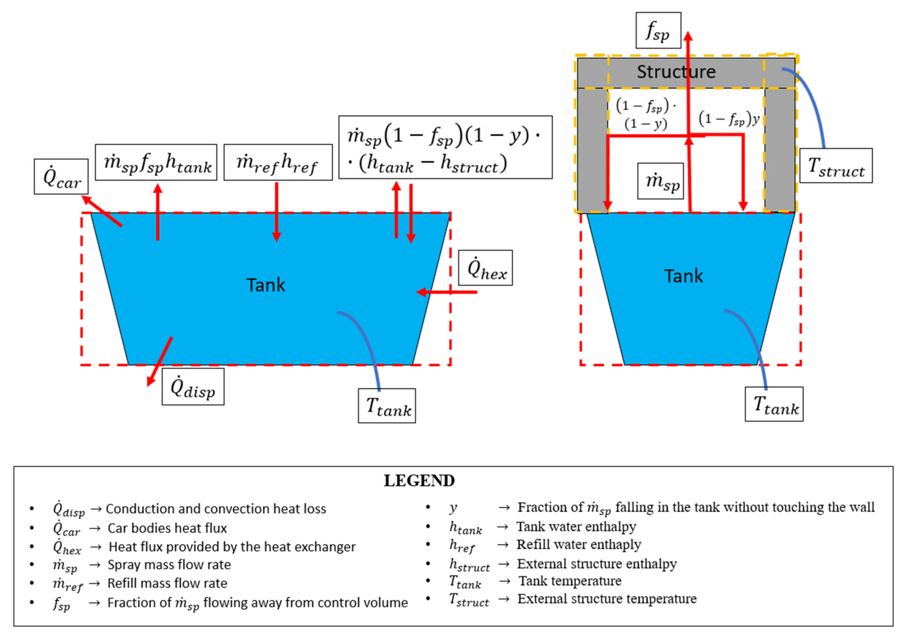
3.1. Mechanistic Physics-Based Model Approach

The physics-based thermodynamic approach relies on the evaluation of all the heat losses of the degreasing process based on physical relationships. In Figure 2, a schematic representation of the degreasing tank is provided, indicating the control volumes for the water volume in red, the external tunnel structure in yellow, and of all the heat losses considered in the model.
The term Q ˙ d i s p refers to the conduction and convection heat losses with the external environment, whereas the term Q ˙ c a r is associated with the heat flux provided to heat the car bodies. Regarding the spray dispersion terms, we assumed that the entire spray mass flow rate m ˙ s p is divided into two distinct contributions: one that flows away from the red control volume (the fraction of which is indicated by f s p in the figure above) and the other that falls back into the tank ( 1 f s p ). At this point, for the contribution of the not-dispersed mass flow rate, we assumed that a portion of it falls directly back into the storage tank without touching the walls of the external structure (the fraction of which is indicated by y in the figure above), resulting in a neutral contribution in terms of dispersions. Conversely, the remaining fraction ( 1 y ) falls back into the water tank only after coming into contact with the walls of the external structure, assuming the water temperature is the same as that of the structure itself. To account for the different behavior of the spray mass flow rate impacting the tunnel structure walls based on whether a car body is in the process or not, two distinct y coefficients were considered: y 1 in case of the absence of car bodies in the degreasing tank, and y 2 in case of their presence. The term m ˙ r e f · h r e f represents the refill contribution required to maintain a constant water level in the tank, while Q ˙ h e x is the heat flux term provided by the external heat exchanger in order to compensate for all the dispersion terms and the contribution needed for the tank water heating.
Taking all these factors into account, the mass and energy equations for all the control volumes can be written as follows:
d m w d θ = m ˙ r e f m ˙ s p · f s p
m w θ · c w · d T t a n k d θ = Q ˙ h e x Q ˙ c a r Q ˙ d i s p m ˙ r e f c r e f T t a n k T r e f m ˙ s p 1 f s p 1 y c s p T t a n k T s t r u c t
m c s t r u c t · d T s t r u c t d θ = m ˙ s p 1 f s p 1 y c s p T t a n k T s t r u c t
Equation (1) represents the mass balance for the water tank (red control volume in the figure above), and establishes a connection between the water mass variations ( m w ) and the inlet (refill, m ˙ r e f ) and outlet (spray dispersions, m ˙ s p · f s p ) mass flow rates. Equation (2) represents the energy balance for the same control volume, and it expresses the tank temperature ( T t a n k ) variation as a function of the dispersion terms previously described. Lastly, Equation (3) is the energy balance for the external tunnel structure (yellow control volume) aimed at evaluating the structure temperature ( T s t r u c t ) variation as a function of the spray contribution, which directly impacts the internal tunnel walls.
Each of the terms of Equations (1)–(3) was evaluated as follows. For the heat exchanger contribution, an energy balance on the primary hot water line mass flux was conducted.
Q ˙ h e x = m ˙ w , h e x · c w , h e x · T i n , h e x T o u t ,   h e x
Concerning the contribution from the car bodies, it was assumed that the entire body starts at the same temperature as the external environment and heats up to match the same temperature of the tank. The term Δ θ c a r represents the duration for which the car body remains inside the tank.
Q ˙ c a r = m c a r · c c a r · T t a n k T a m b Δ θ c a r
In this way, an average thermal power for the cars contribution was considered over the entire cycle time for each car body. This approach was the only feasible option given the available data provided by the production plant. Conversely, the refill contribution was evaluated as follows:
Q ˙ r e f = m ˙ r e f c r e f T t a n k T r e f
Regarding the heat losses contribution with the external environment, it was evaluated for the entire external surface of the degreasing tank by considering an average global conductance U m e a n , as follows:
Q ˙ d i s p = U m e a n · A t a n k · T t a n k T a m b  
Finally, the dispersion contribution related to the spray was calculated using the following expression.
Q ˙ s p = m ˙ s p 1 f s p 1 y c s p T t a n k T s t r u c t
The terms f s p and y were previously defined above.
Most of the temperature and mass flow rate terms in Equations (1)–(3) were directly measured though a dedicated sensor suite installed on the machine. The thermodynamic properties of water, such as density and specific heat, were assumed to be constant, whereas other properties of the car bodies (mass, specific heat) were obtained from datasheets provided by the plant. Conversely, all the unknown terms of Equations (1)–(3), including U m e a n , y1, y2, m c s t r u c t , and f s p were calibrated using experimental data, as shown in Section 4.1.

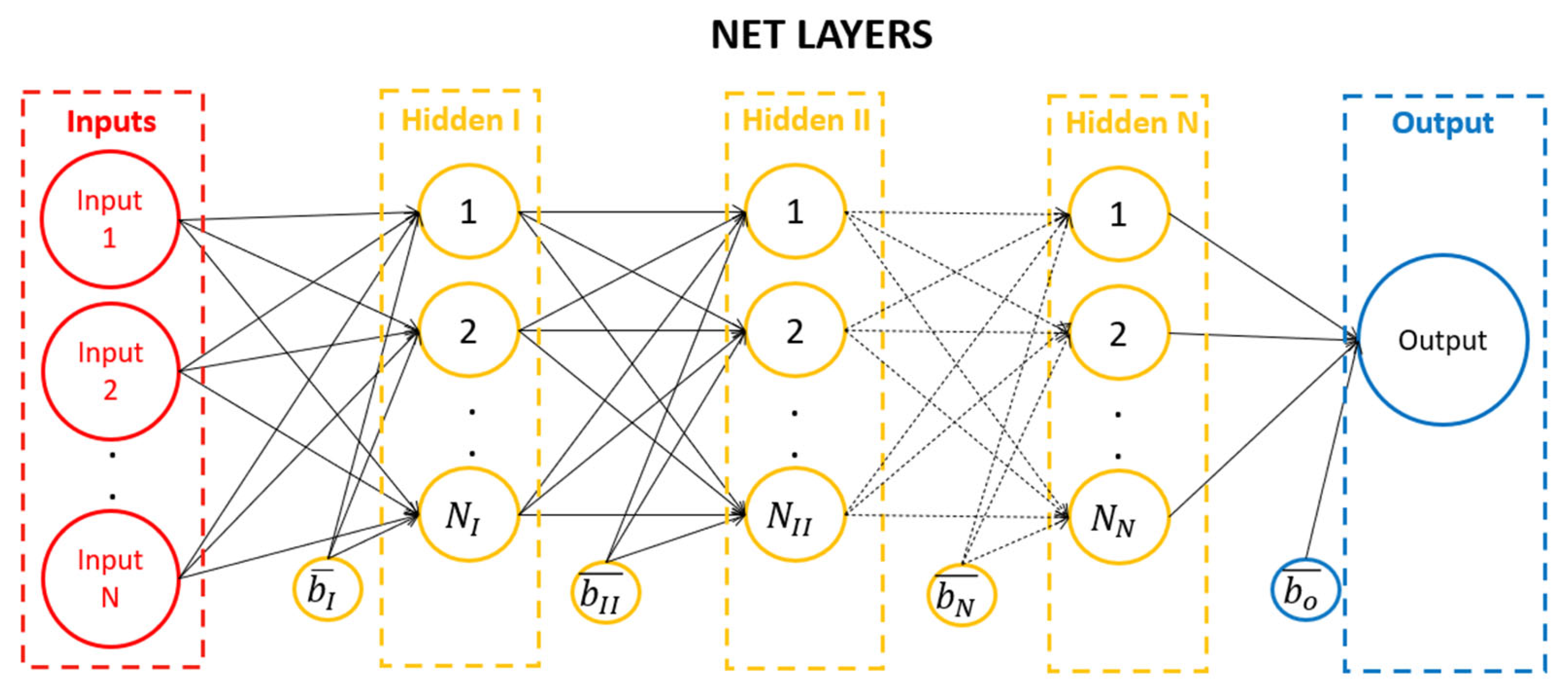
3.2. Artificial Neural Network (ANN) Model Approach

In this study, artificial neural networks (ANNs) were developed and calibrated to predict the behavior of the analyzed case study. As is commonly known, there are numerous machine learning methods used to model thermodynamic processes, including classification algorithms (such as SVM, KNN, Naïve Bayes etc.) and regression tools (ANNs) [40]. ANNs were chosen because, compared to other common machine learning tools, they are the most frequently used due to their speed, simplicity, and ability to solve complex non-linear problems with differential equation systems, such as the one presented in this work [41,42]. A schematic for the developed ANNs is presented in Figure 3, comprising an input layer, one or more hidden layers, and one output layer, with each layer containing a certain number of neurons [43].
Each connection between two neurons belonging to two subsequent layers represents a weight, while each neuron serves as an activation function. Therefore, at the input of each layer, all of the output values derived from the previous layer and multiplied by the corresponding connection weight are summed [44], with the possible addition of an external bias. The result of this operation is then evaluated by a generic neuron through an activation function, determining the output value, which is then provided to the next layer. Among all the possible activation functions [45], the chosen one for all the hidden layers is a hyperbolic tangent. Consequently, the training phase of an artificial neural network consists of calibrating all the weights and biases though several iterations, referred to as epochs, in which the network attempts to predict the output values based on the available experimental data. The network is considered calibrated when it achieves a target value for the error (RMSE, MAE, or others) between the actual and predicted output values.
In detail, three different ANNs were calibrated and, from this point in the paper, they will be referred respectively as ANN 1 to 3. They each involve different input and output variables and structures. ANN 1 and ANN 2 share the same five inputs, which include the actual temperature of the tank, the presence of a car body in the tank, the status of sprays (on/off), the ambient temperature, and the heat exchanger thermal power. ANN 1 predicts the gradient of the tank temperature in a given time step (in °C/s), whereas ANN 2 directly predicts the value of the temperature at the subsequent time step. Lastly, ANN 3 considers both the actual and consecutive temperatures as inputs to predict the required thermal power to satisfy the assigned temperature gradient. Table 2 provides the main characteristics of the investigated ANNs, including the inputs, outputs, and the number of layers and of neurons per layer (ANN structure). The structure of each ANN (number of hidden layers, number of neurons) was chosen in order to ensure the best prevision accuracy for each selected input and output subset for each of the three investigated ANNs.
For the calibration process, the entire database for the used case was randomly divided into 70% for training, 15% for validation, and 15% for testing. A maximum number of 2000 epochs was selected, and the calibration was executed using a Levenberg–Marquardt algorithm [46,47] to minimize the mean squared errors between the target and predicted outputs.
Finally, validation was conducted on the entire database, as shown in the sections below.

4. Model Calibration and Validation

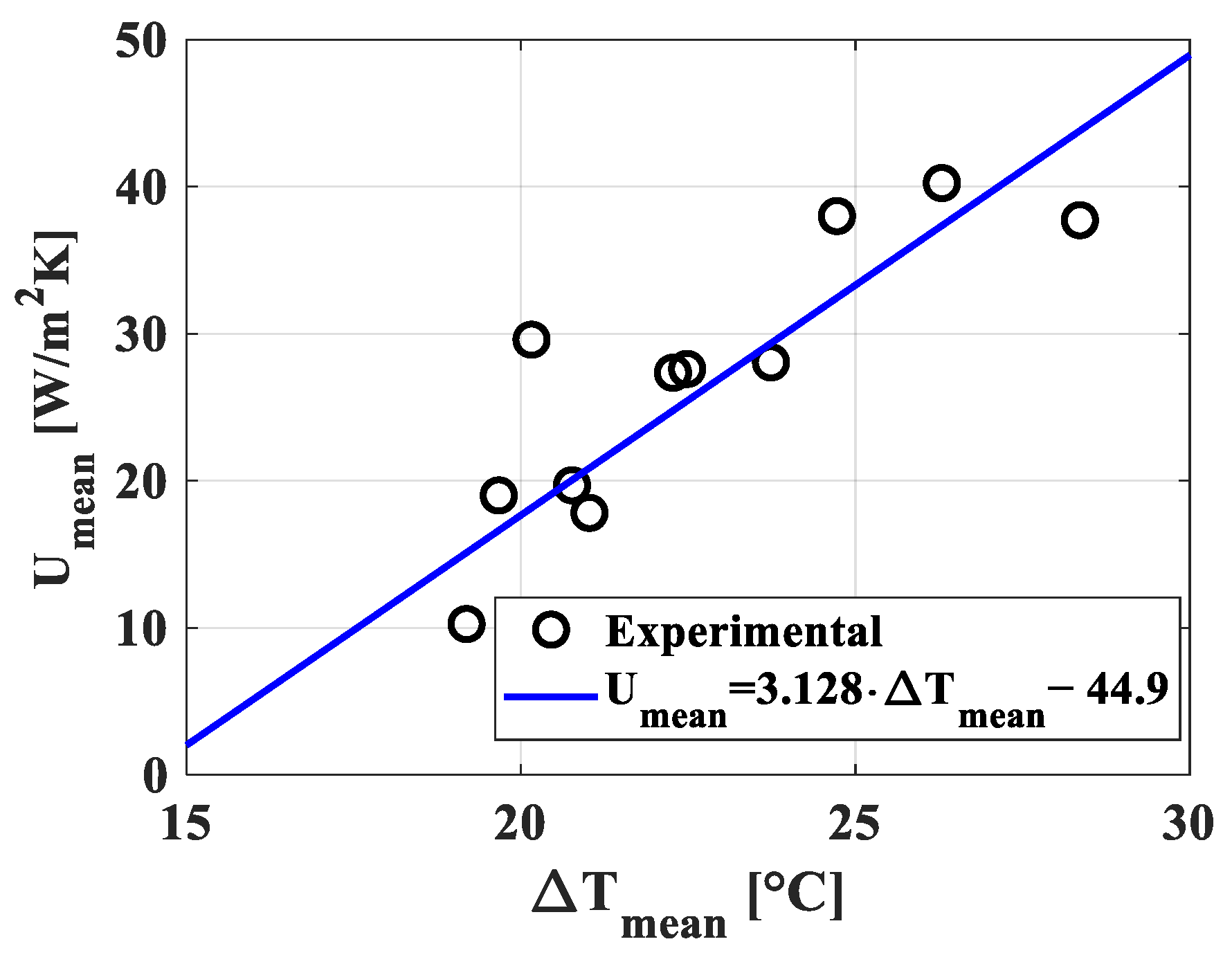
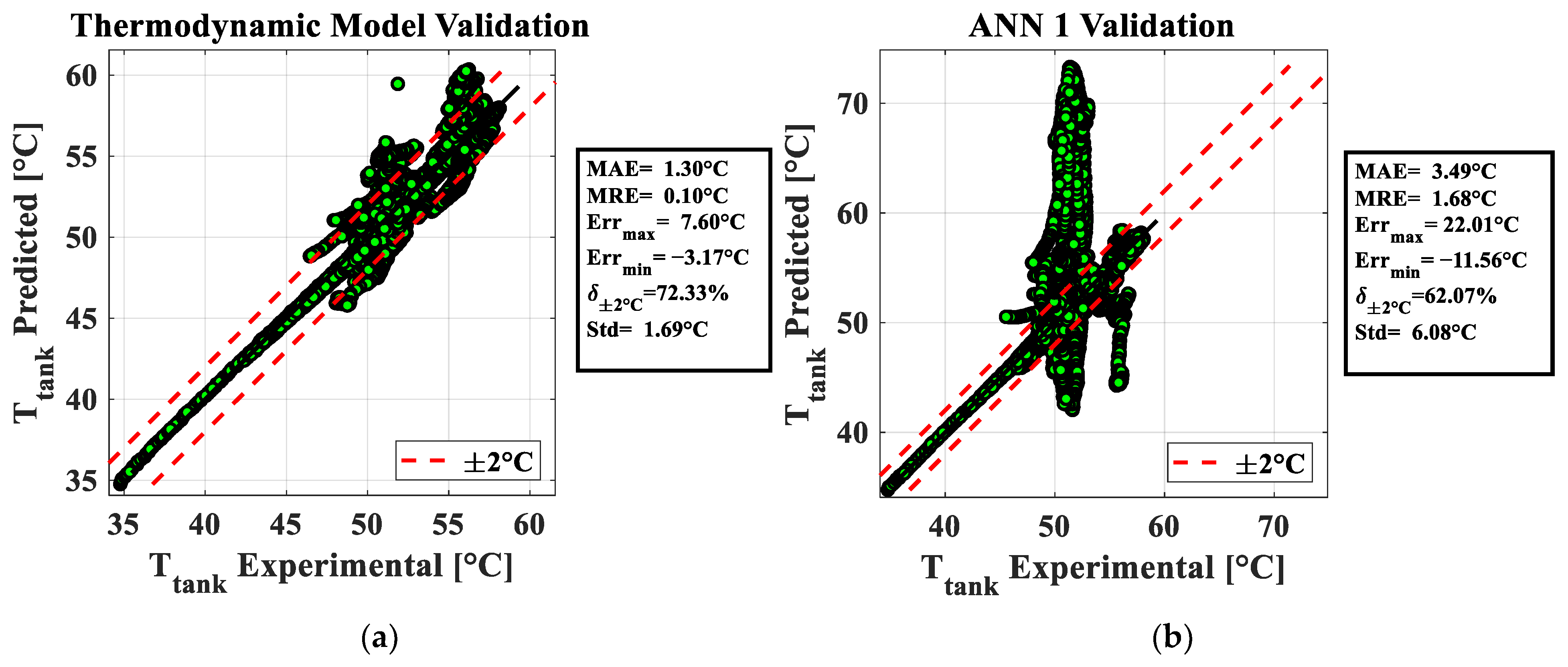
4.1. Thermodynamic Model Calibration and Validation

The average global conductance of the external walls ( U m e a n ) in Equation (7) was calibrated by analyzing the decreasing trend of the tank temperature for about 11 days using the experimental data of the case study. It can be demonstrated that when all of the terms of spray, refill, heat source, and car bodies in Equation (2) are absent, leaving only the heat losses with the external environment, the model can be simplified to the following equation:
d T T a m b T T a m b = U m e a n A t a n k m w c w d θ = 1 τ d θ
where τ is defined as τ = m w c w U m e a n A t a n k , m w is the mass of the water in the tank, and A t a n k is the lateral surface area of the container. This equation was integrated over the time period between the shutdown of the previous day and the startup the next day. This was carried out by isolating the experimental points in which the system was turned off, and all the energetic contributions, apart from the dispersions, were absent. Consequently, the values for the τ constant, and thus, for U m e a n , were determined considering the initial and final water tank and ambient temperatures for each of the 11 experimental tests.
τ = Δ θ ln T f T a m b , f T i T a m b , i U m e a n = m w c w τ A t a n k
Finally, a linear equation representing U m e a n as a function of the average temperature difference between the tank and the external ambient has been fitted, as shown in Figure 4.
U m e a n = 3.128 · T t a n k T a m b 44.9
Regarding the calibration for the contribution of the spray mass flow rate not returning into the tank ( f s p ), it was determined by calculating the ratio between the total mass of refilled water and the total mass of water injected by the sprays, as follows:
f s p = m ˙ w , r e f d θ m ˙ w , s p d θ
Finally, the three remaining coefficients y 1 , y 2 , and m c s t r u c t were similarly calibrated using the experimental data of the water tank temperature evolution through manual research, considering relatively large and plausible variation ranges for each variable to find the solution with the minimum mean absolute error (MAE) between the predicted and experimental water tank temperature profiles. The obtained values are reported in Table 3.
Figure 5 shows a comparison between the tank temperature evolution evaluated by the model (blue lines) and the experimental trend (red lines) for the charging process and the shift time period over six different working days throughout the year. Additional statistical parameters describing the prediction accuracy for each of these investigated days are provided in Table 4. These parameters included the mean relative error (MRE), the maximum ( E r r m a x ) and minimum ( E r r m i n ) errors, the percentage of point falling into the error band of ± 2   ° C ( δ ± 2   ° C ), and the standard deviation (Std) of the predictions. To address company confidentiality constraints, it should be noted that the work shift durations in all the subsequent figures were assumed to be equal for all the working days and different from the actual working time shift of the company.
It is important to highlight that the model consistently demonstrated the ability to predict the temperature trend during the initial heating period until the desired temperature setpoint was achieved. Moreover, on certain days (e.g., days 1, 3, and 4), the model exhibited good predictive capability even during steady-state conditions, with a mean absolute error (MAE) of less than or around 1 °C. On other days (e.g., days 2, 5, and 6) the model was still able to predict the experimental results at an early stage, before diverging due to less accurate estimations of some terms of the energy balance equation (Equation (2)). Nonetheless, the MAE during this phase remained below 2 °C, with a maximum errors staying under 5 °C. As a matter of fact, after the initial heating of the water within the tank, external factors started to influence the dispersion process, including the spray activation, the entering of the car bodies etc. Thus, during this phase, the model may lack accuracy, especially if one of these terms is badly predicted.

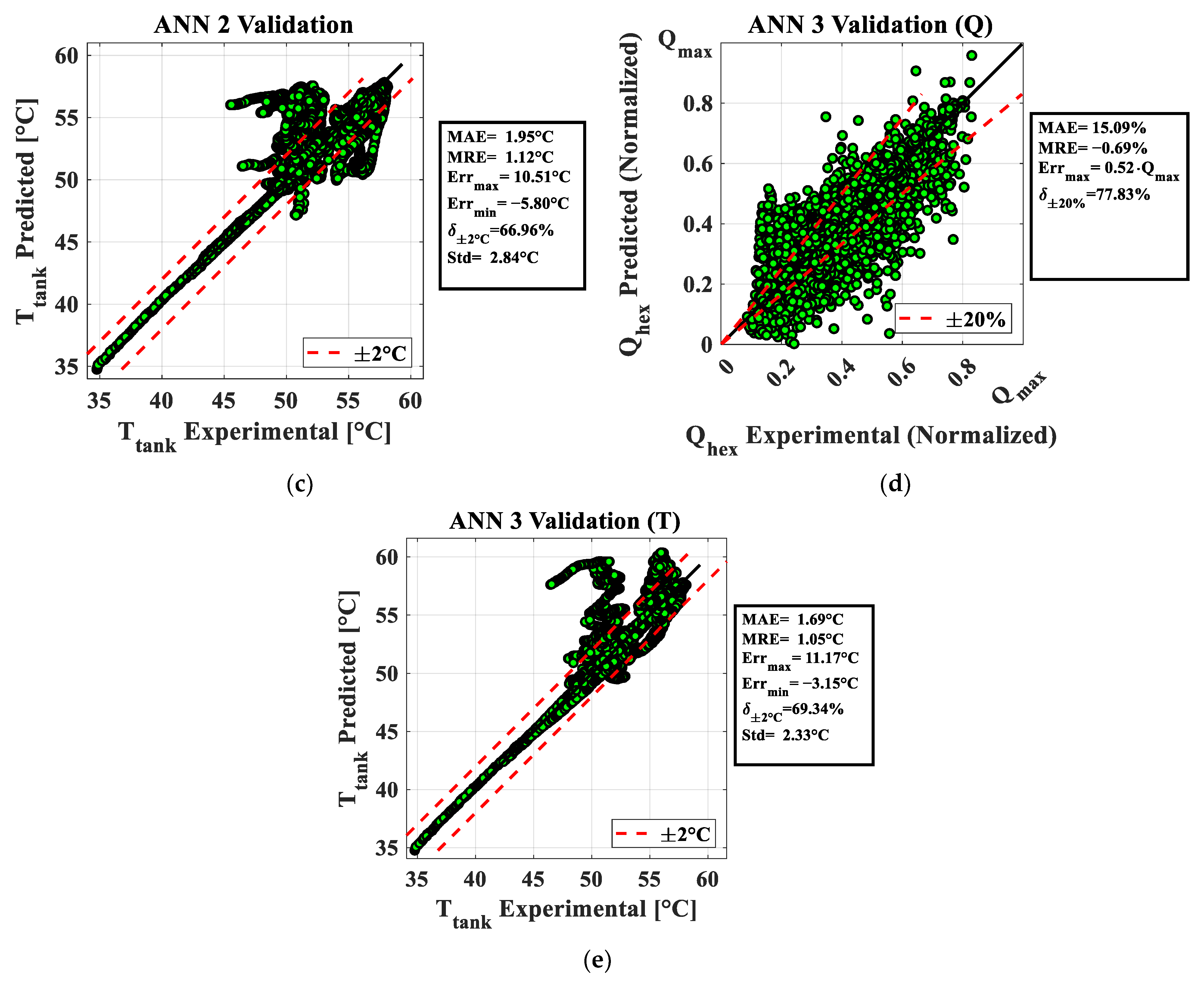
4.2. ANN Model Calibration and Validation

Each of the ANNs defined in Section 3.2 was calibrated using approximately 9000 experimental points from 13 working days of the production line. Similar to the thermodynamic physics-based approach, Figure 5 presents a comparison between the experimental results (red lines), the predictions made by ANN 1 (green lines), ANN 2 (magenta lines), and ANN 3 (cyan lines) in terms of the tank temperature evolution for six different working days. The statistical indexes of the prediction accuracy of all the methods are also provided in Table 4. It is worth noting that all the investigated ANNs, as well as the physics-based model, were quite able to predict the tank temperature evolution during the initial pre-heating phase with good accuracy. Moreover, for ANN 1, which predicted the temperature gradient of a specific time step as a function of several predefined input variables, it was observed that on some working days (e.g., days 5 and 6), the overall prediction accuracy was quite high, even better than that of the thermodynamic model. However, there were other days (e.g., days 2, 3, and 4) for which the ANN provided completely inaccurate predictions, with maximum errors exceeding 20 °C. For ANN 2, which directly predicted the tank temperature values in the subsequent timestep, there were no significant mispredictions compared to the experimental data, in contrast to ANN 1. On some days, the thermodynamic model seemed to perform better (e.g., days 3 and 4), while on other working days, the ANN model achieved higher prevision accuracy (e.g., days 1, 5, and 6). However, on day 2, the ANN initially predicted the experimental results well, before significantly diverging towards the end of the working shift. Finally, for ANN 3, which predicted the required thermal power for the heat exchanger based on the assigned temperature difference in a certain time step, similar results to the other ANNs were obtained. In fact, there were some days for which the neural network provided satisfactory results, and some others (e.g., day 1) for which the prediction was completely inaccurate. However, in this case, the tank temperature evolution was obtained by firstly calculating the thermal power using the calibrated ANN and then determining the temperature value by subtracting all the other heat losses evaluated by the relations in Section 3.1 from the HEX power.

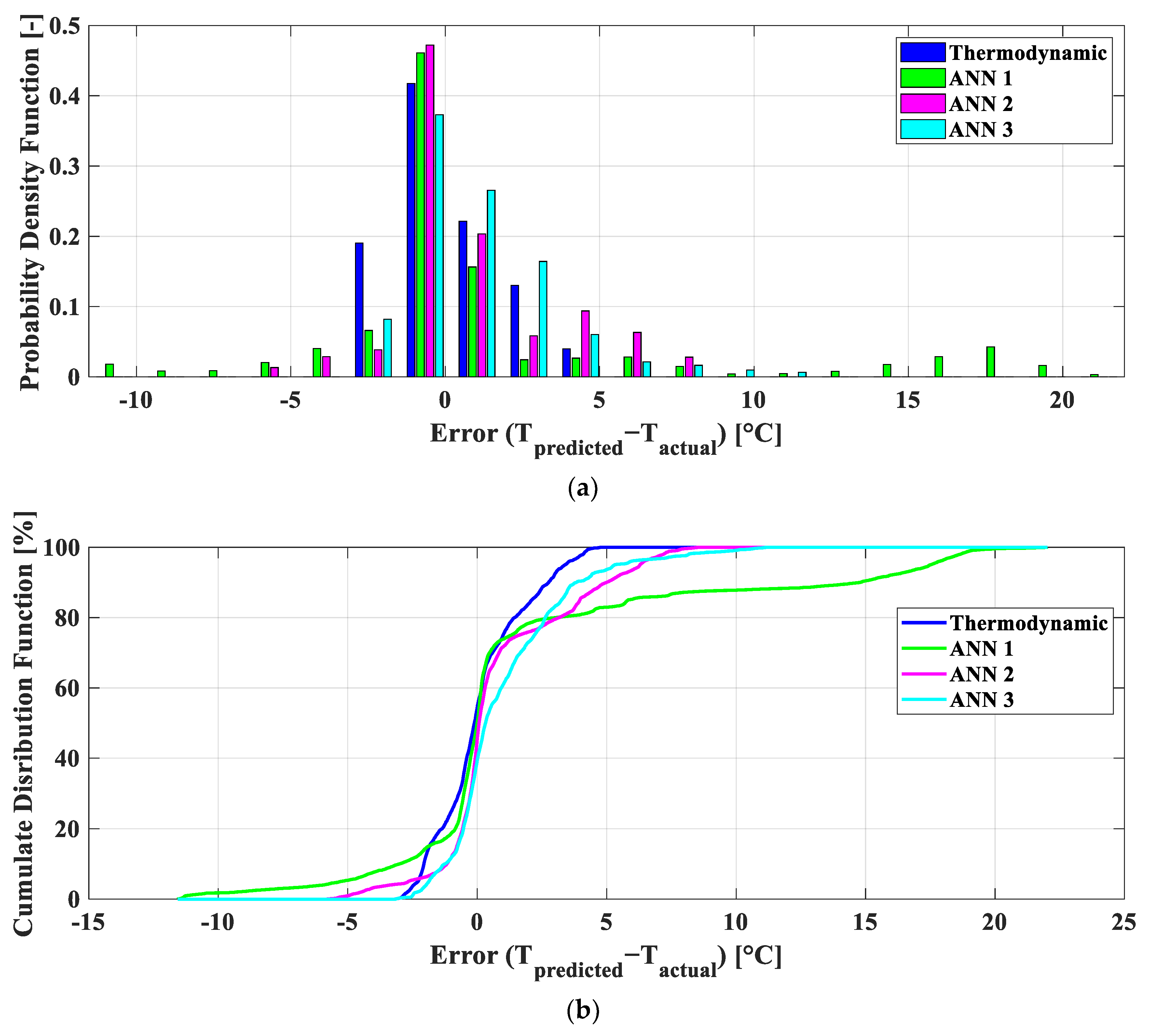
4.3. Summary of Prevision Accuracy of All the Modeling Approaches

A comprehensive statistical analysis was conducted over 13 production days (approximately 9000 experimental points) for all the investigated methods. Figure 6a shows a comparison between the tank temperature values predicted by the physics-based model and the experiment. As previously mentioned, the model demonstrated the ability to predict the water temperature with good accuracy at the beginning of the charging phases (lower values), but some bigger mistakes occurred when maintaining the tank at a steady state around the target setpoint temperature. Nevertheless, the MAE obtained for all the experimental points, approximately 1.30 °C, remained within the acceptable bounds. Figure 6b–e shows the overall prediction accuracy of the ANNs in terms of the tank temperature. Specifically, Figure 6b,c shows the validation results of ANN 1 and ANN 2, respectively, and Figure 6e,f reports the validation results of ANN 3, both in terms of the HEX thermal power and the water tank temperature. Overall, for ANN 1, an MAE of 3.49 °C was obtained, with 62% of all the points falling within the error band of ± 2   ° C . However, the number of completely mistaken predictions was quite high, with a maximum absolute error of approximately 22 °C. ANN 2 achieved an MAE of 1.95 °C, with a maximum error of about 11 °C, which is lower compared to that of ANN 1. Finally, for ANN 3, the prediction on HEX thermal power was characterized by an MAE of 15%, with 78% of the points falling within the error band of ± 20 % . Regarding the tank temperature prediction, an MAE of approximately 1.7 °C was obtained, with 69% of the points falling within the error band of ± 2   ° C .
Figure 7 shows the probability density function (PDF, Figure 7a) and the cumulative distribution function (CDF, Figure 7b) of the error between the actual and predicted tank temperature values for all four models analyzed in this work. From Figure 7a, it is noteworthy that although ANN 1 and ANN 2 had the highest PDF, in close proximity to the zero, the thermodynamic model never reported absolute errors higher than 3–4 °C. In contrast, ANN 2 and ANN 3 gave errors exceeding 5 °C, and ANN 1 over 15 °C. This observation is further presented in Figure 7b, where the thermodynamic model has a CDF with the lowest deviation relative to the mean value compared to the other models, despite ANN 1 and ANN 2 having the steepest slopes closest to zero error.
Table 5 presents the global statistic indexes indicating the goodness of prevision for the degreasing tank temperature for each of the analyzed approaches. It is worth noting that the mechanistic physics-based model yielded the lowest values of MAE and MRE, followed by ANN 3 and ANN 2. In contrast, ANN 1 exhibited the lowest prediction accuracy, especially due to its tendency to make substantial mistakes (maximum error of approximately 22 °C).
Among the analyzed approaches, and based on the data at the disposal from the company, it appears that the thermodynamic approach was better suited for predicting the future behavior of the analyzed system. Regarding real-world implications, the use of a thermodynamic approach can guarantee results that are never completely wrong, thanks to the reliability on physical equations and principles. On the other hand, ANNs tend to produce higher errors, especially because of the nature of the problem. As a matter of fact, when a dynamic and continuous prediction is performed, the extrapolation mistake of the networks propagates into the future, strongly influencing all of the consecutive timestamps of the dynamic prevision and leading to significant inaccuracies in the ML methods. Moreover, the error differences among the three investigated ANNs may depend on the different structures of the inputs and outputs, which are more or less compatible with the chosen network architectures.
Finally, regarding the choice of modeling tool, the usage of one versus another approach has several advantages and limitations. A thermodynamic approach is well-suited when there are sufficient data to comprehensively describe all the physical aspects, and any information gaps can be partially compensated for by grey-box approaches, such as the one presented in this work, where the constant parameters can be finely tuned using experimental data. On the other hand, when dealing with incomplete data and missing sensors, ANNs can be more appropriate since they rely exclusively on historical data used for the training phase. However, in this case, it is essential to collect experimental data that cover a wide range of boundary conditions to minimize extrapolations which may lead to significant prediction errors. This cannot be always guaranteed due to the presence of some conditions that rarely occur in operating production plants, and which cannot be virtually experimented on due to production constraints in the manufacturing facility.
Overall, considering the reasons presented above, the thermodynamic approach was chosen to carry out the scheduling optimization, which is presented in the following sections.

5. Use of the Model for Optimization Strategies

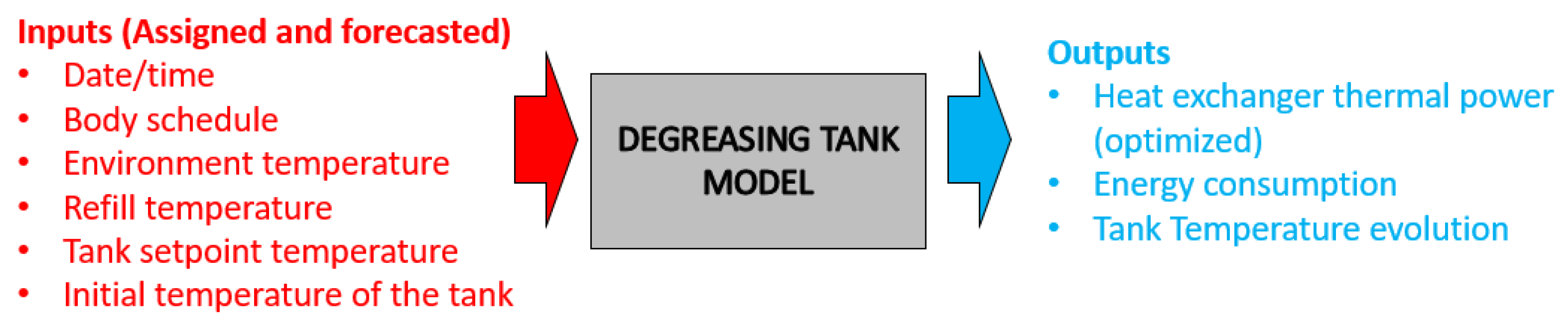
5.1. Usage of the Model in Simulation Mode and Assumptions

Among the developed models, the thermodynamic approach was selected to be used to carry out the optimization of the heat exchanger thermal power policy and to evaluate the energy consumption in each of the analyzed scenarios. Specifically, the main goal of this analysis is to provide for the model several input data of future production shifts, including the date/time, a hypothetical entering/exiting car body schedule, environmental and refill temperature conditions, the desired tank setpoint temperature, and the initial tank temperature. In return, the model gives, as output, the heat exchanger thermal power profile, the tank temperature evolution, and the total amount of energy consumed during the assumed car body scheduling. The complete input–output list for this phase is provided in Figure 8.
The following control logic of the system was assumed:
(1)
A constant rated value for the spray mass flow rate was assumed 1 min before the entrance of the first car body in the process. If no car body enters in 9 min during the process, the sprays are turned off.
(2)
The refill mass flow rate is maintained at a constant rated value to keep the water level within a certain a priori fixed dead-band.
(3)
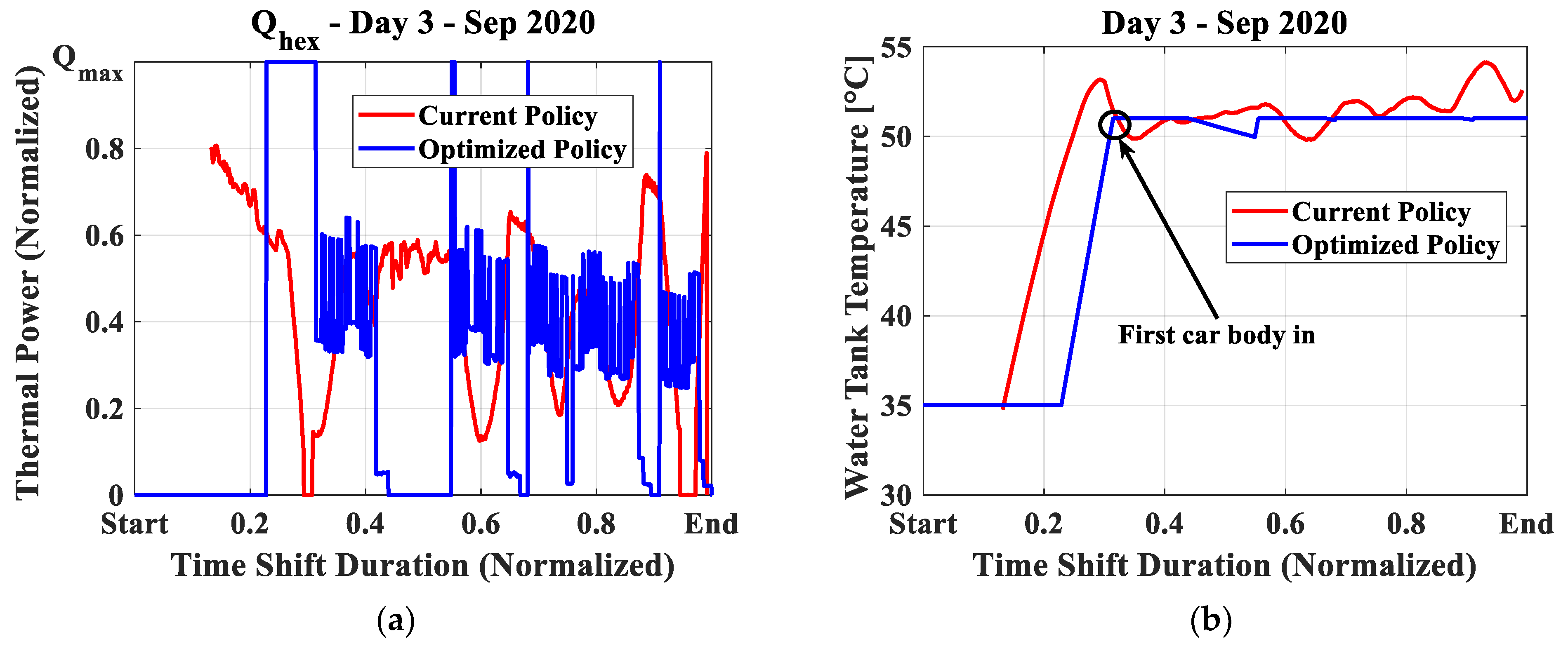
For the heat exchanger, the maximum thermal power ( Q ˙ m a x ) is imposed during a pre-heating stage to reach the desired setpoint temperature in the tank exactly when the first car body enters the process. If no car body enters in 30 min, the thermal power is turned off. The same logic is applied each time the heat exchanger is turned on.

5.2. Optimization with Real Data of the Case Study

In this section, a body schedule from a real production day is considered to demonstrate the utility of the model on real historical data. Specifically, a comparison between the actual and optimized policies was carried out to identify the optimal conditions and evaluate the effective energy saving of the optimized scenario compared to the current policy. The actual regulation is manual and based on the operator experience, whereas the optimized heat exchanger policy is the result of the simulation of the model. In Figure 9a the comparison between the current (red line) and optimized (yellow line) HEX thermal power policies is shown. Both the policies were normalized to the maximum value of the HEX thermal power for confidentiality reasons, along an entire time shift. Figure 9b shows the corresponding tank temperature values, and it can be seen that the optimized policy ensured that the tank temperature reached its setpoint value exactly when the first car body entered the process, avoiding unnecessary superheating of the water inside the tank. Moreover, after the preheating phase, the model provided the exact thermal power policy needed to maintain the tank at the desired setpoint value, reducing the fluctuations observed in the current manual regulation.
Finally, the energy consumption throughout the entire time shift, normalized for the energy consumption of the current policy for confidentiality reasons, is reported in Figure 10. With the optimized policies generated by the digital model, it is evident that there would be an energy saving of about 31% for the investigated working day.

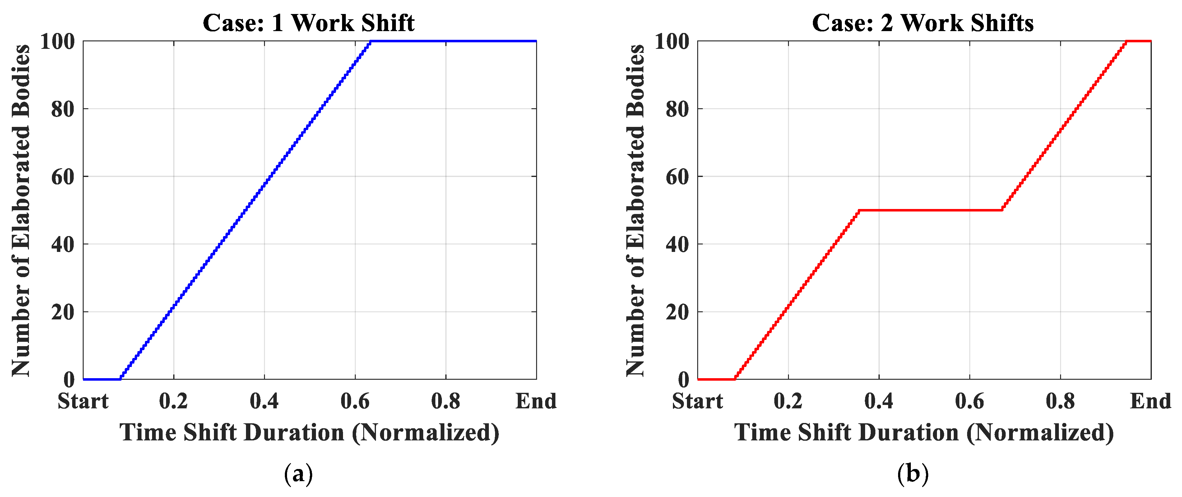
5.3. Optimization with New Body Schedule

An example of the usage of the model with the aim of optimizing a new hypothetical body schedule is presented in this section. Particularly, we considered the production of 100 car bodies in two different scenarios: one where the production occurs in a single work shift, and another where it is split into two different work shifts. Obviously, to minimize heat losses and dispersion with the external environment, the ideal solution would be to process the entire batch as quickly as possible. However, this may not always be feasible due to various company constraints. It is important to note that there could be some company restrictions regarding the duration of work shifts, as well as potential interruptions to the production due to scheduled maintenance operations or equipment failures. Therefore, using the model, the extra energy consumption of every simulated scenario, which differs for several reasons from the optimal one, can be estimated.
The following input and cycle data were fixed:
(1)
Each car body must remain in the degreasing tank for a minimum of 3 min, and there is a 1 min waiting time between the entry of two consecutive car bodies in the process.
(2)
A setpoint temperature of 50 °C was considered, with an initial temperature of the tank of 30 °C.
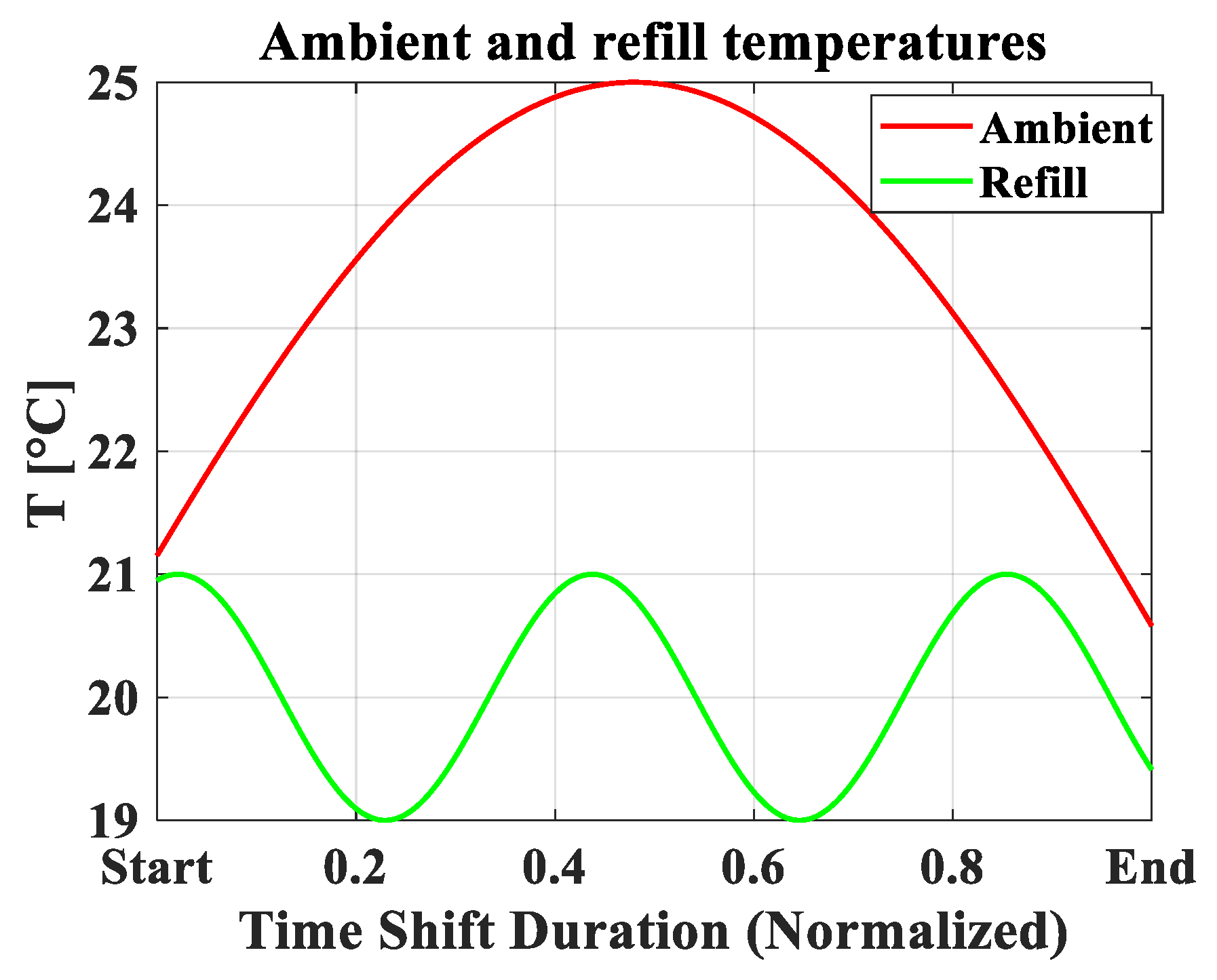
(3)
The ambient and refill temperature trends shown in Figure 11 were determined. It should be clarified that all the input data were chosen solely for the purpose of the results and optimization in this paper, and they do not represent real data on the effective production processes of a company.
The first of the two cases analyzed was a scenario with a single work shift, where the first car body must enter the process at the normalized time 0.1 of the total daily work shift (from start to end of the figure above). The second case, on the other hand, involves a scenario with two work shifts, in which the entire production is divided equally, the first from time 0.1 to 0.35 and the second from time 0.65 to the end of the total daily work shift. Figure 12 illustrates the body schedule in terms of the cumulative number of processed bodies for both the single work shift (Figure 12a) and the two work shift (Figure 12b) scenarios.
Figure 13 presents the results of the HEX thermal powers (Figure 13a), tank temperatures (Figure 13b), and energy consumed (Figure 13c) for the two analyzed scenarios. To account for the communication time delays between the sensor suite and valve actuation, related to the system inertia and other factors, a 15-min moving average was applied to the thermal power. It is worth noting that, in order to achieve the desired temperature right at the entrance of the first car body (at normalized time 0.1), the system should be turned on at approximately the beginning of the work shift. Moreover, in the first case, the complete production ended at about a normalized time of 0.61, whereas in the second case, the system was turned off at approximately 0.4, and re-turned on at 0.64 to achieve the desired setpoint temperature right at the entrance of the first body in the second work shift (normalized time of 0.65). Finally, regarding energy consumption, Figure 13c shows that considering a two work shift scenario led to an extra energy consumption of approximately 9% compared to the one work shift case.

6. Conclusions and Future Developments

This paper presents the development of a model for predicting the temperature evolution and energy consumption of a degreasing tank in an automotive production process, which is a preliminary phase of the painting of car bodies. Such a predictive model that is able to predict the future behavior of this process would be significantly useful, both in terms of optimizing the energy consumption and the control of the system, and to re-schedule manufacturing in case of sudden machine stops, changes in production, maintenance operations, etc. The primary objective of this study was to carry out an assessment and comparison of different modeling approaches and to employ the most effective model for optimizing the heat source policy and analyzing future scenarios involving various production schedules. The key findings and outcomes are provided here:
  • Two distinct modeling approaches are presented: a thermodynamic physics-based approach that relies on mass and energy balances of different control volumes of the degreasing tank, and a machine learning approach consisting of three ANNs characterized by different structures, numbers, and typology of inputs and outputs.
  • Both modeling approaches were evaluated and compared with the experimental data obtained from a case study of an automotive production facility. For the thermodynamic model, several empirical variables, which cannot be deduced from the case study data, were calibrated using approximately 9000 experimental points. In contrast, the ANNs were calibrated by splitting the whole dataset into subsets for training, validation, and testing purposes.
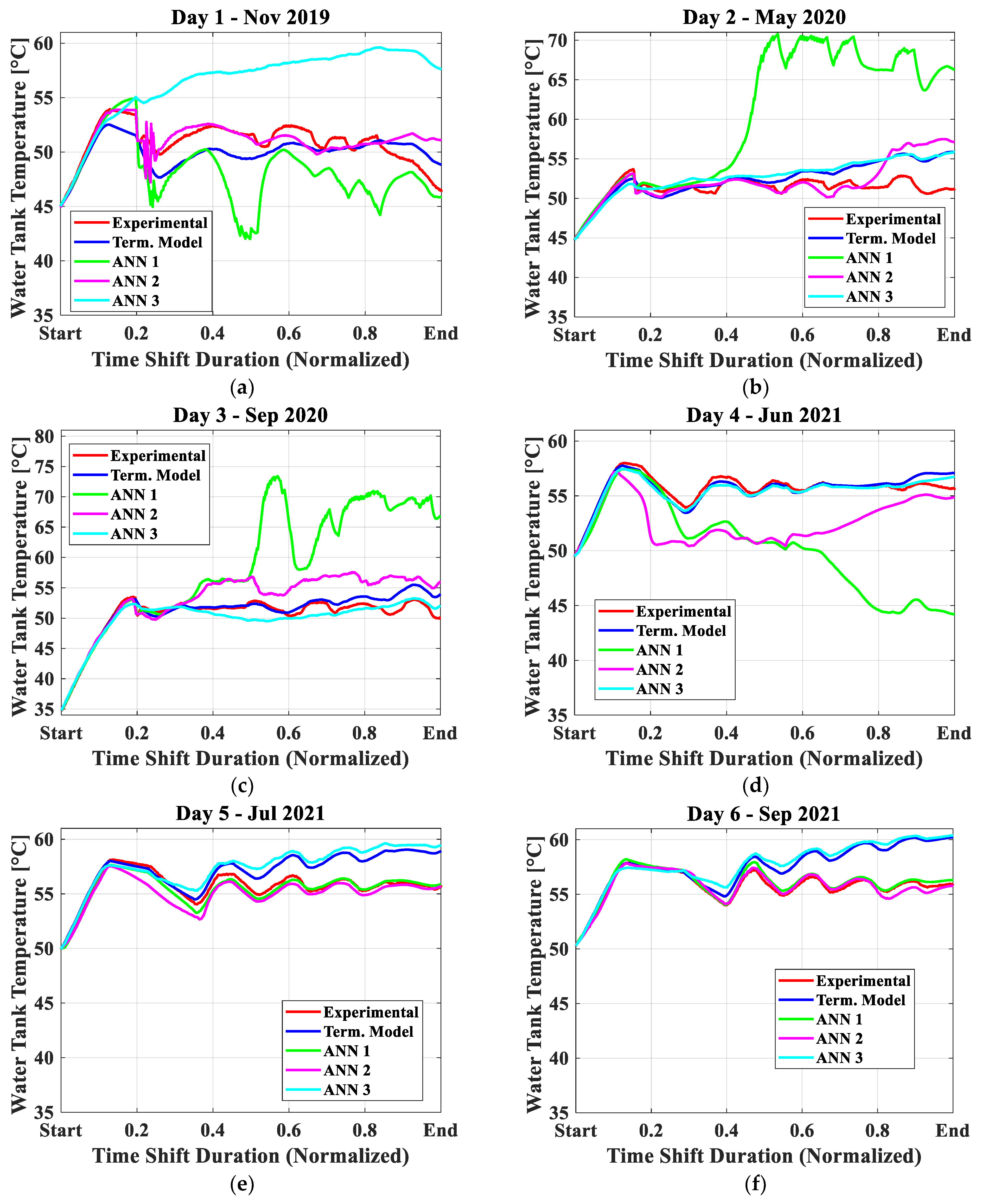
  • The results indicate that, for the analyzed case study, the thermodynamic model exhibited higher prediction accuracy for the tank temperature future trend, achieving an MAE of 1.36 due to all the information from the real data of the company. In contrast, all the ANN approaches exhibited higher MAEs and maximum errors, ranging from 10 to 22 °C, and posing a risk of completely inaccurate predictions.
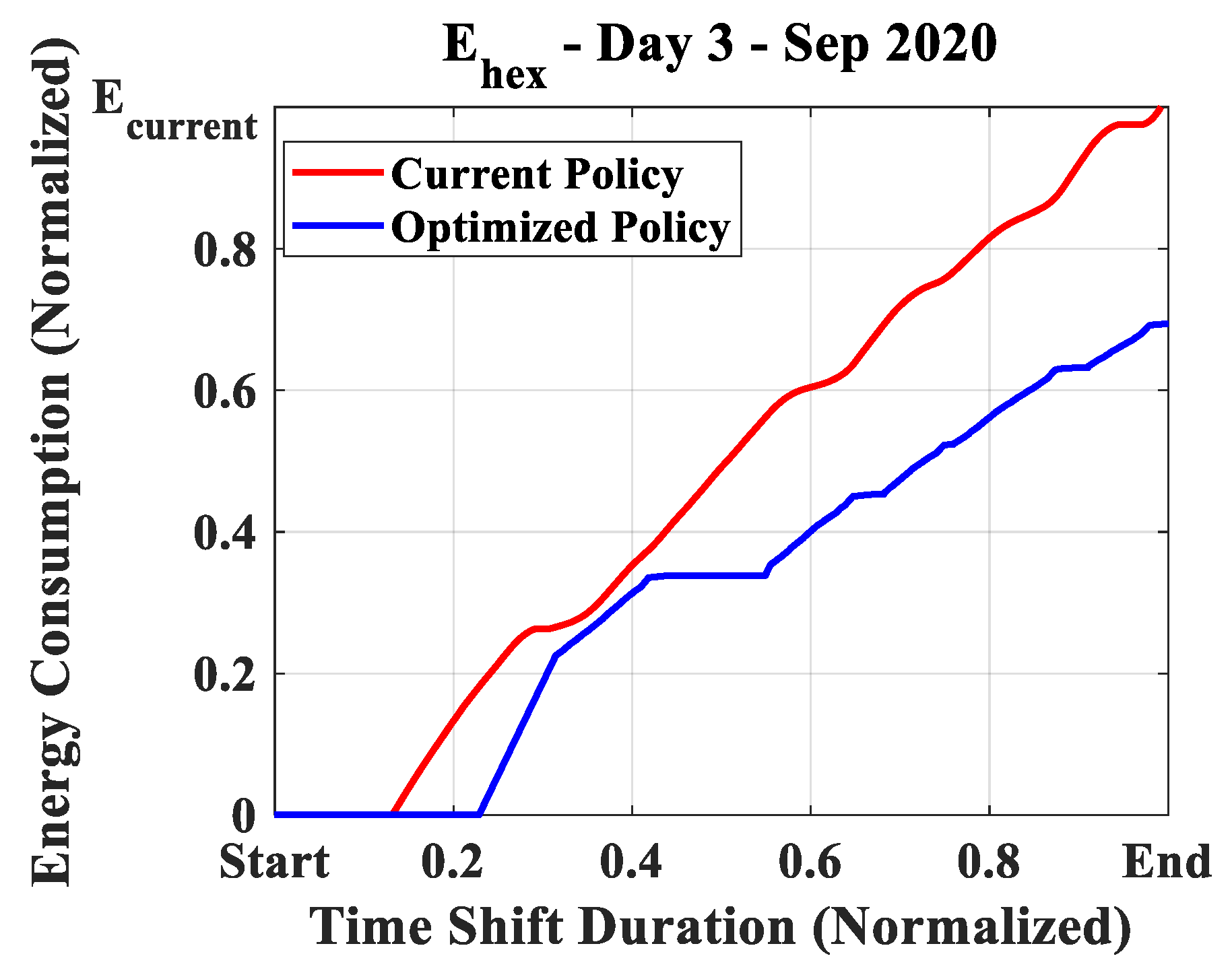
  • The thermodynamic approach was subsequently used to optimize the production process. Based on historical data for a working production day, employing an optimize heat load profile policy recommended by the model could lead to an energy saving of approximately 31% by limiting useless superheating of the water inside the tank and by limiting fluctuations around the desired setpoint value.
  • Considering a supposed production of 100 car bodies, the study explored two hypothetical future production scenarios, the first in which the production is performed in a single work shift, and the second in which the production is divided into two work shifts, potentially due to company constraints or planned maintenance operations. In this case, the model was able to provide an estimation of the extra energy consumption of the second scenario compared to the first, which was approximately 9%.
In conclusion, as part of the EnerMan Project [38], this study demonstrates that the development of predictive models for a degreasing tank in automotive production and their implementation into an optimizer would achieve substantial energy savings of up to 20–30%. This approach can also be applied in other applications in which a careful temperature control of a water tank is needed, beyond the automotive sector (e.g., chemical industry, swimming pools, etc.). Moreover, within the framework of the EnerMan Project [38], other case studies in the automotive sector that could benefit from a predictive model have been analyzed. Future developments will explore these applications to study the potentialities of this kind of approach in terms of energy saving.

Author Contributions

Conceptualization, A.W.M. and S.P.; methodology, A.W.M.; software, F.P.; validation, F.P. and F.M.; formal analysis, L.V.; investigation, F.P.; resources, A.W.M., S.P. and N.B.; data curation, F.P.; writing—original draft preparation, F.P.; writing—review and editing, L.V.; visualization, F.P.; supervision, A.W.M.; project administration, N.B. and A.Z.; funding acquisition, N.B. and A.Z. All authors have read and agreed to the published version of the manuscript.

Funding

This research was funded by the Energy-Efficient Manufacturing System Management (EnerMan) European Project, under Grant Agreement No. 958478.

Data Availability Statement

The data presented in this study are available upon request from the corresponding author. The data are not publicly available due to confidentiality issues of the owner company.

Acknowledgments

This research work was carried out as part of the Energy-Efficient Manufacturing System Management (EnerMan) Project founded by the European Union’s Horizon 2020 Program (Grant Agreement No. 958478).

Conflicts of Interest

We wish to confirm that there are no known conflicts of interest associated with this publication and there has been no significant financial support for this work that could have influenced its outcome. We confirm that the manuscript has been read and approved by all named authors and that there are no other persons who satisfied the criteria for authorship but are not listed. We further confirm that the order of authors listed in the manuscript has been approved by all of us. We confirm that we have given due consideration to the protection of intellectual property associated with this work and that there are no impediments to publication, including the timing of publication, with respect to intellectual property. In so doing, we confirm that we have followed the regulations of our institutions concerning intellectual property. We understand that the Corresponding Author is the sole contact for the Editorial process (including the Editorial Manager and direct communications with the office). He is responsible for communicating with the other authors about the progress, submissions of revisions, and final approval of proofs. We confirm that we have provided a current, correct email address that is accessible by the Corresponding Author.

References

  1. IEA. Industry; IEA: Paris, France, 2022; Available online: https://www.iea.org/reports/industry (accessed on 27 July 2023).
  2. IEA. Net Zero by 2050, IEA, Paris. 2021. Available online: https://www.iea.org/reports/net-zero-by-2050 (accessed on 27 July 2023).
  3. Driving the Motor Industry, 2020 UK Automotive Sustainability Report, 21st ed.; SMMT: London, UK, 2019.
  4. ANFIA (Associazione Nazionale Filiera Industria Automobilistica). Statistical Data, New Car Registration. Available online: https://www.anfia.it/it/dati-statistici/immatricolazioni-italia (accessed on 15 July 2023).
  5. Giampieri, A.; Ling-Chin, J.; Ma, Z.; Smallbone, A.; Roskilly, A.P. A review of the current automotive manufacturing practice from an energy perspective. Appl. Energy 2020, 261, 114074. [Google Scholar] [CrossRef]
  6. Biesinger, F.; Kraß, B.; Weyrich, M. A survey on the necessity for a digital twin of production in the automotive industry. In Proceedings of the 23rd International Conference on Mechatronics Technology (ICMT), Salerno, Italy, 23–26 October 2019; pp. 1–8. [Google Scholar]
  7. Afram, A.; Janabi-Sharifi, F.; Fung, A.S.; Raahemifar, K. Artificial neural network (ANN) based model predictive control (MPC) and optimization of HVAC systems: A state of the art review and casestudy of a residential HVAC system. Energy Build. 2017, 141, 96–113. [Google Scholar] [CrossRef]
  8. Afram, A.; Janabi-Sharifi, F. Review of modeling methods for HVAC systems. Appl. Therm. Eng. 2014, 67, 507–519. [Google Scholar] [CrossRef]
  9. Forbes, M.G.; Patwardhan, R.S.; Hamadah, H.; Gopaluni, R.B. Model predictive control in industry: Challenges and opportunities. IFAC-PapersOnLine 2015, 48, 531–538. [Google Scholar] [CrossRef]
  10. Narciso, D.A.; Martins, F.G. Application of machine learning tools for energy efficiency in industry: A review. Energy Rep. 2020, 6, 1181–1199. [Google Scholar] [CrossRef]
  11. Hu, Y.; Man, Y. Energy consumption and carbon emissions forecasting for industrial processes: Status, challenges and perspectives. Renew. Sustain. Energy Rev. 2023, 182, 113405. [Google Scholar] [CrossRef]
  12. Ascione, F.; Bianco, N.; Iovane, T.; Mauro, G.M.; Napolitano, D.F.; Ruggiano, A.; Viscido, L. A real industrial building: Modeling, calibration and Pareto optimization of energy retrofit. J. Build. Eng. 2020, 29, 101186. [Google Scholar] [CrossRef]
  13. Kapp, S.; Choi, J.K.; Hong, T. Predicting industrial building energy consumption with statistical and machine-learning models informed by physical system parameters. Renew. Sustain. Energy Rev. 2023, 172, 113045. [Google Scholar] [CrossRef]
  14. Aruta, G.; Ascione, F.; Bianco, N.; Mauro, G.M.; Vanoli, G.P. Optimizing heating operation via GA-and ANN-based model predictive control: Concept for a real nearly-zero energy building. Energy Build. 2023, 292, 113139. [Google Scholar] [CrossRef]
  15. Široký, J.; Oldewurtel, F.; Cigler, J.; Prívara, S. Experimental analysis of model predictive control for an energy efficient building heating system. Appl. Energy 2011, 88, 3079–3087. [Google Scholar] [CrossRef]
  16. Son, Y.H.; Park, K.T.; Lee, D.; Jeon, S.W.; Do Noh, S. Digital twin–based cyber-physical system for automotive body production lines. Int. J. Adv. Manuf. Technol. 2021, 115, 291–310. [Google Scholar] [CrossRef]
  17. Mendi, A.F. A Digital Twin Case Study on Automotive Production Line. Sensors 2022, 22, 6963. [Google Scholar] [CrossRef] [PubMed]
  18. Zhang, M.; Zuo, Y.; Tao, F. Equipment energy consumption management in digital twin shop-floor: A framework and potential applications. In Proceedings of the 15th International Conference on Networking, Sensing and Control (ICNSC), Zhuhai, China, 27–29 March 2018; pp. 1–5. [Google Scholar]
  19. Zhang, H.; Qi, Q.; Tao, F. A multi-scale modeling method for digital twin shop-floor. J. Manuf. Syst. 2022, 62, 417–428. [Google Scholar] [CrossRef]
  20. Zhang, H.; Liu, Q.; Chen, X.; Zhang, D.; Leng, J. A digital twin-based approach for designing and multi-objective optimization of hollow glass production line. IEEE Access 2017, 5, 26901–26911. [Google Scholar] [CrossRef]
  21. Min, Q.; Lu, Y.; Liu, Z.; Su, C.; Wang, B. Machine learning based digital twin framework for production optimization in petrochemical industry. Int. J. Inf. Manag. 2019, 49, 502–519. [Google Scholar] [CrossRef]
  22. Karanjkar, N.; Joglekar, A.; Mohanty, S.; Prabhu, V.; Raghunath, D.; Sundaresan, R. Digital twin for energy optimization in an SMT-PCB assembly line. In Proceedings of the IEEE International Conference on Internet of Things and Intelligence System, Bali, Indonesia, 1–3 November 2018; pp. 85–89. [Google Scholar]
  23. Çamdali, Ü.; Tunc, M. Steady state heat transfer of ladle furnace during steel production process. J. Iron Steel Res. Int. 2006, 13, 18–25. [Google Scholar] [CrossRef]
  24. Laha, D.; Ren, Y.; Suganthan, P.N. Modeling of steelmaking process with effective machine learning techniques. Expert Syst. Appl. 2015, 42, 4687–4696. [Google Scholar] [CrossRef]
  25. Paryanto, P.; Brossog, M.; Bornschlegl, M.; Franke, J. Reducing the energy consumption of industrial robots in manufacturing systems. Int. J. Adv. Manuf. Technol. 2015, 78, 1315–1328. [Google Scholar] [CrossRef]
  26. Atmaca, A.; Kanoglu, M. Reducing energy consumption of a raw mill in cement industry. Energy 2012, 42, 261–269. [Google Scholar] [CrossRef]
  27. Sanz, E.; Blesa, J.; Puig, V. BiDrac Industry 4.0 framework: Application to an automotive paint shop process. Control Eng. Pract. 2021, 109, 104757. [Google Scholar] [CrossRef]
  28. Zheng, Y.; Chen, L.; Lu, X.; Sen, Y.; Cheng, H. Digital twin for geometric feature online inspection system of car body-in-white. Int. J. Comput. Integr. Manuf. 2021, 34, 752–763. [Google Scholar] [CrossRef]
  29. Tharma, R.; Winter, R.; Eigner, M. An approach for the implementation of the digital twin in the automotive wiring harness field. In Proceedings of the 15th International Design Conference, Dubrovnik, Croatia, 21–24 May 2018; pp. 3023–3032. [Google Scholar]
  30. Li, W.; Kara, S. An empirical model for predicting energy consumption of manufacturing processes: A case of turning process. Proc. Inst. Mech. Eng. Part B J. Eng. Manuf. 2011, 225, 1636–1646. [Google Scholar] [CrossRef]
  31. Kara, S.; Li, W. Unit process energy consumption models for material removal processes. CIRP Ann. 2011, 60, 37–40. [Google Scholar] [CrossRef]
  32. Ma, Z.; Gao, M.; Wang, Q.; Wang, N.; Li, L.; Liu, C.; Liu, Z. Energy consumption distribution and optimization of additive manufacturing. Int. J. Adv. Manuf. Technol. 2021, 116, 3377–3390. [Google Scholar] [CrossRef]
  33. Corinaldesi, C.; Schwabeneder, D.; Lettner, G.; Auer, H. A rolling horizon approach for real-time trading and portfolio optimization of end-user flexibilities. Sustain. Energy Grids Netw. 2020, 24, 100392. [Google Scholar] [CrossRef]
  34. Saidu, M.M.; Hall, S.G.; Kolar, P.; Schramm, R.; Davis, T. Efficient Temperature Control in Recirculating Aquaculture Tanks. Appl. Eng. Agric. 2012, 28, 161–167. [Google Scholar] [CrossRef]
  35. Seung-Hwan, Y.; Jin-Yong, C.; Sang-Hyun, L.; Yun-Gyeong, O.; Koun, Y.D. Climate change impacts on water storage requirements of an agricultural reservoir considering changes in land use and rice growing season in Korea. Agric. Water Manag. 2013, 117, 43–54. [Google Scholar] [CrossRef]
  36. Zhao, J.; Lyu, L.; Han, X. Operation regulation analysis of solar heating system with seasonal water pool heat storage. Sustain. Cities Soc. 2019, 47, 101455. [Google Scholar] [CrossRef]
  37. Li, Y.; Ding, Z.; Du, Y. Techno-economic optimization of open-air swimming pool heating system with PCM storage tank for winter applications. Renew. Energy 2020, 150, 878–889. [Google Scholar] [CrossRef]
  38. EnerMan. ‘EnerMan H2020—Energy Efficient Manufacturing System Management’, EnerMan. 2022. Available online: https://enerman-h2020.eu/ (accessed on 12 July 2022).
  39. MATLAB Release; The MathWorks, Inc.: Natick, MA, USA, 2023.
  40. Citarella, B.; Mauro, A.W.; Pelella, F. Use of Artificial Intelligence in the Refrigeration Field. In Proceedings of the 6th IIR TPTPR Conference, Vicenza, Italy, 1–3 September 2021. [Google Scholar] [CrossRef]
  41. Mohanraj, M.; Jayaraj, S.; Muraleedharan, C. Applications of artificial neural networks for refrigeration, air-conditioning and heat pump systems—A review. Renew. Sustain. Energy Rev. 2012, 16, 1340–1358. [Google Scholar] [CrossRef]
  42. Minetto, S.; Mauro, A.W.; Martinez, S.; Zhao, Y. Use of Internet of Things and Artificial Intelligence in Refrigeration and Air Conditioning. 55th Informatory Note on Refrigeration Technology; IIF-IIR: Paris, France, 2023. [Google Scholar] [CrossRef]
  43. Wang, S.C. Chapter 5: Artificial Neural Network. In Interdisciplinary Computing in Java Programming; Springer Science & Business Media: Berlin, Germany, 2003; Volume 743. [Google Scholar]
  44. Guresen, E.; Kayakutlu, G. Definition of artificial neural networks with comparison to other networks. Procedia Comput. Sci. 2011, 3, 426–433. [Google Scholar] [CrossRef]
  45. Garud, K.S.; Jayaraj, S.; Lee, M.Y. A review on modeling of solar photovoltaic systems using artificial neural networks, fuzzy logic, genetic algorithm and hybrid models. Int. J. Energy Res. 2021, 45, 6–35. [Google Scholar] [CrossRef]
  46. Levenberg, K. A method for the solution of certain non-linear problems in least squares. Q. Appl. Math. 1944, 2, 164–168. [Google Scholar] [CrossRef]
  47. Marquardt, D. An algorithm for least-squares estimation of nonlinear parameters. SIAMJ Appl. Math. 1963, 11, 431–441. [Google Scholar] [CrossRef]
Figure 1. Schematic of the degreasing tank process investigated in this paper.
Energies 16 06916 g001
Figure 2. Schematic of the energy fluxes and control volumes for the degreasing tank (in red) and the external tunnel structure (in yellow).
Energies 16 06916 g002
Figure 3. Schematic representation of the artificial neural networks (ANNs) in this work.
Energies 16 06916 g003
Figure 4. Fitting operation of a linear expression for the evaluation of the average global conductance ( U m e a n ) of the degreasing tank external walls, as a function of the average temperature difference with the external environment ( Δ T m e a n ), for 11 experimental tests.
Energies 16 06916 g004
Figure 5. Comparison between the tank temperature evolution obtained experimentally (red lines), and evaluated through the thermodynamic model (blue lines), the ANN 1 (green lines), the ANN 2 (magenta lines), and the ANN 3 (cyan lines), for 6 different working days.
Energies 16 06916 g005
Figure 6. Validation of the thermodynamic (a), ANN 1 (b), ANN 2 (c), and ANN 3 models in terms of the HEX thermal power (d) and tank temperature (e) predicted vs. experimental.
Energies 16 06916 g006aEnergies 16 06916 g006b
Figure 7. Probability density function (PDF, (a)) and cumulative distribution function (CDF, (b)), for the error between the actual and predicted tank temperatures, and for the thermodynamic and ANN models investigated in this paper.
Energies 16 06916 g007
Figure 8. Complete input–output list for the usage of the degreasing tank model in simulation mode.
Energies 16 06916 g008
Figure 9. Comparison between the current (red lines) and optimized (blue lines) thermal power policies (a) and tank temperature (b), obtained with real data from the case study.
Energies 16 06916 g009
Figure 10. Comparison between the current (red lines) and optimized (blue lines) policies, in terms of energy consumption, obtained using real data from the case study.
Energies 16 06916 g010
Figure 11. Assumed trends for the ambient and refill temperatures during an entire working day, used as input for the optimization of a new body schedule.
Energies 16 06916 g011
Figure 12. Assumed body schedule laws in terms of number of elaborated car bodies, used as input for the optimization of a new body schedule, for the 1 work shift (a) and 2 work shift (b) scenarios.
Energies 16 06916 g012
Figure 13. Results of the prediction model in terms of requested thermal power (a), water tank temperature evolution (b), and energy consumption (c) for the two investigated 1 work shift and 2 work shifts scenarios.
Energies 16 06916 g013
Table 1. State of the art of the works dealing with models able to optimize control strategies for different application sectors and with the aim of energy consumption reduction.
WorkApplication SectorDescription/Notes
Ascione et al. [12]BuildingIndustrial building, energy, and cost savings of, respectively, 81% and 45%
Kapp et al. [13]BuildingMachine learning energy consumption predictor considering 45 manufacturing facilities
Aruta et al. [14]BuildingMPC to optimize energy consumption and thermal discomfort in a residential application
Siroky et al. [15]BuildingMPC to optimize energy consumption and thermal discomfort in a residential application
Son et al. [16]Industrial production Occurrence of abnormal scenarios, such as product defects and equipment failures in automotive production lines
Mendi et al. [17]Industrial productionDigital twin to achieve a 6% increase in production and an 88% reduction in downtime in automotive production lines
Tao et al. [18,19]Industrial productionFramework for the implementation of digital twins in shop-floors for smart manufacturing and energy consumption reduction
Zhang et al. [20]Industrial productionOptimization of hollow glass production in terms of load balancing, fast response, high efficiency, low energy consumption, and capacity
Min et al. [21]Industrial productionProduction optimization in petrochemical industry
Karanjkar et al. [22]Industrial productionOptimization of an assembly line for surface-mount technology
Çamdali and Tunc [23]Industrial productionHeat transfer model of ladle furnaces in steel production
Laha et al. [24]Industrial productionMachine learning models of steelmaking processes
Paryanto et al. [25]Manufacturing processReduction of the energy consumption of industrial robots in manufacturing systems
Atmaca and Kanoglu [26]Manufacturing processObtained a 6.7% energy consumption reduction of a grinding process in the cement industry
Sanz et al. [27]Manufacturing processFramework for the integration of AI tools and IoT for the predictive maintenance of an automotive paint shop process
Zheng et al. [28]Manufacturing processAnomaly detection of geometric features for car body-in-white
Tharma et al. [29]Manufacturing processAnomaly detection in the automotive wiring process
Li and Kara [30,31]Manufacturing processEnergy consumption prediction of various material removing processes (e.g., turning etc.)
Ma et al. [32]Manufacturing processAnalytical method for the energy consumption optimization of additive manufacturing equipment
Corinaldesi et al. [33]Different end-user energy-consuming technologiesDefinition of the operating strategy for end-users (such as batteries, boilers, heat pumps, electric vehicles, photovoltaic panels) to minimize energy consumptions and costs
Saidu et al. [34]Water tank applicationsEfficient temperature control in aquaculture water tanks
Hwan et al. [35]Water tank applicationsEstimate the capacity and capability of agricultural water resources
Zhao et al. [36]Water tank applicationsOptimize temperature regulation of swimming pools coupled with solar heating
Li et al. [37]Water tank applicationsTechno-economic optimization of swimming pool with the employment of PCM
Table 2. Inputs, outputs, and structure of the three ANNs investigated.
InputsOutputHidden LayersANN
Structure
ANN 1 T t a n k ,   B o d y   I n   0 / 1 ,
S p r a y   o n   0 / 1 ,   T a m b ,   Q ˙ h e x
d T t a n k / d θ 25-100-100-1
ANN 2 T t a n k ,   B o d y   I n   0 / 1 ,
S p r a y   o n   0 / 1 ,   T a m b ,   Q ˙ h e x
T t a n k θ + 1 35-80-50-20-1
ANN 3 T t a n k ,   B o d y   I n   0 / 1 ,
S p r a y   o n   0 / 1 ,   T a m b ,
T t a n k θ + 1
Q ˙ h e x 35-80-50-20-1
Table 3. Obtained calibration coefficients y 1 ,   y 2 ,   and m c | s t r u c t from the optimization process.
y 1 (-) y 2 (-) m c | s t r u t (kJ/K)
0.8930.9471.664·106
Table 4. Statistical indexes of the prediction goodness of the tank temperature for each of the investigated models (physics-based and ANN-based) and working days.
ModelWorking
Day
MAE (°C)MRE (°C) E r r m a x (°C) E r r m i n (°C) δ ± 2   ° C  
%
Std (°C)
Physics-
Based
11.39−0.892.40−2.3168.681.28
21.491.124.75−1.2172.731.66
30.840.583.84−0.8184.861.07
40.39−0.011.44−0.61100.000.50
51.421.343.32−0.4263.561.20
61.781.774.31−0.1054.781.57
ANN 112.85−2.731.57−9.5936.52.37
29.069.0119.93−0.8440.627.77
38.458.2822.01−1.3434.747.81
45.45−5.450.00−11.5626.973.97
50.37−0.280.37−0.92100.000.33
60.250.250.76−0.04100.000.17
ANN 210.810.244.64−3.6888.741.25
21.340.836.49−1.5980.262.20
32.872.636.37−1.7838.502.28
43.04−3.030.20−5.8034.051.80
50.71−0.700.12−1.94100.000.49
60.26−0.030.49−0.84100.000.32
ANN 315.695.5711.17−0.8819.923.39
21.741.444.72−1.9163.781.63
30.93−0.561.99−3.1589.671.07
40.35−0.211.06−0.85100.000.40
51.841.683.88−0.6750.001.47
62.092.004.47−0.4750.091.70
Table 5. Comprehensive statistical indexes for the prediction goodness of the tank temperature for both the mechanistic physics-based and the ANN models.
ModelMAE (°C)MRE (°C) E r r m a x (°C) E r r m i n (°C) δ ± 2   ° C   % Std (°C)
Mechanistic physics-based1.300.107.60−3.1772.331.69
ANN 13.491.6822.01−11.5662.076.08
ANN 21.951.1210.51−5.8066.962.84
ANN 31.691.0511.17−3.1569.342.33
Disclaimer/Publisher’s Note: The statements, opinions and data contained in all publications are solely those of the individual author(s) and contributor(s) and not of MDPI and/or the editor(s). MDPI and/or the editor(s) disclaim responsibility for any injury to people or property resulting from any ideas, methods, instructions or products referred to in the content.

