Stochastic Dynamical Modeling of Wind Farm Turbulence

Abstract

Low-fidelity engineering wake models are often combined with linear superposition laws to predict wake velocities across wind farms under steady atmospheric conditions. While convenient for wind farm planning and long-term performance evaluation, such models are unable to capture the time-varying nature of the waked velocity field, as they are agnostic to the complex aerodynamic interactions among wind turbines and the effects of atmospheric boundary layer turbulence. To account for such effects while remaining amenable to conventional system-theoretic tools for flow estimation and control, we propose a new class of data-enhanced physics-based models for the dynamics of wind farm flow fluctuations. Our approach relies on the predictive capability of the stochastically forced linearized Navier–Stokes equations around static base flow profiles provided by conventional engineering wake models. We identify the stochastic forcing into the linearized dynamics via convex optimization to ensure statistical consistency with higher-fidelity models or experimental measurements while preserving model parsimony. We demonstrate the utility of our approach in completing the statistical signature of wake turbulence in accordance with large-eddy simulations of turbulent flow over a cascade of yawed wind turbines. Our numerical experiments provide insight into the significance of spatially distributed field measurements in recovering the statistical signature of wind farm turbulence and training stochastic linear models for short-term wind forecasting.

1. Introduction

In recent years, experiment- and simulation-based studies have demonstrated the efficacy of induction and wake steering as control strategies that can improve the performance of wind farms [1,2,3,4,5,6,7,8]. With the exception of a small number of studies that have pursued model-free methods for maximizing power production, e.g., extremum seeking control [9,10,11,12,13,14], efforts in designing wind farm controllers have relied on various levels of abstraction offered by models of wind farm flows. To date, most model-based approaches have focused on open-loop control policies informed by look-up tables that determine the optimal turbine settings offline based on the response of static engineering models to different steady-state atmospheric conditions (e.g., wind directions, wind speed, and turbulence intensity). While successful in controlled experimental or numerical testing environments [4,5,6], potentially unforeseen variations in turbulent inflow conditions, terrain specific effects, or sensing/actuation errors can hinder the generalizability, and thus applicability, of open-loop strategies at the scale of large wind farms. Robust feedback control provides the systematic means to tackle such challenges by systematically accounting for uncertainties in sensing and actuation, unknown exogenous disturbances, and modeling errors [15,16].

Due to the vast range of spatio-temporal scales over which coherent structures affect turbine performance and the intricate nature of wake turbulence, model-based closed-loop control design has predominantly relied on computationally expensive high-fidelity models, such as those that are used in large-eddy simulations (LES) to demonstrate meaningful performance improvements [17,18,19,20,21,22,23,24,25,26,27]. While such models play an important role in improving our understanding of wake turbulence, their computationally intractable nature has thus far precluded their utility in the development of real-time wind farm controllers that can adapt to time-varying atmospheric conditions informed by supervisory control and data acquisition (SCADA) measurements. This motivates the development of lower-fidelity models that capture essential flow features while being amenable to conventional control design techniques.

1.1. Control-Oriented Wake Modeling

Seminal efforts toward developing low-fidelity models of turbine wakes have focused on two-dimensional (2D) heuristics-based methods that capture the reduction in the mean streamwise velocity at hub height for given steady atmospheric conditions [28,29,30]. Enabled by structural approximations of turbine rotors (e.g., the actuator disk model (ADM) [31]), more sophisticated variants that observe conservation principles for mass and momentum [32] or even model the mean streamwise velocity deficit as a Gaussian distribution [33] have been combined with wake superposition laws to improve predictions of the power captured by wind farms. Efforts have also been made to incorporate three-dimensional (3D) effects resulting from turbine yawing or the ground into numerical integration schemes that predict the curled shape of turbine wakes [34,35,36]. More recent analytical developments bypass the need for numerical integration while accounting for curled shape deformations and even lateral and wall-normal deflections of turbine wakes (e.g., due to ground effects [37]). Analytical models have also been proposed for second-order flow quantities, i.e., streamwise turbulence intensity (e.g., [38]). The slower recovery of turbulence intensities relative to the averaged velocity deficit necessitates alternative superposition techniques that prevent the overprediction of second-order quantities [39]. Nevertheless, in the absence of a dynamical model for the fluctuating velocity field, the over-simplified nature of wake models that neglect the time-varying attribute of near-field turbulence (i.e., the region immediately behind turbine rotors wherein the velocity field is strongly inhomogeneous, sheared, and dominated by flow structures that are created due to rotor fluid mechanics, e.g., tip vortices [40]) leads to the under-prediction of wake recovery [41]. This, in turn, can yield inaccurate predictions of quantities of interest for turbine control (e.g., loads and power production) and wind forecasting (e.g., wind gust events).

Contributions have been made to add a degree of dynamics or parametric stochasticity to low-fidelity wake models, e.g., the dynamic wake-meandering model [42] and the dynamic extension of the Park model [43]. Reliance on extensive parametric tuning, dynamical complexities, and the absence of constructive methods for uncertainty modeling challenge the utility of such models for real-time estimation and control. Medium-fidelity models (e.g., the Reynolds-averaged Navier–Stokes (RANS) equations) have sought to overcome these issues by capturing the 3D dynamic variation of the velocity field and incorporating turbulence models [44,45,46]. However, the limitations of current turbulence models [47] and the nonlinearity of medium-fidelity models hinder their utility for real-time optimal estimation and control.

Efforts have also been made to train reduced-order models of low-fidelity using data from numerical simulations. In conjunction with graph-based methods, such data-driven models have been used to estimate the direction of free-stream velocity [48], identify clusters of wind turbines within farms [49], or even predict variations in power output due to changes in the inlet wind direction [50]. Statistical methods may also be used to infer stochastic dynamical models directly from data [51] or to account for parametric uncertainties caused by atmospheric variability [52]. In a similar vein, machine learning approaches have been used to obtain reduced-order models based on data collected from experiments and numerical simulations [53,54,55,56]. Data-driven methods are attractive due to their flexibility in analyzing different physical phenomena. However, data anomalies and unreliable measurements challenge the reliability of data-driven models, as they are agnostic to the underlying physics, which may change in unpredictable ways due to control actuation and sensing. This compromises the performance of data-driven models in regimes that were not explored in the training phase and gives rise to nontrivial challenges for model-based control design [57,58]. The described lack of robustness and generalizability is exacerbated by the uninterpretability of dynamic links that are identified through optimization procedures, the intricate multi-layer nature of models that are identified via (deep) neural networks, and the reliance on extensive parametric tuning. A promising direction is to constrain data-driven models to subspaces that are dictated by the underlying physics, i.e., physics-informed machine learning [59,60,61]. An alternative approach, which we pursue in this work, is to leverage the predictive capability of a prior model that arises from first principles, i.e., linearization of the Navier–Stokes (NS) equations around stable flow states, and to use data-driven techniques to enhance its accuracy in matching data from high-fidelity simulations or experiments.

The linearized NS equations have been combined with vortex cylinder theory to provide a physics-based alternative for the dynamical modeling of wind farm flows [62]. Furthermore, in conjunction with actuator disk theory, the 2D linearized NS equations have been reformulated as a quasi-linear parameter-varying descriptor model and used for the purpose of wind farm control [63]. Such models that are based on the linearized NS equations can overcome some of the shortcomings of conventionally used low-fidelity wake models in qualitatively predicting flow features of turbulent wakes and the resulting power production [45]. However, quantifying and modeling the uncertainties due to (i) the choice of base flow around which linearization happens and (ii) the absence of nonlinear terms remain challenging. In particular, modeling such sources of uncertainty plays an important role in obtaining well-posed estimation gains when using linear models for predicting flow statistics [64,65]. In the pursuit of low-complexity models that are well suited for short-term wind forecasting and control, we adopt a turbulence modeling framework [66,67] that allows us to overcome such challenges and capture statistical signatures of turbulent wakes using the stochastically forced linearized NS equations.

1.2. Stochastic Dynamical Turbulence Modeling

When subjected to additive stochastic excitation, a linear system provides a stochastic response with statistical characteristics that can be qualitatively and quantitatively compared with the results of nonlinear simulations or experiments. For example, the stochastically forced linearized NS equations have been shown to reproduce structural and statistical features of transitional [68,69,70,71,72,73] and turbulent [66,74,75] wall-bounded shear flows [76]. In these studies, additive stochastic excitation is used to model the effects of neglected nonlinear terms and exogenous sources of excitations that are not captured by the linearized dynamics. Based on this, inverse problems can be posed to utilize partially observed statistical signatures of complex dynamical systems that are generated by numerical simulations or experimental measurements to shape the statistics of stochastic forcing into the linearized dynamics [66,67,77]. Specifically, the spectral content of the stochastic forcing is identified via convex optimization to ensure statistical consistency of the output of the linearized dynamics with the result of nonlinear simulations or experiments while preserving the principle of parsimony, i.e., regulating the complexity of filters that generate the appropriate forcing. An alternative yet closely related approach is to identify dynamical modifications to the linearized NS equations to ensure statistical consistency in the output velocity field. This approach has been shown to uncover important nonlinear interactions that are lost in linearization; see [78,79] for additional details.

1.3. Motivation and Contribution

In the pursuit of dynamical models that are well suited for the short-term estimation of atmospheric flows impinging on wind farms, we offer a novel approach to compensating for the shortcomings of conventional low-fidelity wake models. Our contributions can be listed as follows:

• Providing dynamical models of the velocity fluctuation fields within multi-turbine wind farms by linearizing the NS equations around static waked velocity profiles from engineering wake models;
• Using the optimization-based framework of Zare et al. [66,67,77] to realize the stochastic forcing that triggers a response from the linearized dynamics that is statistically consistent with high-fidelity LES;
• Adopting a volume penalization technique to account for the obstruction caused by turbine rotors instead of resolving the grid and implementing boundary conditions;
• Identifying a minimal training dataset of velocity correlations that are crucial for completing statistical signatures of wake turbulence even when turbine rotors are misaligned with the free stream.

The inverse modeling approach of Zare et al. [66,67,77] allows us to ensure the parsimony of the identified forcing models that excite the dynamics of velocity fluctuations; our models are of lower-dimensional (i.e., the coloring filters have same number of degrees-of-freedom as the finite-dimensional approximation of the linearized dynamics) and dynamical (i.e., the coloring filters are linear) complexity relative to medium-fidelity models, e.g., RANS, and are thus convenient for analysis and synthesis using tools from modern robust control theory. Moreover, it can be particularly enabling for wind farm flow estimation, as it provides systematic means for the identification and realization of colored process noise in Kalman filtering [80]. In this paper, we focus on issues pertaining to the training of our stochastic dynamical models, namely, the amount of statistical data we need to capture the energetically dominant parts of the flow and how the performance of our models may change in the presence of yaw misalignment. Our results provide insights into the significance of spatially distributed field measurements in developing models that capture the statistical signature of wind farm turbulence and support the robust performance of our stochastic models in capturing small atmospheric wind variations that are pertinent to wind turbine control in below-rated wind speeds (Regions 2 and 2.5).

1.4. Paper Outline

In Section 2, we formulate the problem of matching second-order turbulence statistics (velocity variances) across multi-turbine wind farms by accounting for the dynamics of velocity fluctuations around a static wake profile resulting from an analytical engineering model. In Section 3, we provide details on the stochastically forced linearized NS model, which we use to capture the dynamics of hub-height turbulence in wind farms. In Section 4, we summarize the optimization-based approach for shaping the stochastic forcing into the linearized NS equations and matching turbulence statistics. In Section 5, we apply our approach to the problem of matching the LES-informed velocity variances across a multi-turbine wind farm and verify our results using linear stochastic simulations. Finally, in Section 6, we summarize our contributions and point to potential future directions.

2. Problem Formulation

The wind velocity field $\mathbf{u}$ in the farm can be decomposed into the sum of a time-averaged mean $\overline{\mathbf{u}}$ and zero-mean fluctuations $\mathbf{v}$ as

$$\mathbf{u}=\overline{\mathbf{u}}+\mathbf{v},\overline{\mathbf{u}}=\mathbf{E}\left[\mathbf{u}\right],\mathbf{E}\left[\mathbf{v}\right]=0$$

(1)

where overline and $\mathbf{E}\left[·\right]$ both denote the time-average operator, e.g.,

$${\displaystyle \overline{\mathbf{u}}\left(\mathbf{x}\right)=\mathbf{E}\left[\mathbf{u}(\mathbf{x},t)\right]=\underset{T\to \infty }{lim}{\displaystyle \frac{1}{T}}{\int }_0^T\mathbf{u}(\mathbf{x},t+\tau )\mathrm{d}\tau .}$$

Here, $\mathbf{x}$ denotes the spatial coordinates and t is time. The velocity fluctuation field $\mathbf{v}$, which we use to capture the effect of atmospheric turbulence on the wake model, is assumed to be a stochastic Gaussian process. While analytical models provide a static prediction of the effective velocity in the wind farm (similar to $\overline{\mathbf{u}}$), the fluctuation field $\mathbf{v}$ provides an additional dynamic degree of freedom whose second-order statistics can be modeled to improve predictions of flow quantities across the farm; given a set of available partial second-order statistics for a velocity field (i.e., velocity variances or turbulence intensities), the dynamics of $\mathbf{v}$ may be modeled to reproduce the available data.

Among the various options we may explore in modeling the velocity fluctuation $\mathbf{v}$ (e.g., data-driven models), we pursue stochastically forced linear time-invariant (LTI) approximations of complex wind farm flow dynamics. Specifically, we assume the dynamics of velocity fluctuations $\mathbf{v}$ to follow the state-space representation

$$\begin{array}{ccc}\hfill {\mathbf{\psi }}_t(\mathbf{x},t)& =& \mathbf{A}\mathbf{\psi }(\mathbf{x},t)+\mathbf{B}\mathbf{d}(\mathbf{x},t)\hfill \\ \hfill \mathbf{v}(\mathbf{x},t)& =& \mathbf{C}\mathbf{\psi }(\mathbf{x},t)\hfill \end{array}$$

(2)

where $\mathbf{\psi }$ and ${\mathbf{\psi }}_t$ are the state vector and its derivative with respect to time, $\mathbf{A}$ is the dynamic generator that represents the prior dynamical representation for the turbulent flow dynamics, $\mathbf{B}$ is the input operator that is used to introduce an input $\mathbf{d}$ into the dynamics, and $\mathbf{C}$ is an output operator that relates the state $\mathbf{\psi }$ to the output velocity field $\mathbf{v}$. In this paper, we adopt a modeling framework that aims to identify the stationary zero-mean stochastic process $\mathbf{d}$ that ensures statistical consistency (up to a second order) of the output $\mathbf{v}$ with the result of LES. For our purposes, the dynamic generator $\mathbf{A}$ represents a physics-based approximation resulting from the linearization of the NS equations around static base flow profiles that are generated by conventional engineering models. Nonetheless, alternative linear models that may result from application-specific assumptions/simplifications or data-driven methods, e.g., dynamic mode decomposition [81,82,83,84], may also provide viable starting points for our modeling framework. Together with the prior low-fidelity engineering model that predicts $\overline{\mathbf{u}}$, the stochastic dynamical model considered for velocity fluctuations $\mathbf{v}$ gives rise to a class of low-complexity models that are statistically consistent with high-fidelity models while having lower dynamic complexity relative to medium-fidelity models.

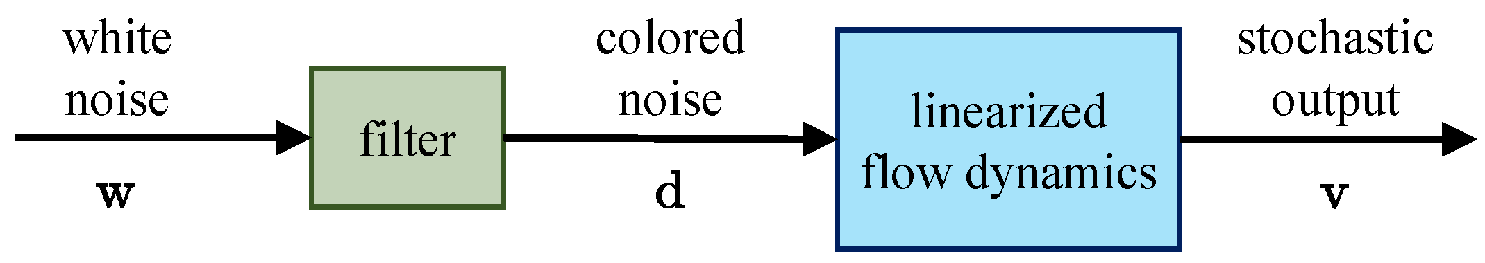
3. Stochastically Forced Linearized Navier–Stokes Equations

In this section, we provide details on the stochastically forced linearized NS equations around a static 2D base flow profile $\overline{\mathbf{u}}$ resulting from a low-fidelity engineering wake model. Our focus is on 2D models of wind farm turbulence that are constrained to horizontal planes at the hub height of wind turbines. We note, however, that the proposed framework is readily generalizable to 3D wind farm models that account for the wall-normal dimension.

The dynamics of small velocity and pressure fluctuations $(\mathbf{v},p)$ around the base flow profile $(\overline{\mathbf{u}},\overline{P})$ are governed by the linearized NS and continuity equations

$$\begin{array}{ccc}\hfill {\mathbf{v}}_t& =& -\left(\mathbf{v}·\nabla \right)\overline{\mathbf{u}}-\left(\overline{\mathbf{u}}·\nabla \right)\mathbf{v}-\nabla p+{\displaystyle \frac{1}{Re}}\mathrm{\Delta }\mathbf{v}-K^{-1}\mathbf{v}+\mathbf{d}\hfill \\ \hfill 0& =& \nabla ·\mathbf{v},\hfill \end{array}$$

(3)

where the momentum equations are augmented with a volume penalization term $K^{-1}\mathbf{v}$ and a zero-mean stationary stochastic $\mathbf{d}$ to capture the effect of turbine structures and trigger a statistical response from the linearized dynamics, respectively. The velocity fluctuations vector consists of streamwise u and spanwise w components of velocity, i.e., $\mathbf{v}={\left[uw\right]}^T$, ∇ is the gradient operator, $\mathrm{\Delta }=\nabla ·\nabla$ is the Laplacian operator, and the Reynolds number $Re=U_{\infty }{d}_0/\nu$ is defined in terms of the rotor diameter $d_0$, the free-stream velocity $U_{\infty }$, and the kinematic viscosity $\nu$. All variables and parameters are non-dimensionalized: length by $d_0$, velocity by $U_{\infty }$, time by $d_0/U_{\infty }$, and pressure by $\rho U_{\infty }^2$.

The volume penalization method adopted in the dynamics of velocity fluctuations (3) avoids the implementation of boundary conditions in complex geometries by modeling the effect of solid obstructions of the flow as a spatially varying permeability function K that influences the governing equations as an additive body force. Within the fluid, the penalization resulting from the permeability function K should have no influence on the flow, i.e., $K\to \infty$, yielding back the original linearized NS dynamics for $\mathbf{v}$. On the other hand, within solid structures, the function K should force the velocity field to zero, i.e., $K\to 0$; see [85] for details. To capture the spatial region that is influenced by the presence of the turbines, we use a smooth 2D filter function of the form

$$K^{-1}(x,z)={\displaystyle \frac{c}{{\pi }^2}}\left[arctan\left(a(x-x_1)\right)-arctan\left(a(x-x_2)\right)\right]\left[arctan\left(a(z-z_1)\right)-arctan\left(a(z-z_2)\right)\right],$$

(4)

where $x_{1,2}$ and $z_{1,2}$ determine the spatial extent of the rotors in the horizontal directions, and parameters a and c determine the slope and magnitude of the function, respectively; see Figure 1 for samples of one-dimensional (1D) and 2D resistance functions $K^{-1}$. Typically, the slope a is set to a reasonably large value that clearly captures the spatial extent of the turbines but does not violate the differentiability of the linearized operator or cause large derivatives of $K^{-1}$. Ideally, the magnitude c would be set to extremely large values to ensure a significant drop in the velocity field within the turbine structures. However, in practice, large values of c can violate the stability of the linearized NS operator. Our numerical experiments suggest that the largest value of c before the linearized dynamics becomes marginally stable (eigenvalues of A in Equation (2) fall on the imaginary axis) provides the best balance in capturing the effect of turbines on the turbulent velocity field while maintaining a well-behaved stable dynamic generator. Figure 1 shows 1D and 2D examples of resistance functions $K^{-1}$ over single- and multi-turbine domains, respectively. When accounting for the presence of yawed turbines, the coordinates and spatial limits $x_{1,2}$ and $z_{1,2}$ in Equation (4) are rotated by the yaw angle; see Figure 2 for an illustration.

In Equation (3), a standard conversion can be used to eliminate pressure and convert the dynamics from a descriptor form to an evolution form. Furthermore, a finite-difference scheme with $N_x$ and $N_z$ discretization points in the streamwise x and spanwise z directions, respectively, may be used to approximate the underlying differential operators and obtain the finite-dimensional state-space representation

$${\dot{\mathbf{v}}}_{(}t)=A\mathbf{v}\left(t\right)+B\mathbf{d}\left(t\right).$$

(5)

with $\mathbf{v}\left(t\right)\in {\mathbb{R}}^{2\times N_x\times N_z}$ and $\mathbf{d}\left(t\right)\in {\mathbb{R}}^{2\times N_x\times N_z}$. See Appendix A for the system matrices, details on the finite-dimensional approximation, and boundary conditions. For the wind farm flow under steady atmospheric conditions, the operator A in Equation (5) has no exponentially growing eigenmodes (i.e., the dynamic matrix A is stable). Thus, subject to zero-mean white-in-time forcing $\mathbf{d}$ with spatial covariance $\mathrm{\Omega }⪰0$, i.e., $\mathbf{E}\left(\mathbf{d}\left(t\right)\right)=0$ and $\mathbf{E}\left(\mathbf{d}\left(t\right){\mathbf{d}}^T\left(\tau \right)\right)=\mathrm{\Omega }\delta (t-\tau )$, the steady-state covariance of the fluctuating velocity field

$$X:=\underset{t\to \infty }{lim}\mathbf{E}\left(\mathbf{v}\left(t\right){\mathbf{v}}^T\left(t\right)\right)$$

can be obtained from the solution to the Lyapunov equation

$$AX+X{A}^T=-B\mathrm{\Omega }{B}^T.$$

(6)

This equation relates the statistics of white-in-time forcing, represented by $\mathrm{\Omega }$, to the infinite-horizon state covariance X via system matrices A and B.

The energy spectrum of the streamwise and spanwise velocity components can be extracted from the diagonal entries of the matrix X, and the total kinetic energy of the flow can be computed as

$$E=\mathrm{trace}\left(X\right)$$

(7)

While white-in-time forcing is useful in studying the receptivity of the turbulent flow to exogenous disturbances [72,73], it is often found to be insufficient in reproducing its statistical signatures [66,67]. To address this issue, we next consider the more general case of colored-in-time stochastic forcing, and pose inverse problems that identify both the statistics of colored-in-time forcing and an input matrix B to match the available second-order statistics of wind farm turbulence using the LTI model (5).

4. Stochastic Dynamical Modeling of Partially Available Second-Order Statistics

Modern-day wind farms use a host of sensing devices that are distributed across the farm to provide critical SCADA data for assessing the performance of the power plant and making changes to the operational settings of wind turbines in real time. The incoming stream of flow measurements from nacelle-mounted anemometers, weather towers, pressure sensors, or even Doppler LiDAR systems can be processed to determine the power extracted by turbines, loads exerted on rotor structures, and the direction and speed of the incoming wind. Time-averaged quantities can also be used to develop wake models that may in turn enable model-based flow estimation and wind farm control synthesis. Moreover, due to advances in high-performance parallel computing, large datasets are becoming accessible from the LES of wind farm flows under various atmospheric conditions. Herein, we utilize such data to realize stochastic forcing models for the linearized NS Equation (5) that yield output velocity statistics that best reproduce the results of LES. We consider the availability of velocity variances at prespecified locations across the wind farm, i.e., second-order statistics of the fluctuating velocity field $\overline{{\mathbf{v}}^2}$, which constitute entries of the covariance matrix X of the linearized model (5). In Section 5.3, we demonstrate how knowledge of a subset of such statistics can suffice in completing the second-order statistical signature of wind farm turbulence. In the remainder of this section, we provide background material regarding the structural constraints on the state covariance matrix X, draw from the stochastic dynamical modeling framework of Zare et al. [66,67,77] to formulate covariance completion problems that identify the statistics of stochastic forcing $\mathbf{d}$ into the linear Gaussian model (5) to reproduce available second-order statistics ${\mathbf{v}}^2$, and provide filter parameterization for the realization of the identified forcing $\mathbf{d}$.

4.1. Second-Order Statistics of LTI Systems

For system (5) with Hurwitz A and controllable pair $(A,B)$, a matrix X qualifies as the steady-state covariance matrix of the state vector, i.e.,

$$X:=\underset{t\to \infty }{lim}\mathbf{E}\left(\mathbf{v}\left(t\right){\mathbf{v}}^T\left(t\right)\right)$$

if and only if the Lyapunov-like equation

$$AX+X{A}^T=-B{H}^T-H{B}^T$$

(8)

is solvable for the matrix H [86,87]. The matrix H quantifies the cross correlation between the input and the state in model (5) [Appendix B] [66]:

$${\displaystyle H:=\underset{t\to \infty }{lim}\mathbf{E}\left[\mathbf{v}\left(t\right){\mathbf{d}}^T\left(t\right)\right]+{\displaystyle \frac{1}{2}}B\mathrm{\Omega }.}$$

When the stochastic input $\mathbf{d}$ is a zero mean and white in time (state-independent) with covariance $\mathrm{\Omega }$, $H=(1/2)B\mathrm{\Omega }$ reduces Equation (8) to the standard algebraic Lyapunov Equation (6). In contrast to the Lyapunov Equation (6), the right-hand side of Equation (8) is generally sign indefinite, i.e., it will have both positive and negative eigenvalues, unless the stochastic forcing $\mathbf{d}$ is white in time. The one-point velocity correlations along the diagonal of the state covariance matrix X constitute velocity variances that are matched in accordance with field measurements across the farm.

4.2. Covariance Completion

Given partially known diagonal entries of X corresponding to velocity variances across the farm, we seek an input matrix B and statistics of forcing $\mathbf{d}$ that are consistent with the hypothesis that the required statistics in $\mathbf{v}$ are generated by model (5) with known generator A. It is also important to restrict the complexity of the identified forcing model, which is quantified as the number of degrees of freedom that are directly influenced by the stochastic forcing, i.e., the number of input channels in matrix B or $rank\left(B\right)$. To these ends, we solve the structured covariance completion problem:

$$\begin{array}{cc}\underset{X,Z}{minimize}& -log\; det\left(X\right)+\mu {\parallel Z\parallel }_{*}\hfill \\ \mathrm{subject} \mathrm{to}& AX+X{A}^T+Z=0\hfill \\ & X\circ E-G=0\hfill \end{array}$$

(9)

which penalizes a composite objective subject to two linear constraints. The first constraint denotes the Lyapunov-like Equation (8) with $Z:=B{H}^T+H{B}^T$, and the second denotes the necessity to match known velocity statistics. Here, the matrices A, E, and G are problem data, and the Hermitian matrices X and Z are optimization variables. Entries of G represent partially available second-order statistics of the velocity field $\mathbf{v}$, the symbol ∘ denotes element-wise matrix multiplication, and E is the structural identity matrix:

$$E_{ij}=\left\{\begin{array}{cc}1,\hfill & \mathrm{if}{G}_{ij}\mathrm{is}\mathrm{available}\hfill \\ 0,\hfill & \mathrm{if}{G}_{ij}\mathrm{is}\mathrm{unavailable}.\hfill \end{array}\right.$$

The objective function provides a trade-off between the solution to a maximum-entropy problem and the complexity of the forcing model; the logarithmic barrier ensures the positive definiteness of the matrix X, and the nuclear norm regularizer, which is weighted by the parameter $\mu >0$, is used as a proxy for the rank function (see, for example, References [88,89]). The rank of the matrix Z bounds the number of independent input channels or columns in matrix B; for details, see [77]. We note that unless the forcing $\mathbf{d}$ in Equation (5) is white in time, the matrix Z may have both positive and negative eigenvalues. Optimization problem (9) is convex and therefore has a globally optimal minimizer because its objective function is convex (linear combination of a strongly convex logarithmic barrier function and a convex regularization term) and its constraint set is linear. Moreover, it can be cast as a semidefinite program and solved efficiently using standard solvers [90,91,92] for small- and medium-size problems. In [77,93,94], customized algorithms were developed to deal with larger problems such as those arising in the modeling of multi-turbine wind farms.

4.3. Stochastic Realization

Problem (9) combines the nuclear norm with an entropy function in order to target low-complexity structures for stochastic forcing and facilitate the construction of a particular class of low-pass filters that generate suitable forcing into Equation (5). Following the spectral factorization technique described in [Section III.B] [77], the solution Z to optimization problem (9), which represents the right-hand side of the Lyapunov-like Equation (8) (i.e., $Z=B{H}^T+H{B}^T$), can be decomposed into matrices B and H. As shown in [Proposition 2] [77], the number of columns in the resulting input matrix B, which also dictates the number of colored-in-time inputs $\mathbf{d}$ in model (5), is given by the maximum of positive and negative eigenvalues of matrix Z. Factors B and H, together with matrix X, which also results from solving problem (9), and the state matrix A, enable the construction of generically minimal linear filters that have the same number of degrees of freedom as system (5). The state-space representation for such filters is given by

$$\begin{array}{ccc}\hfill \dot{\xi }\left(t\right)& =& (A-B{C}_f)\xi \left(t\right)+B\mathbf{w}\left(t\right)\hfill \\ \hfill \mathbf{d}\left(t\right)& =& -C_f\xi \left(t\right)+\mathbf{w}\left(t\right)\hfill \end{array}$$

(10)

where,

$$C_f={\displaystyle \frac{1}{2}}\mathrm{\Omega }{B}^T{X}^{-1}-H^T{X}^{-1}.$$

Here, $\xi$ is the state of the filter, and $\mathbf{w}$ is a zero-mean white-in-time stochastic process with covariance $\mathrm{\Omega }\succ 0$. The state-space representation of the cascade connection of the linear filter (10) and linearized NS dynamics (5) (Figure 3) has twice as many states as the finite-dimensional approximation to linearized dynamics and is not controllable, i.e., it is not minimal. By removing the uncontrollable states, we arrive at a parsimonious (low rank) modification to the original linearized dynamics (see Section II.B of [77] for details):

$$\dot{\mathbf{v}}\left(t\right)=\left(A-B{C}_f\right)\mathbf{v}\left(t\right)+B\mathbf{w}\left(t\right).$$

(11)

The resulting stochastic wake model is linear and maintains a close relation with the physics retained by the linearized NS equations due to the low-rank nature of the modification term $BK$, which follows the column rank deficiency in matrix B. Thus, it is not only convenient for the purpose of conducting linear stochastic simulations and real-time model-based feedback control with provable performance guarantees but it holds the promise of ensuring satisfactory performance, even when the real physical system deviates from the model used for design.

5. Numerical Experiment

In this section, we demonstrate the utility of the stochastic dynamical modeling framework in completing the partially available statistical signature of the turbulent velocity field at the hub height of a wind farm. We begin with a brief discussion into the details of LES, which were used to generate data for the training and verification/validation of our stochastic dynamical models. We also provide details on the analytical base flow model around which we linearize the NS equations. We then focus on a single turbine configuration to assess the value of providing velocity statistics at various distances downstream of the turbine in training our data-enhanced stochastic wake model. Building on the results obtained from this case study, we model the turbulent flow impinging on a $4\times 1$ cascade of turbines. Finally, we provide a dynamical realization for the identified stochastic forcing that drives the linear dynamics of the flow over the turbine cascade and use linear stochastic simulations to validate the output of the overall model.

5.1. Large-Eddy Simulations

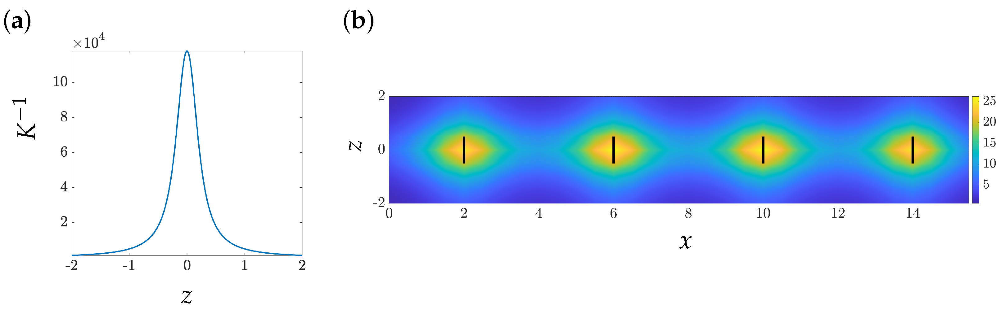
A cascade of four NREL-5MW reference turbines [95] is simulated using the LES code UTD-WF [96,97,98,99], which employs the rotating ADM and the immersed boundary method of Orlandi and Leonardi [100] to respectively account for the effect of the rotating turbine blades and the turbines’ towers and nacelles. The computational box extends $32d_0$, $10.24d_0$ and $10d_0$ in the streamwise, spanwise, and vertical directions, respectively, where $d_0$ is the rotor diameter. The distance between the inlet and the most upstream turbine is equal to $9d_0$. The LES was performed in a computational box with no-slip conditions at the bottom boundary in addition to the surfaces of nacelles and towers, free-slip conditions at the top boundary, periodic boundary conditions in the spanwise direction, and radiative boundary conditions [101] at the outlet. In the vicinity of turbine structures, the grid is uniformly refined in all the three directions with $\mathrm{\Delta }x=\mathrm{\Delta }z=\mathrm{\Delta }y=0.025d_0$, and away from the turbines, the grid is stretched in the vertical direction. Although the resolution is not sufficient to resolve the boundary layer flow around the tower accurately (as in most LES), the impermeability provided by the immersed boundary method reproduces blockage effects and overall momentum loss across the turbine structures.

Neutral atmospheric stability conditions were used in the LES. At the inlet of the computational domain, atmospheric boundary layer conditions were mimicked by superimposing the turbulent velocity field from a precursor simulation to a mean velocity profile expressed by the power law

$$\begin{array}{c}\hfill {\displaystyle \frac{U}{U_{\mathrm{hub}}}}={\left({\displaystyle \frac{y}{y_{\mathrm{hub}}}}\right)}^{\alpha }\end{array}$$

(12)

where U is the streamwise velocity component at height y, $U_{\mathrm{hub}}=U_{\infty }$ is the mean streamwise component of the wind velocity at hub height $y_{\mathrm{hub}}$, and $\alpha$ is the shear exponent, which we set to $0.05$. The upstream velocity $U_{\infty }$ is chosen to be about $0.8U_{\mathrm{rated}}$, where the rated wind speed $U_{\mathrm{rated}}$ is set to $11.4$ m/s [95]. This allows using a standard region II control law [102,103] for the rotor dynamics, where each turbine is assumed to extract the maximal energy from the incoming flow. The superposition of the mean flow in Equation (12) and the turbulence from the precursor simulation ultimately results in a hub-height turbulence intensity of $8\%$ impinging the first turbine in the cascade. The precursor simulation was performed in a computational box with periodic boundary conditions in both streamwise and spanwise directions, with no-slip conditions at the bottom and free-slip conditions at the top. To promote the generation of turbulence, roughness cubes with a height of $0.1y_h$ were placed at the bottom of the computational box in a manner that ensures the recovery of the log-law profile before the sampling plane for the wind farm simulation [104].

The time-averaged and root mean square profiles of velocity fluctuations are computed using 750 instantaneous snapshots of the 3D velocity field generated by LES. These snapshot were taken over a period of about 27 min of real-time operation (150 non-dimensional time units based on a reference length and speed of 126 m and $11.4$ m/s) with a temporal resolution of about 2 s ($0.2$ non-dimensional time units). In accordance with the LES, the numerical experiments herein consider $Re=8\times {10}^7$ based on $d_0$ and $U_{\infty }$.

5.2. Base Flow

Our stochastic models are based on the stochastically forced linearized NS equations around a static base flow profile $\overline{\mathbf{u}}$ with an analytical expression provided by a low-fidelity engineering wake model. For simplicity, we restrict the computational domain to the 2D space at hub height, and assume zero cross wind, which means that the base flow will only contain one non-zero component in the streamwise direction. We use the wake model proposed in reference [105], which accounts for the deflection in the wake trajectory resulting from the misalignment of the turbine rotor against the wind direction. We note, however, that our framework allows for the incorporation of more complex wake models that may result in improved predictions of the velocity fluctuation field. Herein, we summarize the equations that describe the streamwise velocity profile provided by Bastankhah and Porté-Agel [105] in addition to the values of parameters used in generating the results in the following subsections. This wake velocity field is given by [105]

$$U(x,z)=U_{\infty }-U_{\infty }\left(1-\sqrt{1-{\displaystyle \frac{C_{T}cos\left(\gamma \right)}{8\left({\sigma }_y{\sigma }_z\right)}}}\right){\mathrm{e}}^{-{\displaystyle \frac{1}{2}}\left[{\left({\displaystyle \frac{y-y_h}{{\sigma }_y}}\right)}^2+{\left({\displaystyle \frac{z-\delta }{{\sigma }_z}}\right)}^2\right]}$$

(13)

where all length scales are non-dimensionalized by the rotor diameter $d_0$, $\gamma$ is the yaw angle, $y_h$ is the hub height, $C_T$ is the thrust coefficient, $\delta$ is the spanwise deflection of the wake centerline, and wake parameters ${\sigma }_y$ and ${\sigma }_z$ are given by

$${\sigma }_y=k\left(x-x_0\right)+{\displaystyle \frac{1}{\sqrt{8}}};{\sigma }_z=k\left(x-x_0\right)+{\displaystyle \frac{cos\left(\gamma \right)}{\sqrt{8}}}$$

(14)

where k is the wake growth rate, and $x_0$ is the potential core length computed as

$$x_0={\displaystyle \frac{cos\left(\gamma \right)\left(1+\sqrt{1-C_T}\right)}{\sqrt{2}\left(4\alpha \mathit{I}+{\beta }^{★}\left(1-\sqrt{1-C_T}\right)\right)}}.$$

The potential core length $x_0$ is used to demarcate the near- ($x\le x_0$) and far-wake ($x>x_0$) regions. In the near-wake region, $\delta ={\theta }_{c0}x$, and in the far-wake region,

$$\delta ={\theta }_{c0}{x}_0+{\displaystyle \frac{{\theta }_{c0}}{14.7}}\sqrt{{\displaystyle \frac{cos\left(\gamma \right)}{k{C}_T}}}\left(2.9+1.3\sqrt{1-C_T}-C_T\right)ln\left[{\displaystyle \frac{(1.6+\sqrt{C_T})\left(1.6\sqrt{{\displaystyle \frac{8{\sigma }_y{\sigma }_z}{cos\left(\gamma \right)}}}-\sqrt{C_T}\right)}{(1.6-\sqrt{C_T})\left(1.6\sqrt{{\displaystyle \frac{8{\sigma }_y{\sigma }_z}{cos\left(\gamma \right)}}}+\sqrt{C_T}\right)}}\right]$$

where ${\theta }_{c0}$ is the deflection angle between the wake and the free-stream flow in the near-wake region and is given by ${\theta }_{c0}=0.3\gamma \left(1-\sqrt{1-C_{T}cos\left(\gamma \right)}\right)/cos\left(\gamma \right)$. Figure 4a provides an illustration of the geometric parameters that characterize this Gaussian wake model. Finally, when considering multi-turbine farms, we follow a linear superposition law to capture velocity deficits in the overlapping regions where wakes interact [41,106]. Based on this, the velocity at any given spatial location $(x,z)$ within a multi-turbine wind farm is given by

$$U(x,z)=U_{\infty }-\sum _k\left(U_{\infty }-U_k(x,z)\right)$$

where $U_k$ denotes the wake velocity of the k-th turbine computed using Equation (13). Our numerical experiments (not presented for brevity) show little gain when using more sophisticated (e.g., root-sum-squared) superposition laws [29,107].

In generating the results presented in the remainder of this section, the horizontal dimensions are uniformly discretized with ${\mathrm{\Delta }}_x={\mathrm{\Delta }}_z=0.125$. Furthermore, in Equation (14) the choice of $k=0.022$ follows Ref. [105] and $C_T=0.787$ is associated with the peak power production of a 5 MW NREL turbine [95] using an LES code that incorporates blade momentum element theory [97,108]. We note that the choice of base velocity parameters could be guided by the origin of the flow statistics used in training the stochastic model of flow fluctuations (cf. Section 4.2), e.g., LES in this paper. In other words, if instead of LES data, the training dataset consisted of velocity correlations measured via a field campaign, the wake growth rate k in Equation (14), which itself depends on the turbulence intensity, could be chosen in a consistent manner with the experimental measurements. Figure 4b shows the static 2D velocity field predicted by Equation (13) for a 4-turbine cascade configuration with equal spacing and yaw.

5.3. Predicting Second-Order Turbulence Statistics

In this section, we evaluate the predictive capability of our stochastic modeling framework in completing the statistical signature of the hub-height turbulent velocity field in single-turbine and four-turbine cascade configurations. Specifically, we assume knowledge of the streamwise and spanwise velocity variances at various diameters behind wind turbines and predict the remainder of the second-order statistical signature of the flow using the stochastically forced linearized NS model (5). The available turbulence statistics may be provided by field measurement devices such as LiDAR systems that are deployed in wind farms to scan and monitor hub-height wind [109]. Herein, the turbulence statistics that are made available to the optimization framework are computed from time-resolved LES-generated velocity fields. For consistency with precursor simulations that have been used to generate turbulent inflow conditions for the LES, all numerical experiments assume knowledge of velocity statistics at all data points upwind of the leading turbine. The optimization framework of Section 4.2 identifies the appropriate colored-in-time forcing to the linearized NS equations to account for the available statistics and predict unavailable ones by virtue of the physics-based nature of model (5).

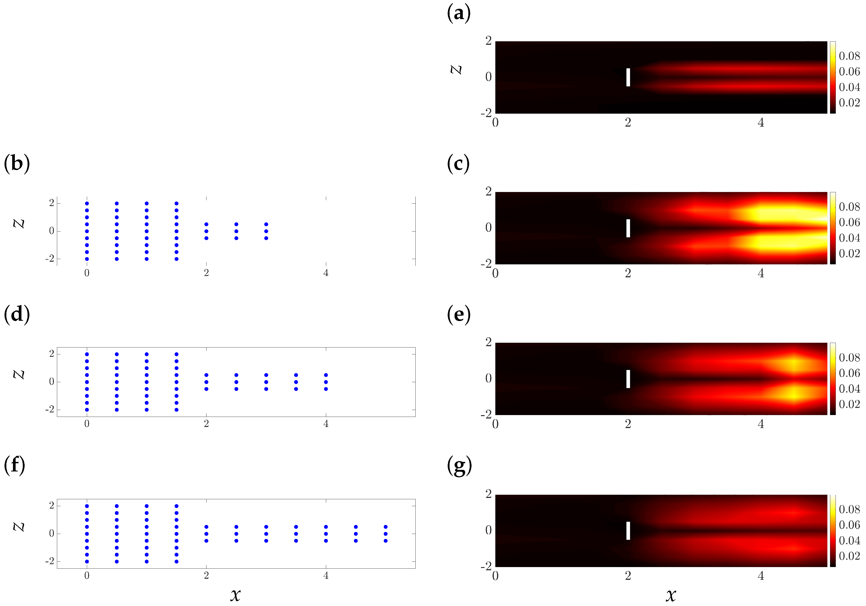
5.3.1. Predicting the Wake of a Single Turbine Using Partially Available Flow Statistics

We first focus on the problem of predicting the streamwise and spanwise velocity variances ($uu$ and $ww$) at the hub height of a single unit-diameter wind turbine located at $x=2$ and $z=0$ in a 2D computational domain of size $L_x\times L_z=5\times 4$ with $x\in [0,5]$ and $z\in [-2,2]$. We use $N_x=13$ and $N_z=9$ equally spaced collocation points to discretize the computational domain in the streamwise x and spanwise z directions, respectively, thereby rendering the state in model (5) $\mathbf{v}={\left[uw\right]}^T\in {\mathbb{R}}^{234\times 1}$. The base flow around which we linearize the NS equations is generated using the analytical expression in Equation (13) (Figure 5b). We consider three cases in which the available training dataset contains three streams of streamwise and spanwise velocity variance measurements from behind the blade tips (edges of 2D rotor structure) and the turbine nacelle (middle of rotor structure) and at various distances away from the turbine: (i) at the turbine location $x=2$ and points within one diameter away (Figure 6c and Figure 7c), (ii) at $x=2$ and points within two diameters away (Figure 6e and Figure 7e), and (iii) at $x=2$ and points within three diameters away (Figure 6g and Figure 7g). As is evident in Figure 6g and Figure 7g, for the considered turbine and atmospheric conditions, access to flow statistics three diameters away from the turbine can significantly improve the completion of the statistical signature of the flow at hub height. Our results demonstrate the ability of the data-enhanced linearized NS equations to capture the dominant trends of $uu$ and $ww$ in the wake of a turbine.

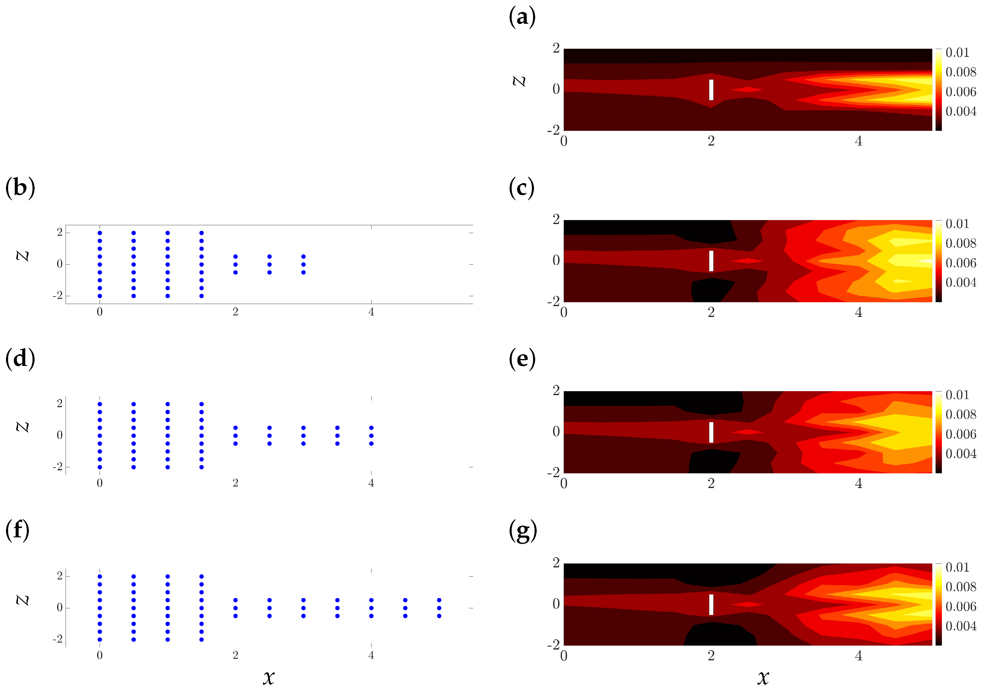
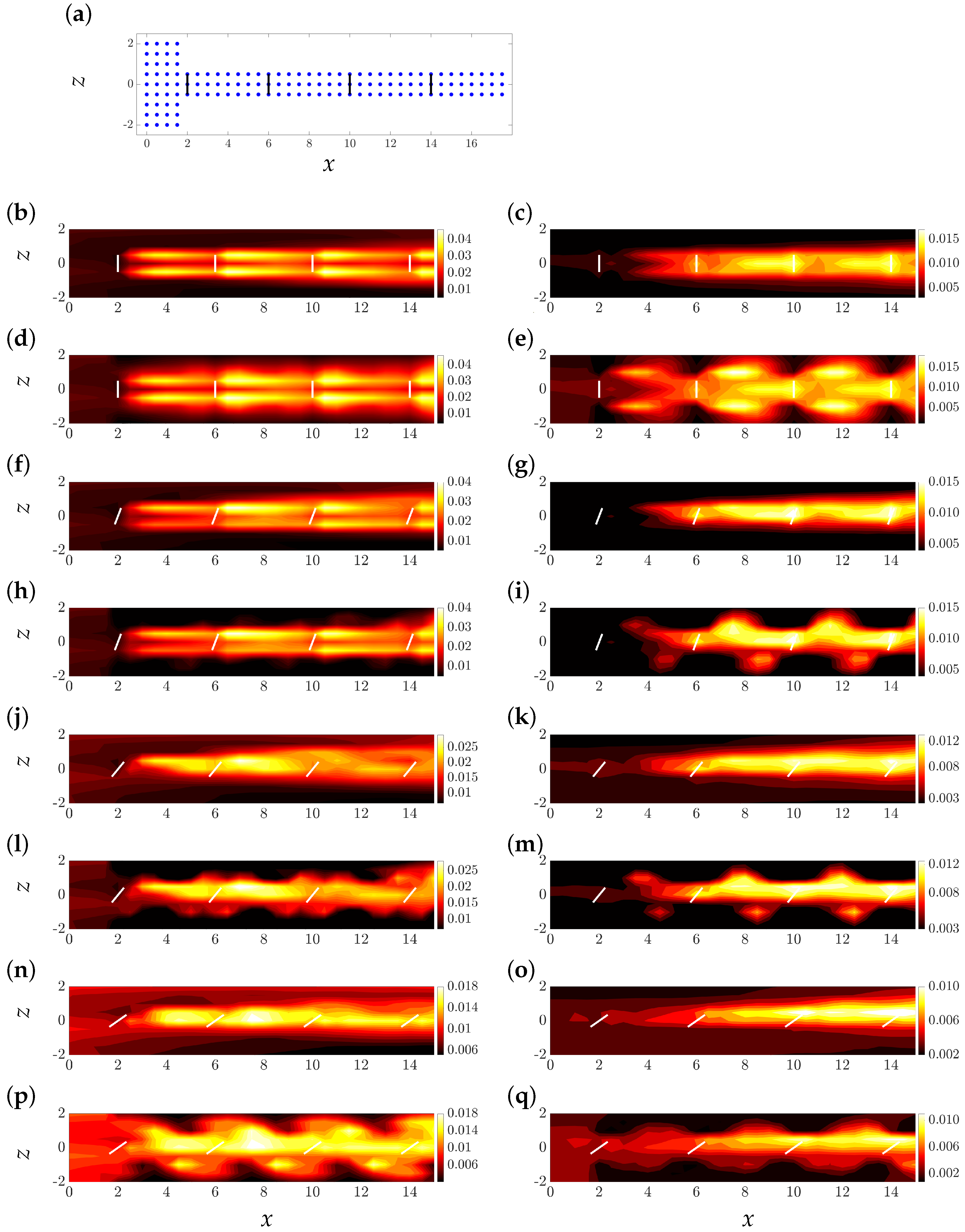
5.3.2. Predicting Wind Farm Turbulence Impinging on a Cascade of Turbines

We further extend our study to the case of a $4\times 1$ array of uniformly yawed wind turbines of a unit diameter. For this experiment, we consider a 2D computational domain at hub height with $x\in [0,16]$ and $z\in [-2,2]$. The turbines are located at $x=\{2,6,10,14\}$ and $z=0$. We use a similarly spaced grid as the single-turbine experiment in the previous subsection with $N_x=38$ and $N_z=9$ equally spaced collocation points that render the state in model (5) $\mathbf{v}={\left[uw\right]}^T\in {\mathbb{R}}^{684\times 1}$. Given the findings of the previous subsection, for the best recovery of velocity variances, we use LES-generated statistics within three diameters behind the tips and nacelle of each of the turbines as training data for our stochastic models of the hub-height velocity field (Figure 8a). We note that the same data points are used by the optimization framework, even for the cases where the turbines are yawed.

Figure 8 compares the streamwise and spanwise velocity variances $uu$ and $ww$ predicted by our data-enhanced physics-based model with the results of LES. As evident from the energetic patches throughout the farm, our model over-predicts the overall energy of the flow while capturing dominant qualitative features of the streamwise velocity correlations, such as the distribution of high and low energy over the domain and the spanwise asymmetry due to the turbines’ rotation. The latter features are especially well captured for yaw angles up to ${30}^{\circ }$. We note that for the full-wake scenarios (i.e., when downwind turbines are entirely in the wake of upwind ones), the velocity variances look similar to the double-peak pattern modeled from analytical models offered by Ref. [38]. Our model also captures the coalescence of high-turbulence streams behind the first two turbines’ blade tips for lower yaw angles. The quality of completion for the second-order statistical signature of the turbulent flow depreciates for the largest yaw angle ($\gamma ={45}^{\circ }$), as spurious regions of high energy appear below the actual wake zone (Figure 8p). Uncovering the potential reasons behind such irregular predictions calls for additional in-depth examination. We note, however, that such extreme misalignment is not conducive to reasonable levels of power generation [110].

The right column in Figure 8 presents the spanwise velocity variance $ww$ for different yaw angles resulting from our model and LES. In contrast to the predictions of the streamwise variance $uu$, we see that the quality of predictions of $ww$ improve as the yaw angle increases. This is especially evident for $\gamma ={30}^{\circ }$ (Figure 8m) and ${45}^{\circ }$ (Figure 8q). Our model does well in capturing the high-energy regions within the turbine wakes, although spurious regions of high energy are created just outside the wake zones. Uncovering potential reasons behind such irregular predictions in the spanwise variance calls for additional in-depth examination.

Our linear stochastic dynamical models enable a good quality of statistical completion and replicate the dominant features of the flow (shown in Figure 8), even for the larger yaw angles where the deflected wake zone lies far beyond many of the training data points. The intrinsic physics-based nature of the model combined with the Lyapunov-like constraint in the covariance completion problem (9) [66,67] allows the model to stay authentic to the flow physics (as captured by the linearized dynamics) while imposing consistency between the data and the linearized NS dynamics.

In optimization problem (9), the regularization parameter $\mu$ determines the importance of the nuclear norm of matrix Z relative to the logarithmic barrier function of the covariance matrix X. Larger values of $\mu$ yield lower-rank matrices Z but may compromise the quality of completion; see Appendix C of [66]. In this study, $\mu =100$ was observed to provide the best quality of reproduction of the turbulence statistics for both single- and multi-turbine configurations. In training the stochastic model for the $4\times 1$ cascade of turbines at $\gamma =0^{\circ }$ yaw (Figure 8d,e), where $N_x=38$ and $N_z=9$ (Z is a square matrix of size 684), the choice of $\mu =100$ in problem (9) results in a Z matrix with 1 negative and 265 positive eigenvalues ($rank\left(Z\right)=266$). As discussed in Section 4.1, the presence of both positive and negative eigenvalues in matrix Z indicates that the second-order statistics of wind farm turbulence cannot be reproduced by the linearized NS equations with white-in-time stochastic excitation. The distribution of eigenvalues of matrix Z also indicates that 265 colored-in-time inputs are required to reproduce the partially available entries in covariance matrix X corresponding to the known velocity variances (cf. Figure 3); see [66,77] for additional details.

5.4. Verification in Stochastic Linear Simulations

As discussed in the prior subsection, the matrix Z that results from solving the covariance completion problem (9) for the $4\times 1$ cascade of turbines at $\gamma =0^{\circ }$ yaw with a choice of $\mu =100$ has 1 negative and 265 positive eigenvalues. Following the discussion in Section 4.3, matrix Z can be decomposed into $B{H}^T+H{B}^T$, with the input matrix B having 265 independent columns. In other words, the identified matrix X from solving problem (9) can be explained by driving the LTI model (5) with 265 stochastic inputs $\mathbf{d}$. The solution to the covariance completion problem (9) also determines the dynamics of the linear filter (10) that generates the colored-in-time forcing $\mathbf{d}$ with appropriate power spectral density.

We conduct stochastic linear simulations to verify our stochastic model of wind farm turbulence (Equation (5)). Since a proper comparison with LES requires ensemble averaging, rather than comparison at the level of individual stochastic simulations, we conducted 20 simulations of system (5)). The total simulation time was set to 300 time units. Figure 9 shows the time evolution of the energy (variance) of velocity fluctuations ${\mathbf{v}}^T\left(t\right)\mathbf{v}\left(t\right)$ for 20 realizations of white-in-time forcing of the filter dynamics, generating the colored-in-time input $\mathbf{d}$ and exciting the linear dynamical model (5). The variance averaged over all simulations is marked by the thick black line, which asymptotically approaches the value of the total turbulent kinetic energy (averaged over space) in the statistical steady state $\mathrm{trace}\left(X\right)$ (Equation (7)). The ensemble average of the velocity fields generated by the 20 simulations of Equation (5) result in second-order statistics that have $4.1\%$ relative error in matching the training data provided by LES. This close agreement can be further improved by running additional linear simulations and by increasing the total simulation times.

6. Concluding Remarks

We provide a framework for the stochastic dynamical modeling of wind farm flow fluctuations that is based on the stochastically forced linearized NS equations. To obtain the dynamics of velocity fluctuations, we choose to linearize the NS equations around the the Gaussian engineering wake model, which is capable of capturing the long-time attributes of the waked velocity field behind yawed wind turbines. We force the linearized dynamics with stochastic input to trigger a stochastic response that may capture the statistical characteristics of wake turbulence. In lieu of a turbulence model, however, we follow the inverse modeling approach of [66,67,77] and shape the spectral content of the input forcing via convex optimization so that the output of the linearized dynamics matches the statistical signatures of the turbulent wake. To this end, we use a partial set of velocity correlations computed from an experimentally or numerically generated dataset. In this paper, we focus on the development of a 2D model of the hub-height velocity field and use LES-based velocity correlations, namely the normal and shear stress profiles from prespecified locations across a wind farm, to realize colored-in-time stochastic forcing that mimics the effect of background turbulence for our linearized NS dynamics. We demonstrate the efficacy of our models in not only reproducing available correlations of the turbulent velocity field over multi-turbine wind farms but also reasonably completing the statistical signature of the flow wherever correlations were not available in accordance with LES. This also allows us to examine the value of velocity correlations from various distances behind wind turbine rotors in completing the statistical signature of hub-height turbulence and capturing regions of high and low turbulence.

6.1. Discussion

Our approach uses data from field measurements or high-fidelity numerical simulations to enhance the predictive capability of a physics-based model resulting from linearization of the NS equations around an analytical base flow profile. In addition to ensuring statistical consistency, the convex optimization problem used in identifying the source of stochastic excitation restricts the number of degrees of freedom in the linearized model that are directly influenced by the colored-in-time forcing (cf. Section 4.2). This feature allows us to preserve the relevance of the linearized NS equations as a physics-based model that can overcome potential robustness issues of solely data-driven models in capturing the high variability of atmospheric turbulence. As shown in Section 5.3.2, this allows us to maintain good levels of statistical recovery from fixed data-collections points, even when yaw misalignment relative to the incoming wind direction causes turbine wakes to deflect away from the centerline. In other words, maintaining the locations of the training data from the non-yawed case does not compromise model predictions when turbine rotors are yawed. Moreover, the yaw-based parameterization of our base flow model (Equation (13)) allows for online parametric updates in accordance with varying atmospheric conditions that may be informed by, for example, SCADA measurements.

The characteristic features of our models that render them desirable for estimation and control are their (i) physics-based dynamic nature, (ii) linearity, (iii) low computational complexity, and (iv) statistical consistency in matching flow quantities that are of interest in flow analysis and control. As they capture the dynamics of small velocity fluctuations, the utility of our models lies in capturing small wind variations that are pertinent to turbine control in below-rated wind speeds (regions 2 and 2.5), e.g., in mitigating mechanical loads. Finally, the inexpensive stochastic linear simulations of Section 5.4, which we use to verify our stochastic dynamical models, highlight the ease in using our models for generating statistically consistent turbulent inflow conditions for numerical simulations.

6.2. Future Work

The modeling framework proposed in this paper allows for alternative wind farm layouts or more sophisticated base flow profiles that better represent the effects of turbine yawing such as those involving wake curl and deflection. Our research program is focused on the development of 3D model extensions that resolve the velocity field down to the ground, thereby enabling ground-sensing capabilities in wind farms. Our long-term goals involve the use of linear stochastic dynamical models for real-time wind forecasting via sequential data assimilation, e.g., Kalman filtering, potential extensions that may account for large shifts in the direction and intensity of incoming wind through a discrete set of base states for linearization, and the use of alternative covariance completion formulations [78,79] in place of problem (9). Given the physics-based nature of our models, the latter research direction can prove decisive in identifying critical wind directions and salient dynamical couplings and interactions in turbine wakes, thereby informing data-acquisition campaigns in assessing the value of one- or two-point velocity correlations in statistical modeling. We also anticipate the application of the stochastic dynamical modeling framework used in this paper to uncertainty modeling problems pertaining to energy storage and network planning [111].

References

1. Fleming, P.; Annoni, J.; Shah, J.J.; Wan, L.; Ananthan, S.; Zhang, Z.; Hutchings, K.; Wang, P.; Chen, W.; Chen, L. Field test of wake steering at an offshore wind farm. Wind Energy Sci. 2017, 2, 229–239. [Google Scholar] [CrossRef]
2. Ahmad, T.; Basit, A.; Ahsan, M.; Coupiac, O.; Girard, N.; Kazemtabrizi, B.; Matthews, P.C. Implementation and analyses of yaw based coordinated control of wind farms. Energies 2019, 12, 1266. [Google Scholar] [CrossRef]
3. Duc, T.; Coupiac, O.; Girard, N.; Giebel, G.; Göçmen, T. Local turbulence parameterization improves the Jensen wake model and its implementation for power optimization of an operating wind farm. Wind Energy Sci. 2019, 4, 287–302. [Google Scholar] [CrossRef]
4. Howland, M.F.; Lele, K.S.; Dabiri, J.O. Wind farm power optimization through wake steering. Proc. Natl. Acad. Sci. USA 2019, 116, 14495–14500. [Google Scholar] [CrossRef] [PubMed]
5. Fleming, P.; King, J.; Simley, E.; Roadman, J.; Scholbrock, A.; Murphy, P.; Lundquist, J.K.; Moriarty, P.; Fleming, K.; van Dam, J.; et al. Continued results from a field campaign of wake steering applied at a commercial wind farm–Part 2. Wind Energy Sci. 2020, 5, 945–958. [Google Scholar] [CrossRef]
6. Bossanyi, E.A.; Ruisi, R. Axial induction controller field test at Sedini wind farm. Wind. Energy Sci. Discuss. 2021, 6, 389–408. [Google Scholar] [CrossRef]
7. Doekemeijer, B.M.; Kern, S.; Maturu, S.; Kanev, S.; Salbert, B.; Schreiber, J.; Campagnolo, F.; Bottasso, C.L.; Schuler, S.; Wilts, F.; et al. Field experiment for open-loop yaw-based wake steering at a commercial onshore wind farm in Italy. Wind Energy Sci. 2021, 6, 159–176. [Google Scholar] [CrossRef]
8. Simley, E.; Fleming, P.; Girard, N.; Alloin, L.; Godefroy, E.; Duc, T. Results from a wake-steering experiment at a commercial wind plant: Investigating the wind speed dependence of wake-steering performance. Wind Energy Sci. 2021, 6, 1427–1453. [Google Scholar] [CrossRef]
9. Johnson, K.E.; Fritsch, G. Assessment of extremum seeking control for wind farm energy production. Wind Eng. 2012, 36, 701–715. [Google Scholar] [CrossRef]
10. Creaby, J.; Li, Y.; Seem, J.E. Maximizing wind turbine energy capture using multivariable extremum seeking control. Wind Eng. 2009, 33, 361–387. [Google Scholar] [CrossRef]
11. Ciri, U.; Rotea, M.A.; Leonardi, S. Model-free control of wind farms: A comparative study between individual and coordinated extremum seeking. Renew. Energy 2017, 113, 1033–1045. [Google Scholar] [CrossRef]
12. Ciri, U.; Rotea, M.A.; Santoni, C.; Leonardi, S. Large-eddy simulations with extremum-seeking control for individual wind turbine power optimization. Wind Energy 2017, 20, 1617–1634. [Google Scholar] [CrossRef]
13. Ciri, U.; Leonardi, S.; Rotea, M.A. Evaluation of log-of-power extremum seeking control for wind turbines using large eddy simulations. Wind Energy 2019, 22, 992–1002. [Google Scholar] [CrossRef]
14. Kumar, D.; Rotea, M.A. Wind Turbine Power Maximization Using Log-Power Proportional-Integral Extremum Seeking. Energies 2022, 15, 1004. [Google Scholar] [CrossRef]
15. Zho, K.; Doyle, J.C. Essentials of Robust Control; Prentice Hall: Upper Saddle River, NJ, USA, 1998; Volume 104. [Google Scholar]
16. Skogestad, S.; Postlethwaite, I. Multivariable Feedback Control: Analysis and Design; Wiley: New York, NY, USA, 2007; Volume 2. [Google Scholar]
17. Goit, J.P.; Meyers, J. Optimal control of energy extraction in wind-farm boundary layers. J. Fluid Mech. 2015, 768, 5–50. [Google Scholar] [CrossRef]
18. Goit, J.P.; Munters, W.; Meyers, J. Optimal coordinated control of power extraction in LES of a wind farm with entrance effects. Energies 2016, 9, 29. [Google Scholar] [CrossRef]
19. Munters, W.; Meyers, J. An optimal control framework for dynamic induction control of wind farms and their interaction with the atmospheric boundary layer. Philos. Trans. R. Soc. Math. Phys. Eng. Sci. 2017, 375, 20160100. [Google Scholar] [CrossRef]
20. Munters, W.; Meyers, J. Towards practical dynamic induction control of wind farms: Analysis of optimally controlled wind-farm boundary layers and sinusoidal induction control of first-row turbines. Wind Energy Sci. 2018, 3, 409–425. [Google Scholar] [CrossRef]
21. Munters, W.; Meyers, J. Dynamic strategies for yaw and induction control of wind farms based on large-eddy simulation and optimization. Energies 2018, 11, 177. [Google Scholar] [CrossRef]
22. Bauweraerts, P.; Meyers, J. On the feasibility of using large-eddy simulations for real-time turbulent-flow forecasting in the atmospheric boundary layer. Bound. Layer Meteorol. 2019, 171, 213–235. [Google Scholar] [CrossRef]
23. Doekemeijer, B.M.; van Wingerden, J.W.; Fleming, P.A. A tutorial on the synthesis and validation of a closed-loop wind farm controller using a steady-state surrogate model. In Proceedings of the 2019 American Control Conference (ACC), Philadelphia, PA, USA, 10–12 July 2019; pp. 2825–2836. [Google Scholar]
24. Singh, P.; Seiler, P. Controlling the meandering wake using measurement feedback. In Proceedings of the 2019 American Control Conference (ACC), Philadelphia, PA, USA, 10–12 July 2019; pp. 4144–4150. [Google Scholar]
25. Doekemeijer, B.M.; van der Hoek, D.; van Wingerden, J.W. Closed-loop model-based wind farm control using FLORIS under time-varying inflow conditions. Renew. Energy 2020, 156, 719–730. [Google Scholar] [CrossRef]
26. Meyers, J.; Bottasso, C.; Dykes, K.; Fleming, P.; Gebraad, P.; Giebel, G.; Göçmen, T.; van Wingerden, J.W. Wind farm flow control: Prospects and challenges. Wind Energy Sci. Discuss. 2022, 7, 2271–2306. [Google Scholar] [CrossRef]
27. Sood, I.; Meyers, J. Tuning of an engineering wind farm model using measurements from Large Eddy Simulations. J. Phys. Conf. Ser. 2022, 2265, 022045. [Google Scholar] [CrossRef]
28. Jensen, N.O. A Note on Wind Generator Interaction; Risø National Laboratory: Roskilde, Denmark, 1983. [Google Scholar]
29. Katic, I.; Højstrup, J.; Jensen, N.O. A simple model for cluster efficiency. In Proceedings of the European Wind Energy Association Conference and Exhibition, Rome, Italy, 7–9 October 1986; Volume 1, pp. 407–410. [Google Scholar]
30. Ainslie, J.F. Calculating the flowfield in the wake of wind turbines. J. Wind Eng. Ind. Aerodyn. 1988, 27, 213–224. [Google Scholar] [CrossRef]
31. Burton, T.; Jenkins, N.; Sharpe, D.; Bossanyi, E. Wind Energy Handbook; John Wiley & Sons: Hoboken, NJ, USA, 2011. [Google Scholar]
32. Frandsen, S.; Barthelmie, R.; Pryor, S.; Rathmann, O.; Larsen, S.; Højstrup, J.; Thøgersen, M. Analytical modelling of wind speed deficit in large offshore wind farms. Wind. Energy Int. J. Prog. Appl. Wind. Power Convers. Technol. 2006, 9, 39–53. [Google Scholar] [CrossRef]
33. Bastankhah, M.; Porté-Agel, F. A new analytical model for wind-turbine wakes. Renew. Energy 2014, 70, 116–123. [Google Scholar] [CrossRef]
34. Martínez-Tossas, L.A.; Annoni, J.; Fleming, P.A.; Churchfield, M.J. The aerodynamics of the curled wake: A simplified model in view of flow control. Wind Energy Sci. 2019, 4, 127–138. [Google Scholar] [CrossRef]
35. Martínez-Tossas, L.A.; Branlard, E. The curled wake model: Equivalence of shed vorticity models. J. Phys. Conf. Ser. 2020, 1452, 012069. [Google Scholar] [CrossRef]
36. Zong, H.; Porté-Agel, F. A point vortex transportation model for yawed wind turbine wakes. J. Fluid Mech 2020, 890, A8. [Google Scholar] [CrossRef]
37. Bastankhah, M.; Shapiro, C.R.; Shamsoddin, S.; Gayme, D.F.; Meneveau, C. A vortex sheet based analytical model of the curled wake behind yawed wind turbines. J. Fluid Mech. 2022, 933, A2. [Google Scholar] [CrossRef]
38. Li, L.; Huang, Z.; Ge, M.; Zhang, Q. A novel three-dimensional analytical model of the added streamwise turbulence intensity for wind-turbine wakes. Energy 2022, 238, 121806. [Google Scholar] [CrossRef]
39. Li, L.; Wang, B.; Ge, M.; Huang, Z.; Li, X.; Liu, Y. A novel superposition method for streamwise turbulence intensity of wind-turbine wakes. Energy 2023, 276, 127491. [Google Scholar] [CrossRef]
40. Krogstad, P.Å.; Davidson, P.A. Near-field investigation of turbulence produced by multi-scale grids. Phys. Fluids 2012, 24, 035103. [Google Scholar] [CrossRef]
41. Niayifar, A.; Porté-Agel, F. Analytical Modeling of Wind Farms: A New Approach for Power Prediction. Energies 2016, 9, 741. [Google Scholar] [CrossRef]
42. Larsen, G.C.; Madsen, H.A.; Thomsen, K.; Larsen, T.J. Wake meandering: A pragmatic approach. Wind Energy 2008, 11, 377–395. [Google Scholar] [CrossRef]
43. Annoni, J.; Howard, K.; Seiler, P.; Guala, M. An experimental investigation on the effect of individual turbine control on wind farm dynamics. Wind Energy 2016, 19, 1453–1467. [Google Scholar] [CrossRef]
44. Iungo, G.V.; Viola, F.; Ciri, U.; Leonardi, S.; Rotea, M. Reduced order model for optimization of power production from a wind farm. In Proceedings of the 34th Wind Energy Symposium, Wind Energy Symposium, San Diego, CA, USA, 4–8 January 2016; p. 2200. [Google Scholar]
45. Boersma, S.; Doekemeijer, B.; Vali, M.; Meyers, J.; van Wingerden, J.W. A control-oriented dynamic wind farm model: WFSim. Wind Energy Sci. 2018, 3, 75–95. [Google Scholar] [CrossRef]
46. Letizia, S.; Iungo, G.V. Pseudo-2D RANS: A LiDAR-driven mid-fidelity model for simulations of wind farm flows. J. Renew. Sustain. Energy 2022, 14, 023301. [Google Scholar] [CrossRef]
47. Scott, R.; Martínez-Tossas, L.; Bossuyt, J.; Hamilton, N.; Cal, R.B. Evolution of eddy viscosity in the wake of a wind turbine. Wind Energy Sci. 2023, 8, 449–463. [Google Scholar] [CrossRef]
48. Annoni, J.; Bay, C.; Johnson, K.; Dall’Anese, E.; Quon, E.; Kemper, T.; Fleming, P. Wind direction estimation using SCADA data with consensus-based optimization. Wind Energy Sci. 2019, 4, 355–368. [Google Scholar] [CrossRef]
49. Bernardoni, F.; Ciri, U.; Rotea, M.A.; Leonardi, S. Identification of wind turbine clusters for effective real time yaw control optimization. J. Renew. Sustain. Energy 2021, 13, 043301. [Google Scholar] [CrossRef]
50. Starke, G.M.; Stanfel, P.; Meneveau, C.; Gayme, D.F.; King, J. Network based estimation of wind farm power and velocity data under changing wind direction. In Proceedings of the 2021 American Control Conference, New Orleans, LA, USA, 26–28 May 2021; pp. 1803–1810. [Google Scholar]
51. Zhang, H.; Chen, J.; Tian, T. Bayesian inference of stochastic dynamic models using early-rejection methods based on sequential stochastic simulations. IEEE/ACM Trans. Comput. Biol. Bioinform. 2020, 19, 1484–1494. [Google Scholar] [CrossRef] [PubMed]
52. Liu, Y.; Nair, N.K.C. A two-stage stochastic dynamic economic dispatch model considering wind uncertainty. IEEE Trans. Sustain. Energy 2015, 7, 819–829. [Google Scholar] [CrossRef]
53. VerHulst, C.; Meneveau, C. Large eddy simulation study of the kinetic energy entrainment by energetic turbulent flow structures in large wind farms. Phys. Fluids 2014, 26, 025113. [Google Scholar] [CrossRef]
54. Annoni, J.; Gebraad, P.; Seiler, P. Wind farm flow modeling using an input-output reduced-order model. In Proceedings of the 2016 American Control Conference (ACC), Boston, MA, USA, 6–8 July 2016; pp. 506–512. [Google Scholar]
55. Raach, S.; Schlipf, D.; Cheng, P.W. Lidar-based wake tracking for closed-loop wind farm control. Wind Energy Sci. 2017, 2, 257–267. [Google Scholar] [CrossRef]
56. Sinner, M.; Pao, L.Y.; King, J. Estimation of large-scale wind field characteristics using supervisory control and data acquisition measurements. In Proceedings of the 2020 American Control Conference (ACC), Denver, CO, USA, 1–3 July 2020; pp. 2357–2362. [Google Scholar]
57. Noack, B.R.; Morzyński, M.; Tadmor, G. Reduced-Order Modelling for Flow Control; CISM Courses and Lectures; Springer: Berlin/Heidelberg, Germany, 2011; Volume 528. [Google Scholar]
58. Tadmor, G.; Noack, B.R. Bernoulli, Bode, and Budgie [Ask the Experts]. IEEE Contr. Syst. Mag. 2011, 31, 18–23. [Google Scholar]
59. Wang, J.X.; Wu, J.L.; Xiao, H. Physics-informed machine learning approach for reconstructing Reynolds stress modeling discrepancies based on DNS data. Phys. Rev. Fluids 2017, 2, 034603. [Google Scholar] [CrossRef]
60. Wu, J.L.; Xiao, H.; Paterson, E. Physics-informed machine learning approach for augmenting turbulence models: A comprehensive framework. Phys. Rev. Fluids 2018, 3, 074602. [Google Scholar] [CrossRef]
61. Karniadakis, G.E.; Kevrekidis, I.G.; Lu, L.; Perdikaris, P.; Wang, S.; Yang, L. Physics-informed machine learning. Nat. Rev. Phys. 2021, 3, 422–440. [Google Scholar] [CrossRef]
62. Soleimanzadeh, M.; Wisniewski, R.; Brand, A. State-space representation of the wind flow model in wind farms. Wind Energy 2014, 17, 627–639. [Google Scholar] [CrossRef]
63. Boersma, S.; Vali, M.; Kühn, M.; van Wingerden, J.W. Quasi linear parameter varying modeling for wind farm control using the 2D Navier-Stokes equations. In Proceedings of the 2016 American Control Conference (ACC), Boston, MA, USA, 6–8 July 2016; pp. 4409–4414. [Google Scholar]
64. Hœpffner, J.; Chevalier, M.; Bewley, T.R.; Henningson, D.S. State estimation in wall-bounded flow systems. Part 1. Perturbed laminar flows. J. Fluid Mech. 2005, 534, 263–294. [Google Scholar] [CrossRef]
65. Chevalier, M.; Hœpffner, J.; Bewley, T.R.; Henningson, D.S. State estimation in wall-bounded flow systems. Part 2. Turbulent flows. J. Fluid Mech. 2006, 552, 167–187. [Google Scholar] [CrossRef]
66. Zare, A.; Jovanovic, M.R.; Georgiou, T.T. Colour of turbulence. J. Fluid Mech. 2017, 812, 636–680. [Google Scholar] [CrossRef]
67. Zare, A.; Georgiou, T.T.; Jovanovic, M.R. Stochastic dynamical modeling of turbulent flows. Annu. Rev. Control Robot. Auton. Syst. 2020, 3, 195–219. [Google Scholar] [CrossRef]
68. Butler, K.M.; Farrell, B.F. Three-Dimensional Optimal Perturbations in Viscous Shear Flow. Phys. Fluids A 1992, 4, 1637. [Google Scholar] [CrossRef]
69. Trefethen, L.N.; Trefethen, A.E.; Reddy, S.C.; Driscoll, T.A. Hydrodynamic Stability without Eigenvalues. Science 1993, 261, 578–584. [Google Scholar] [CrossRef]
70. Farrell, B.F.; Ioannou, P.J. Stochastic Forcing of the Linearized Navier-Stokes Equations. Phys. Fluids A 1993, 5, 2600–2609. [Google Scholar] [CrossRef]
71. Bamieh, B.; Dahleh, M. Energy Amplification in Channel Flows with Stochastic Excitation. Phys. Fluids 2001, 13, 3258–3269. [Google Scholar] [CrossRef]
72. Jovanovic, M.R.; Bamieh, B. Componentwise energy amplification in channel flows. J. Fluid Mech. 2005, 534, 145–183. [Google Scholar] [CrossRef]
73. Ran, W.; Zare, A.; Hack, M.J.P.; Jovanovic, M.R. Stochastic receptivity analysis of boundary layer flow. Phys. Rev. Fluids 2019, 4, 093901. [Google Scholar] [CrossRef]
74. McKeon, B.J.; Sharma, A.S. A critical-layer framework for turbulent pipe flow. J. Fluid Mech. 2010, 658, 336–382. [Google Scholar] [CrossRef]
75. Hwang, Y.; Cossu, C. Linear non-normal energy amplification of harmonic and stochastic forcing in the turbulent channel flow. J. Fluid Mech. 2010, 664, 51–73. [Google Scholar] [CrossRef]
76. Jovanovic, M.R. From bypass transition to flow control and data-driven turbulence modeling: An input-output viewpoint. Annu. Rev. Fluid Mech. 2020, 53, 311–345. [Google Scholar] [CrossRef]
77. Zare, A.; Chen, Y.; Jovanovic, M.R.; Georgiou, T.T. Low-complexity modeling of partially available second-order statistics: Theory and an efficient matrix completion algorithm. IEEE Trans. Autom. Control 2017, 62, 1368–1383. [Google Scholar] [CrossRef]
78. Zare, A.; Jovanovic, M.R.; Georgiou, T.T. Perturbation of system dynamics and the covariance completion problem. In Proceedings of the 55th IEEE Conference on Decision and Control, Las Vegas, NV, USA, 12–14 December 2016; pp. 7036–7041. [Google Scholar]
79. Zare, A.; Mohammadi, H.; Dhingra, N.K.; Georgiou, T.T.; Jovanović, M.R. Proximal algorithms for large-scale statistical modeling and sensor/actuator selection. IEEE Trans. Autom. Control 2020, 65, 3441–3456. [Google Scholar] [CrossRef]
80. Zare, A. Data-enhanced Kalman filtering of colored process noise. In Proceedings of the 60th IEEE Conference on Decision and Control, Austin, TX, USA, 13–15 December 2021; pp. 6603–6607. [Google Scholar]
81. Schmid, P.J. Dynamic mode decomposition of numerical and experimental data. J. Fluid Mech. 2010, 656, 5–28. [Google Scholar] [CrossRef]
82. Jovanovic, M.R.; Schmid, P.J.; Nichols, J.W. Sparsity-promoting dynamic mode decomposition. Phys. Fluids 2014, 26, 024103. [Google Scholar] [CrossRef]
83. Annoni, J.R.; Nichols, J.; Seiler, P.J. Wind farm modeling and control using dynamic mode decomposition. In Proceedings of the 34th Wind Energy Symposium, San Diego, CA, USA, 4–8 January 2016; p. 2201. [Google Scholar]
84. Schmid, P.J. Dynamic mode decomposition and its variants. Annu. Rev. Fluid Mech. 2022, 54, 225–254. [Google Scholar] [CrossRef]
85. Khadra, K.; Angot, P.; Parneix, S.; Caltagirone, J. Fictitious domain approach for numerical modelling of Navier-Stokes equations. Int. J. Numer. Methods Fluids 2000, 34, 651–684. [Google Scholar] [CrossRef]
86. Georgiou, T.T. The structure of state covariances and its relation to the power spectrum of the input. IEEE Trans. Autom. Control 2002, 47, 1056–1066. [Google Scholar] [CrossRef]
87. Georgiou, T.T. Spectral analysis based on the state covariance: The maximum entropy spectrum and linear fractional parametrization. IEEE Trans. Autom. Control 2002, 47, 1811–1823. [Google Scholar] [CrossRef]
88. Fazel, M. Matrix Rank Minimization with Applications. Ph.D. Thesis, Stanford University, Stanford, CA, USA, 2002. [Google Scholar]
89. Recht, B.; Fazel, M.; Parrilo, P.A. Guaranteed minimum-rank solutions of linear matrix equations via nuclear norm minimization. SIAM Rev. 2010, 52, 471–501. [Google Scholar] [CrossRef]
90. Toh, K.C.; Todd, M.J.; Tütüncü, R.H. SDPT3—A MATLAB Software Package for Semidefinite Programming, version 1.3. Optim. Methods Softw. 1999, 11, 545–581. [Google Scholar] [CrossRef]
91. Grant, M.; Boyd, S. CVX: Matlab Software for Disciplined Convex Programming, Version 2.1. 2014. Available online: http://cvxr.com/cvx (accessed on 9 September 2023).
92. Boyd, S.; Vandenberghe, L. Convex Optimization; Cambridge University Press: Cambridge, UK, 2004. [Google Scholar]
93. Zare, A.; Jovanovic, M.R.; Georgiou, T.T. Completion of partially known turbulent flow statistics. In Proceedings of the 2014 American Control Conference, Portland, OR, USA, 4–6 June 2014; pp. 1680–1685. [Google Scholar]
94. Zare, A.; Jovanovic, M.R.; Georgiou, T.T. Alternating direction optimization algorithms for covariance completion problems. In Proceedings of the 2015 American Control Conference, Chicago, IL, USA, 1–3 July 2015; pp. 515–520. [Google Scholar]
95. Jonkman, J.; Butterfiled, S.; Musial, W.; Scott, G. Definition of a 5-MW Reference Wind Turbine for Offshore System Development; Technical Report NREL/TP-500-38060; NREL—National Renewable Energy Laboratory: Golden, CO, USA, 2009. [Google Scholar]
96. Santoni, C.; Ciri, U.; Rotea, M.; Leonardi, S. Development of a high fidelity CFD code for wind farm control. In Proceedings of the 2015 American Control Conference (ACC), Chicago, IL, USA, 1–3 July 2015; pp. 1715–1720. [Google Scholar]
97. Santoni, C.; Carrasquillo, K.; Arenas-Navarro, I.; Leonardi, S. Effect of tower and nacelle on the flow past a wind turbine. Wind Energy 2017, 20, 1927–1939. [Google Scholar] [CrossRef]
98. Ciri, U.; Petrolo, G.; Salvetti, M.V.; Leonardi, S. Large-eddy simulations of two in-line turbines in a wind tunnel with different inflow conditions. Energies 2017, 10, 821. [Google Scholar] [CrossRef]
99. Ciri, U.; Salvetti, M.; Carrasquillo, K.; Santoni, C.; Iungo, G.; Leonardi, S. Effects of the subgrid-scale modeling in the large-eddy simulations of wind turbines. In Direct and Large-Eddy Simulation X; Springer: Berlin/Heidelberg, Germany, 2018; pp. 109–115. [Google Scholar]
100. Orlandi, P.; Leonardi, S. DNS of turbulent channel flows with two- and three-dimensional roughness. J. Turbul. 2006, 7, 1–22. [Google Scholar] [CrossRef]
101. Orlanski, I. A simple boundary condition for unbounded hyperbolic flows. J. Comput. Phys. 1976, 21, 251–269. [Google Scholar] [CrossRef]
102. Johnson, K.E.; Pao, L.Y.; Balas, M.J.; Fingersh, L.J. Control of variable-speed wind turbines: Standard and adaptive techniques for maximizing energy capture. IEEE Control Syst. Mag. 2006, 26, 70–81. [Google Scholar]
103. Laks, J.H.; Pao, L.Y.; Wright, A.D. Control of wind turbines: Past, present, and future. In Proceedings of the 2009 American Control Conference (ACC), St. Louis, MO, USA, 10–12 June 2009; pp. 2096–2103. [Google Scholar]
104. Leonardi, S.; Castro, I.P. Channel flow over large cube roughness: A direct numerical simulation study. J. Fluid Mech. 2010, 651, 519–539. [Google Scholar] [CrossRef]
105. Bastankhah, M.; Porté-Agel, F. Experimental and theoretical study of wind turbine wakes in yawed conditions. J. Fluid Mech. 2016, 806, 506–541. [Google Scholar] [CrossRef]
106. Lissaman, P.B.S. Energy effectiveness of arbitrary arrays of wind turbines. J. Energy 1979, 3, 323–328. [Google Scholar] [CrossRef]
107. Voutsinas, S.; Rados, K.; Zervos, A. On the analysis of wake effects in wind parks. Wind Eng. 1990, 14, 204–219. [Google Scholar]
108. Santoni, C.; García-Cartagena, E.J.; Ciri, U.; Zhan, L.; Iungo, G.V.; Leonardi, S. One-way mesoscale-microscale coupling for simulating a wind farm in North Texas: Assessment against SCADA and LiDAR data. Wind Energy 2020, 23, 691–710. [Google Scholar] [CrossRef]
109. Iungo, G.V.; Wu, Y.T.; Porté-Agel, F. Field measurements of wind turbine wakes with lidars. J. Atmos. Ocean. Technol. 2013, 30, 274–287. [Google Scholar] [CrossRef]
110. Husaru, D.E.; Bârsănescu, P.D.; Zahariea, D. Effect of yaw angle on the global performances of Horizontal Axis Wind Turbine-QBlade simulation. IOP Conf. Ser. Mater. Sci. Eng. 2019, 595, 012047. [Google Scholar] [CrossRef]
111. Giannelos, S.; Jain, A.; Borozan, S.; Falugi, P.; Moreira, A.; Bhakar, R.; Mathur, J.; Strbac, G. Long-term expansion planning of the transmission network in India under multi-dimensional uncertainty. Energies 2021, 14, 7813. [Google Scholar] [CrossRef]
112. Nichols, J.W.; Lele, S.K. Global modes and transient response of a cold supersonic jet. J. Fluid Mech. 2011, 669, 225–241. [Google Scholar] [CrossRef]
113. Mani, A. Analysis and optimization of numerical sponge layers as a nonreflective boundary treatment. J. Comput. Phys. 2012, 231, 704–716. [Google Scholar] [CrossRef]
114. Ran, W.; Zare, A.; Nichols, J.W.; Jovanovic, M.R. The effect of sponge layers on global stability analysis of Blasius boundary layer flow. In Proceedings of the 47th AIAA Fluid Dynamics Conference, AIAA Fluid Dynamics Conference, Denver, CO, USA, 5–9 June 2017; p. 3456. [Google Scholar]
Figure 1. (a) The spanwise dependence of the resistance function K 1 ( z ) following Equation (4) with z 1 = 0.1 , z 2 = 0.1 , a = 5 , and c = 400 assuming a solid body at z = 0 . (b) The streamwise and spanwise dependence of the resistance function K 1 ( x , z ) corresponding to a cascade of 4 turbines. The thick black lines mark the turbine rotors.
Energies 16 06908 g001
Figure 2. Contour lines of K 1 ( x , z ) corresponding to wind turbine rotors yawed at (a) γ = 0 and (b) γ = 30 against the streamwise direction. The black lines mark the turbine rotors.
Energies 16 06908 g002
Figure 3. The cascade connection of the linearized flow dynamics with a linear coloring filter that is designed to account for sampled second-order statistics of the output velocity v .
Energies 16 06908 g003
Figure 4. (a) Top view of the potential wake core (highlighted in grey) of a yawed wind turbine that extends a streamwise distance of x 0 beyond the location of the hub. The centerline of the wake first deflects at an angle θ c 0 (counter rotational to the rotor yaw angle γ ), and then realigns with the free-stream velocity U beyond the core length. (b) Colormaps of streamwise velocity computed for the hub height of a cascade of uniformly yawed ( γ = 45 ) turbines using Equation (13) from Bastankhah and Porté-Agel [105]. Velocity and length are non-dimensionalized by the free-stream U and the rotor diameter ( d 0 ), respectively, and turbine rotors are marked by thick black lines.
Energies 16 06908 g004
Figure 5. (a) Schematic of hub-height computational plane with the spatial location of statistical data used for training in Section 5.3.1 highlighted in red; (b) colormap of hub-height streamwise velocity u ¯ ( x , z ) generated by the analytical wake expansion model of Bastankhah and Porté-Agel [33].
Energies 16 06908 g005
Figure 6. Colormaps of streamwise velocity variance u u obtained from (a) LES and (c,e,g) the results of our stochastic dynamical model with data provided up to 1 d 0 (c), 2 d 0 (e), and 3 d 0 (g) downwind of the turbine as shown by the blue dots in the figures on the left blue(b,d,f).
Energies 16 06908 g006
Figure 7. Colormaps of spanwise velocity variance w w obtained from (a) LES and (c,e,g) the results of our stochastic dynamical model with data provided up to 1 d 0 (c), 2 d 0 (e), and 3 d 0 (g) downwind of the turbine as shown by the blue dots in the figures on the left (b,d,f).
Energies 16 06908 g007
Figure 8. (a) Blue dots denote the spatial locations of training data used by optimization problem (9). Turbine rotors are marked with thick white lines. (bq) The streamwise u u (left column) and spanwise w w (right column) velocity variances at the hub height of a cascade of 4 turbines with uniform yaw angles of 0 (be), 15 (fi), 30 (jm), and 45 (nq) resulting from LES (b,c,f,g,j,k,n,o) and our stochastic dynamical model (d,e,h,i,l,m,p,q).
Energies 16 06908 g008
Figure 9. Time evolution of the kinetic energy of velocity fluctuations resulting from 20 realizations of white-noise forcing to the modified linearized dynamics (11); each colored line corresponds to the trajectory of kinetic energy resulting from one realization of white noise, and the thick black line marks the energy averaged over all simulations.
Energies 16 06908 g009
Disclaimer/Publisher’s Note: The statements, opinions and data contained in all publications are solely those of the individual author(s) and contributor(s) and not of MDPI and/or the editor(s). MDPI and/or the editor(s) disclaim responsibility for any injury to people or property resulting from any ideas, methods, instructions or products referred to in the content.