Application of Machine Learning to Classify the Technical Condition of Marine Engine Injectors Based on Experimental Vibration Displacement Parameters

Abstract

The article presents the possibility of using machine learning (ML) in artificial intelligence to classify the technical state of marine engine injectors. The technical condition of the internal combustion engine and injection apparatus significantly determines the composition of the outlet gases. For this purpose, an analytical package using modern technology assigns experimental test scores to appropriate classes. The graded changes in the value of diagnostic parameters were measured on the injection subsystem bench outside the engine. The influence of the operating conditions of the fuel injection subsystem and injector condition features on the injector needle vibration displacement waveforms was subjected to a neural network (NN) ML process and then tested. Diagnostic parameters analyzed in the amplitude, frequency, and time–frequency domains were subjected after a learning process to recognize simulated various regulatory and technical states of suitability and unfitness with single and complex damage of new and worn injector nozzles. Classification results were satisfactory in testing single damage and multiple changes in technical state characteristics for unfitness states with random wear injectors. Testing quality reached above 90% using selected NNs of Statistica 13.3 and MATLAB R2022a environments.

1. Introduction

One of the most unreliable components of a marine engine is the injector, which is why it is often included in diagnoses [1]. In operation, studies of wear and damage in fuel apparatuses have shown that damage is often misdiagnosed and entails unnecessarily extensive engine repair [2]. Current diagnostic systems do not always allow for the detection of all engine deficiencies without performing at least partial disassembly.

One of the critical problems in diagnosing marine internal combustion engines is finding out in what technical state the component under examination is but also what, where, and how it became damaged (Zoltowski and Cempel [3]). This is of interest primarily to the user and when developing scientific diagnostic procedures.

The technical condition of the engine and injection apparatus significantly determines the exhaust gas composition. Since injectors are an important assembly and significantly impact marine engine performance values and environmental characteristics, as dictated by the stringent International Maritime Organization (IMO) requirements [4], they are one object of study in this work. The IMO has developed mandatory or optional instruments to reduce emissions of nitrogen oxides (NO_x), sulfur oxides (SO_x), and carbon dioxide on ships on international voyages. Carbon dioxide (CO₂) emissions from a ship’s stack are directly related to the oxidation of carbon chains present in fuels and used on board for combustion. At high temperatures, the combustion products CO₂ and H₂O dissociate to CO and H₂ in the exhaust gas. For injectors, extensive studies have been conducted to measure technical state features and wear and damage processes [5,6].

In addition to diagnosis, modern diagnostic systems enable prognosis and genesis [3]. Such systems allow for the identification of the type of state in addition to fault localization. Identifying elements is assigning information about their properties [7]. Knowledge of the permissible and inoperable states that occur, as well as their characteristic symptoms, should allow for the development of various diagnostic methods that make it possible to identify a specific state in the functioning of a given object.

The NN methods were used extensively in monitoring technical states by identifying dynamic models but with simplifying assumptions. Panetelas et al. [8] presented a method for modeling the selected faults of large self-ignition marine engines. This method includes measurements of vibro-acoustics signals recorded by the operating engine and uses wavelets to an NN classification system toward marine combustion engines’ damage.

In this article, therefore, an attempt is made to identify the unfitness of the most unreliable engine component—the injector [1]—based on simulated states in the off-engine injection subsystem test table of technical state changes and the impact of these changes on the waveform of vibration displacement signals in the injector in various signal analysis domains. Recognition of single and combined selected changes in technical state features was undertaken using artificial neural networks (ANNs).

2. State of Knowledge

2.1. About Neural Networks in General

ANNs are various systems of nonlinear signal processing created from observing the functioning of the nervous system of living organisms. They are an effective tool for searching for new technological solutions, using phenomena occurring in nervous systems [9,10,11,12]. In many problems, NNs are used to approximate the functions of many variables. They represent nonlinear maps of the form y = f(x), in which the input vector (x) corresponds to a vector of multivariate functions (y) [11]. ANNs are mainly used to analyze regression or classification problems. In the process of training the network, two sets of vectors are provided: the input data vector (x) and the corresponding output data vector (y). It is a type of learning network with a teacher.

Among the many types of the NNs architecture, two basic types can be distinguished: a multilayer perceptron with a sigmoidal activation function (called the MLP—multilayer perceptron network) and a network using finite support base functions (called the RBF network—radial basis functions). Both types of networks are used both as a predictor and a classifier.

The MLP type is one of the simplest and most frequently used types of the ANN, often used and described in various publications [9,11]. The operating diagram of such a network, which has two hidden layers, is shown in Figure 1.

Although the number of hidden layers can be arbitrary, two layers are usually sufficient to precisely map the input represented by the vector x (x ∈ Rⁿ) to the output data represented by the vector y (y ∈ R^m) according to the formula y = f(x). Individual neurons of the network implement nonlinear mapping, which, depending on the type of neuron, has a different form. In this study, sigmoidal neurons were used.

The output vector is described by the formula below

$$y\left(t\right)=f\left({\sum }_{i=0}^N{w}_i\left(\tau \right)x_i\left(\tau \right)\right)$$

(1)

where w_i creates a vector of weights w, x_i creates a vector of input values x, f is an activation function, and τ is a number of the next iteration of the algorithm.

Activation functions are an important element of the ANN. The activation function f(u) in a perceptron network has a sigmoidal character of an unipolar or a bipolar type, where β is a numerical coefficient with a value usually equal to l. A characteristic feature of the MLP-type network is the sigmoidal activation function [11].

This study uses networks with one-way information flow—from input to output. The aim of learning is to determine the weight values of all network layers so that, given the input vector x, the output values of the y vector correspond with appropriate accuracy to the given values of the y₀ vector. It boils down to minimizing the error function, which in the case of the discussed sigmoid neuron has the form [13]:

$$Q\left(w\right)=\frac{1}{2}{\left[d-f\left({\sum }_{i=0}^N{w}_i\left(t\right)x_i\left(t\right)\right)\right]}^2$$

(2)

(1)

In the training stage, the values of the output vector are equal to the known values of y₀. Learning consists in giving the neuron input the values of x(τ), for which we know the correct values of the output data d(τ), called standard signals. The set of input signals and their corresponding standard signals is called the training sequence. After entering the input value, the output signal of the neuron is calculated. The weights are modified in such a way as to minimize the error between the standard signal and the neuron output. The learning algorithm is as follows [13]: We randomly select the initial weights of neurons.

(2)

We give the training vector x to the neuron’s input.

(3)

The output value of the perceptron is calculated according to Formula (1).

(4)

The output value y(τ) is compared with the reference value of the training chain d(t).

(5)

The weights are changed according to the following relationships

• y(x(t)) ≠ d(x(t)) ⇒ W_i(t + 1) = w_i(t) + η(d − f(s)) f′(s)x_i;
• y(x(t)) = d(x(t)) ⇒ w_e(t + 1) = w_i(t).

(6)

We return to point 2.

The algorithm is repeated for all input vectors included in the training sequence until the output error is smaller than the adopted tolerance.

2.2. Existing Methods of Damage Recognition

From the state of the literature, fault recognition in diagnosing internal combustion engines (ICEs) can be carried out using advisory systems, image analysis, and ANNs [14,15,16,17,18]. Probabilistic and deterministic state recognition methods have been used [16,18]. Lewicki and Hill [16] presented a method for diagnosing a marine ICE based on distance from a benchmark using metric recognition methods.

ANNs have also recently been used to diagnose defects in marine ICEs [19,20,21,22,23]. However, they rarely dealt with the classification of damage to the injection apparatus [2,15,17,24,25,26,27], which the co-author has been dealing with for many years.

Zoltowski and Cempel [3 chapter 22] used an ANN to diagnose technical objects and the control of an ICE [16]. ANNs have been used to diagnose selected inabilities of a marine ICE [27] and to classify the condition of the injection apparatus (He and Rutland [25], Monieta and Choromanski [17]). The authors of the [27] paper limited themselves to measurements of pressure waveforms in the high-pressure fuel pipe. They attempted to classify them into different classes based on similarity without going into the state of the injection apparatus in the image-type model.

Pawletko [27] attempted to determine the usefulness of NNs for diagnosing selected states of a marine engine. The author verified an experimental diagnostic algorithm on a supercharged engine simulator. The diagnostics of the marine engine used the quantification of the parameters of the structure and the identification of the states that can be simulated in the computer program. Some marine engine inadequacies remained challenging to diagnose accurately and quantitatively due to occurrence and other failures. This author used advisory systems and experimental database research to extract diagnostic rules automatically. Acquiring knowledge from specialists was inefficient and time-consuming.

The research presented in Klimkiewicz’s [2] study involved compression-ignition engine (CIE) vehicles equipped with distributor pumps. As input variables were selected, which were symptoms, measurements, and checkups, based on which experts determined the damage to the injector apparatus were the input variables and the engine one output variable. The best classification quality was obtained using probabilistic networks. An indicator of the suitability of individual variables for the classification performed by the network was the quotient of the network error obtained without using a given variable to the baseline error. The author did not make a quantitative assessment of the accuracy of correct classifications since only cases where the experience of the workers did not allow for the damage to be detected quickly were studied. The observed damage included the incorrect order of installation of injection lines, gasoline content in diesel fuel, low compression pressure, obstructed exhaust system, and fuel system airing. However, the impact of all significant and graded damage was not demonstrated.

Klimkiewicz [7] attempted to optimize the process of detecting defective components in injection pumps using artificial intelligence. A neural model based on probabilistic NNs was used. With the built model’s help, the depth indicator’s value for locating damaged components could be reduced. However, there was more than pump damage and unmeasurable factors.

Brzozowski and Nowakowski [28] presented the application of ANNs in a computational model of the working cycle of a CIE. To evaluate the usefulness of the method, the task of selecting the values of control parameters to achieve a reduction in the content of nitrogen oxides in the exhaust gas was solved as an optimization task. The model’s equations were solved for parameter values obtained as the response of NNs to variable control parameters, including changes in emissions of harmful compounds and exhaust smoke.

Data generated during engine operation, using a diagnostic model based on ML, can help users of marine ICEs correctly identify types of damage and take prompt action to avoid serious accidents according to Xu et al. [20]. A multi-model fusion system was proposed based on the principle of evidence inference based on an ANN model. A method for determining the dependability of evidence by using the precision and stability of tested models was presented. A genetic algorithm optimized the validity to improve the efficiency of the merger arrangement. The suggested system was verified against a set of actual specimens taken from the operating ship’s CIEs.

In their paper, Logan et al. [29] presented new developments in damage diagnosis on intelligent software representatives. The studies aimed to design a real-time agent capable of actual continuous ML using an ANN. A combustion engine simulator that modeled regular and abnormal operations was used to develop the controller’s learning system and test results.

An intelligent sensor validation and online fault diagnosis technique were proposed and studied for a 6-cylinder turbocharged self-ignition engine (SIE) [30]. A singular auto-associative 3-layer ANN was taught to test the precision of the gauged quantities. A forward coupling SSN was trained to classify and recognize abnormal and fitful engine behavior over various operating conditions for online fault detection. The proposed technique was also equipped with an activated online learning mechanism. Effective state monitoring technique efforts have been implemented to diagnose SIE component damage. The vibration and acoustic emission signals were used and analyzed in the time, and frequency domain, performing various signal acquisition and analysis methods [31]. The elaborated methods (later NN) have accurately detected the scuffing states on engine components.

The complicated systems and trying operating conditions in ship’s SIEs are susceptible to damage, leading to enormous significant economic losses. The enormous complexity of engines and sensor networks results in an increasing set of technical state monitoring information that often exceeds the capabilities of damage-finding systems. Wang et al. [32] presented a deep learning network structure for intelligent health monitoring SIEs using deep and ensemble learning. The authors have improved the optimizer, which uses the adaptive learning factors to speed up the network’s learning and prevent detention at the local optimum.

The article by Cheliotis et al. [19] presents developed diagnostics for marine vessels based on operational data and damage probabilities. It was shown that complex physics-based models could detect the primary cause of damage by using “black-box neural networks” [19]. This study unites machine learning using damage finding, exponential-weighted average control plots, and “Bayesian diagnostic networks” to study the rate of damage growth increments. For validation, a “case study” of a major ship SIE was studied for the states of the air radiator and the compressed exchanges of the working medium subsystem [19]. It was found that any anomalous deflection in the main propulsion engine’s outlet temperature was mainly due to exchanges working media system damage.

Wang et al. [32] applied the Bayesian analysis for the marine SIE’s performance prognostics, uncertainty inferences, and results using probability distributions. The Bayesian NN model was studied for state diagnosis, while the “Bayesian logistic regression model” quantified the operation from the startup to damage of the ship CIE. The authors showed that the proposed approach was superior to the other methods used to be applied as an online technical state diagnosis for ship SIE forecasting.

Garczynska et al. [33] used engineering measurements on labile faces and docks, vessels, size assessment of marine units, studies of vessel hull distortions, dynamic surveying of units, and coordinate transformations with low uncertainty minor. The author’s aim was dimensional control of vessels, platforms, and offshore objects. This method used ML for triaxial (3D) conversions. The suggested method was verified based on laboratory and field data. Zhu [34] investigated marine SIE state monitoring using an ANN. The vibration signals from the engine were measured and analyzed using the time series method. The assessment of valve lash changes and individual engine cylinders’ relative loads was described. Diagnostic symptoms of the time waveforms of chatter signals received on the ICE were utilized to develop a proper ANN through the “backpropagation algorithm” for detecting damage [34].

Computer-simulated graded relations of injector technical state features—injector space pressure waveform—were subjected to a learning process by Monieta and Choromanski [17] using an ANN. After the learning process, an attempt was made to recognize simulated different technical states of fitness and unfitness with single and combined failures.

Monitoring the process of a ship’s state is important because the parameters significantly impact the accuracy and reliability of the elaborated prognoses. Parameters of PANAMAX container ship main engine cylinder were clustered using the ANN [20]. The “case study results” [20] demonstrated the NNs’ ability to assess the technical state of the main propulsion marine engine using parameter clusters. The results obtained were extended to diagnosing, genesis, and prognosticating of the vessel’s diesel engine.

Zhang et al. [23] advertised diagnostics for SIE damage using a “quantum genetic algorithm” (QGA) to optimize the PNN model. A diagnosis model was elaborated using a PNN that considers a ship’s SIE decomposition and exploitation characteristics. The parameter of the probabilistic network model was optimized using the QGA. The simulation showed that the ship SIE damage diagnosis process, using a “probabilistic neural network” optimized with the QGA, had significant merits in diagnosis correctness of 94.4% and the diagnosis performance, which was 40% higher than that of the BP NN model.

The diagnostics combined with expert analysis by the Wärtsilä service company was delivered as part of an existing agreement. The solution uses artificial intelligence methods and advanced rule-based diagnostics to continuously monitor operational data of marine SIE deviations and anomalous equipment behavior. One threat might be if customers are not distrustful of paying for the innovative service [35].

Recent years have seen the growth of ML in marine diesel engine diagnostics. Class imbalances were defects in parameters from the ship’s CIEs as this significantly degraded the speed. Wang et al. [36] proposed a novel method for damage diagnosis using a graph convolutional network and probability to solve unbalanced classification. It is shown that the ordered data set of marine self-ignition engines and the used model can correct the classification quality in the data sets.

Information about the relative load is needed to optimize the parameter adjustments during the exploitation of an ICE. Shahid et al. [37] studied relative engine load classification using measured signals depending on the degree of crankshaft rotation. An ANN was trained using processed data for five grades of relative load and classified with an accuracy of 99.4% using a support vector machine.

Machinery malfunctions are inevitable on ship vessels, but their occurrence can be predicted by implementing “predictive maintenance”. This article suggests a new method for damage localization by testing the “learning potential” of recorded voyage data [38]. A ridge polynomial regression model, with an R² test score of 0.96, can detect developing damage by monitoring the main drive engine outlet gas temperature and flushing air pressure. The rapid identification of propagating damage was a complement to diagnosing and planning repair work.

In another article, the search for crack-oriented injector nozzle analysis methods for analyzing vibration acceleration signals using multiple domains, color analysis, and ML were used for classification using ANNs [39]. Experimental investigations have shown the feasibility of early detection of damage development processes in CIEs, especially using decimation and time-domain window analysis.

Kowalski et al. [40] proposed intelligent damage diagnosis for ship’s CIEs. They used an automatic engine fault detection system using ML. The engine-generated signals were monitored and used as input for pattern classification. A 15-grade task was solved by binarization, in which each extreme ML was trained in two classes. Furthermore, the output codes were used to reconstruct the original multi-class task. The results showed that the suggested approach provided high classification quality and short running time compared with many other methods. Diagnosing the condition of ICE subassemblies is a difficult task, and damage to them increases operating costs. Therefore, techniques have been implemented to diagnose the state of engine components. Ramteke et al. [41] presented the application of vibration and acoustic emission signals to diagnose seizures in CIE subassemblies. Analyses were conducted using fast and short-time Fourier analysis in the time, frequency, and time–frequency domains. The authors investigated ANN models for damage prediction and classification and proved that Fourier analysis was better for diagnosis, with classification efficiency reaching 100% accuracy.

Adamkewicz and Nikonchuk applied ML to the diagnosis of MDEs turbochargers [42]. The value of the coefficient of determination confirmed a good fit for the trend of compressor condition changes.

Zhao et al. [43] proposed a method of improved wavelet packet frequency and convolutional NN for valve timing diagnosis. The authors developed time–frequency distribution matrices and frequency bands of wavelet packet distribution. The results showed the effectiveness in diagnosing valve clearance of compression ignition engines.

The inadequacies in the state of knowledge have prompted the development of a reliable method for diagnosing injection equipment using ANNs, the main goal of which is to build a model between the diagnostic symptoms and technical states that is complex (with many independent variables) and nonlinear. In reviewing the state of the art, the application of NNs in developing and diagnostics of the fuel injection subsystem of ICEs, especially marine engines, needs to be improved.

3. Materials and Methods

3.1. Test Method

The measuring stand to investigate injectors was localized in separate accommodations in the Injection Apparatus Laboratory of the Maritime University of Szczecin. This stand consisted of a testing table and elements of marine self-ignition AL20/24 engine injection subsystems.

The measuring system consisted of three subsystems (Figure 2):

-

A test table;

-

A system of processing signals;

-

A system of digital processing and analysis.

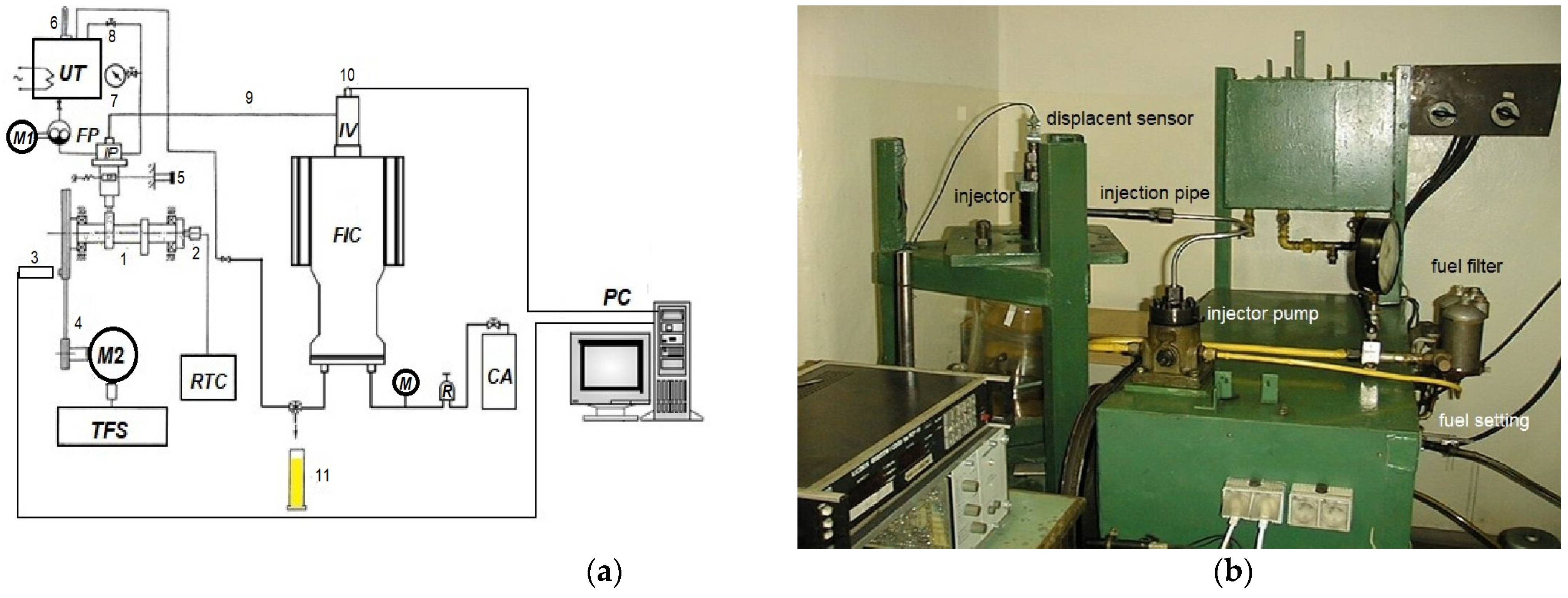
Figure 2. Diagram of the built modernized injector test stand (a) and view of the test stand (b): 1—camshaft, 2—rotation sensor, 3—camshaft position photo-optical sensor, 4—belt transmission, 5—fuel setting depth gauge, 6—thermometer, 7—pressure gauge, 8—throttle valve, 9—injection pipe, 10—eddy current displacement sensor, 11—measuring cup, FP—booster fuel pump, RTC—revolution and time counter, M1—the electric motor for pump drive, M2—the electric motor for the camshaft drive, CP—compressed air tank IP—injection pump, IV—injection valve, TFS—thyristor supply system, PC—computer, R—pneumatic reducer, FIC—fuel injection chamber.

Figure 2. Diagram of the built modernized injector test stand (a) and view of the test stand (b): 1—camshaft, 2—rotation sensor, 3—camshaft position photo-optical sensor, 4—belt transmission, 5—fuel setting depth gauge, 6—thermometer, 7—pressure gauge, 8—throttle valve, 9—injection pipe, 10—eddy current displacement sensor, 11—measuring cup, FP—booster fuel pump, RTC—revolution and time counter, M1—the electric motor for pump drive, M2—the electric motor for the camshaft drive, CP—compressed air tank IP—injection pump, IV—injection valve, TFS—thyristor supply system, PC—computer, R—pneumatic reducer, FIC—fuel injection chamber.

The mechanical part of this stand created a camshaft driven by a DC electric motor with a belt transmission. The calibration oil was supplied from the tank with the heater by gear pump and pressed by fuel filter to the injection pump.

Diagnostic signals were analyzed using the computer program signal analysis system (SAS). A preliminary process by selection in time, low-pass filtering, and synchronous averaging have been applied, and quantitative and qualitative analyses of spectra in the time and frequency domain have been applied [1,44]. This test stand was constantly developed and modernized.

The signal acquisition and analysis program allowed for analyzing a sequence of diagnostic signals originally presented in the cascaded form [1]. A cascade is a three-dimensional graph showing amplitudes as a function of time and sequence numbers. The functional, point and dimensionless estimates can be determined in this analysis option and summarized in the table. Functional estimates are the amplitude distribution function and probability function.

The mechanical part of this stand was formed by a camshaft driven by a DC electric motor through a belt transmission. Calibration oil was fed from a heater tank through a gear pump and pumped through a fuel filter to the injection pump. The tests were conducted for a conventional injection subsystem.

To identify the technical state, it is necessary to know the types and extent of wear and tear and the damage they have caused [6]. This study used simulation experiments, which have some advantages over numerical modeling. In the experimental studies undertaken in the past, there were significant limitations in that the components of the injection apparatus—new as well as one in service—have state features with random and widely varying values. Therefore, many manufactured samples of geometric and flow tests that met the requirements were selected [6]. Computer simulations were also conducted, but simplifying assumptions had to be made [45]. This made it possible to reduce the cost and time of testing and to analyze “isolated” damage, which in actual conditions of ICEs could encounter many difficulties.

The article formulates the following hypothesis: It is possible and expedient to use ML to classify and identify injectors’ technical states and develop a diagnostic symptom—the technical state model of a marine engine injector.

The micro- and macrostructure of fuel injection determine the combustion process. One element that determines the injection’s macrostructure is fuel distribution over time, called the injection course. The injection course is influenced by the design features of the injection subsystem [6], the fuel parameters, and the injection frequency [45].

3.2. Experimentally Simulated Technical States of the Injector

In this work, the effects of the control quantities and technical state of the following injector input quantities were studied:

-

Injection pump supply pressure p_f from 0.15 to 0.30 MPa;

-

Camshaft speed n from 150 to 450 rpm;

-

Fuel temperature at the injector inlet t_p = 20−50 °C;

-

Fuel dose control strip setting from 20 to 100%;

-

Changes in the tension of the spring, causing changes in the opening pressure of the injector needle in the range P_o = 15–30 MPa (the strength of the spring tension to achieve the required injector opening pressure);

-

Changes in the number of expensive holes in the injector nozzle i = 4 to 7;

-

Changes in the diameter of the spray holes d = 0.23 to 0.28 mm;

-

Changes in the average clearance at the leading part of the body and needle of the injector L_a;

-

Changing the maximum needle lift h_max;

-

Changes in the nozzle needle cone angle α = 59 to 61 °C.

The sum of the forces acting on the injector element $\sum F=F_1+F_2+F_3$ includes the force caused by the action of pressure p on the A component’s surface F₁ = pA, spring preload force F₂ = P_o, and spring deflection Δh force with k_sw stiffness F₃ = k_swΔh. Such values were dictated by the fact that these are essential input quantities for the conditions and state features, and by choice for the experimental plan [1,6]. In the first attempt to develop a network for solving a specific task, all variables that may be relevant should be included, as later at the design stage, this set is recommended to be reduced.

The state of the injection pump was investigated in a separate test. In this research, the state of the injection pump was assumed to be invariant. The supply pressure of the injection pump, p_f = 0.15 MPa, was the central value. Furthermore, the maximum inlet pressure to the injection pump could be 0.4 MPa. Thus, the following values of changes in fuel pressure before the injection pump p_f = 0.1; 0.15, 0.2, 0.25, and 0.3 MPa were established.

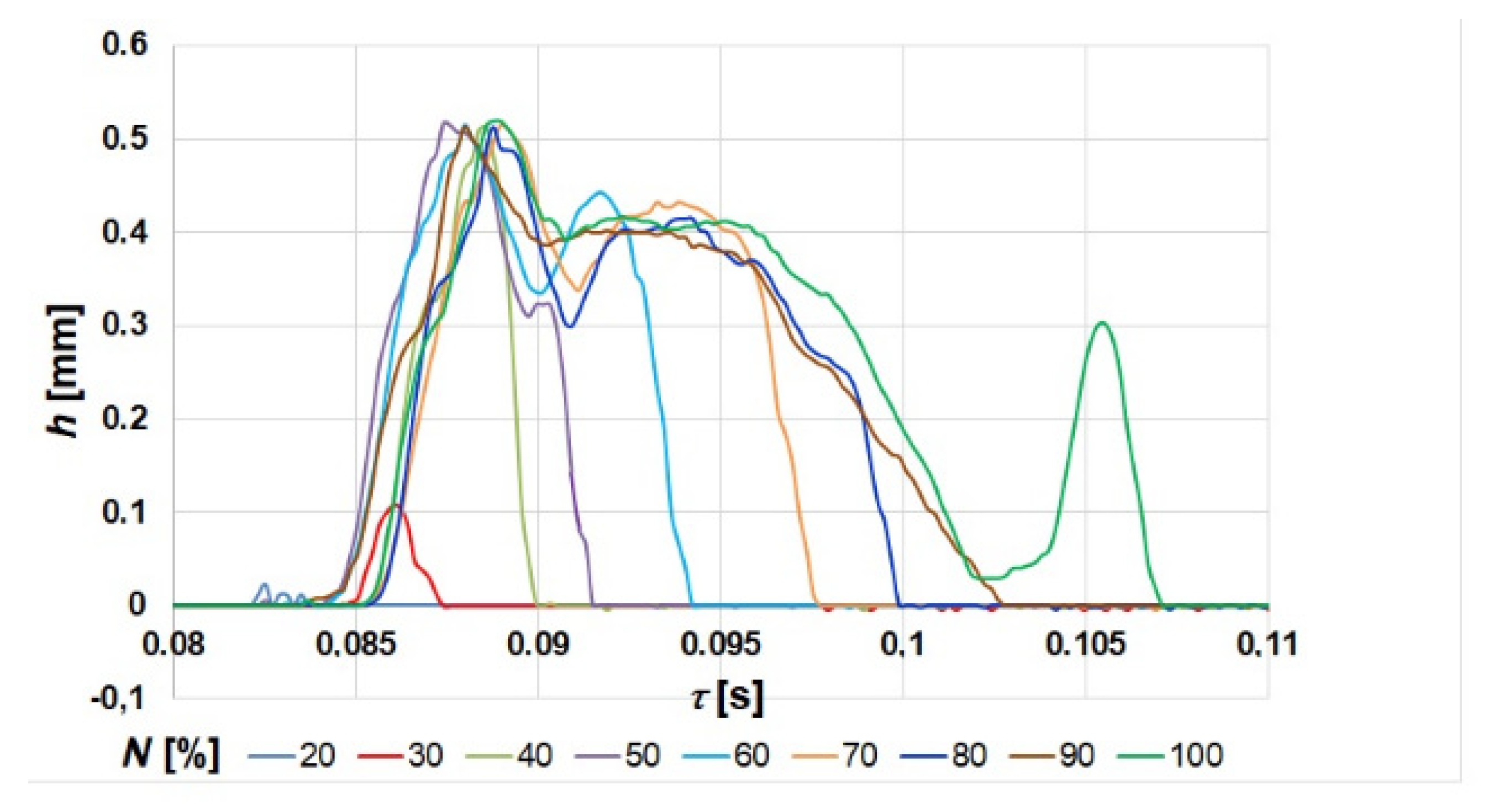
The fuel setting at which fuel injection does not occur is 20%. The maximum (100%) fuel setting was taken as the central value.The effect of fuel setting N on needle displacement waveform values h depending on time τ at constant injector opening pressure, is shown in Figure 3.

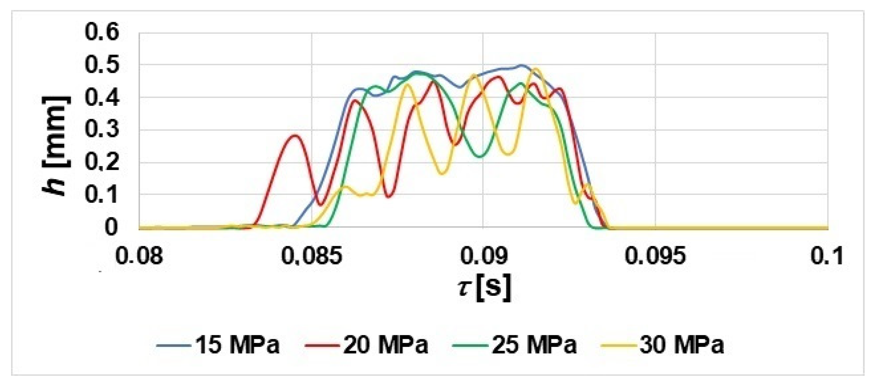
When the aforementioned research began and the injectors were purchased, the injector opening pressure of the AL20/24 type engine should be 25^+0.5 MPa. It represented a central value. As a result of the relaxation of the injector spring, the opening pressure changes (usually decreases). Therefore, a gradation of opening pressure every 5 MPa was adopted, from P_o = 15 MPa to P_o = 30 MPa. Changes in the opening pressure of the injector (derating) were simulated by changing the spring tension. This was achieved by screwing the adjustment screw into the injector body or unscrewing it. Two new 7 × 0.26 R (standard) injector nozzles were used for these tests, and the results were presented in the paper [6]. The effect of the injector opening pressure control on the time waveforms of vibration displacement signals is shown in Figure 4.

It can be observed from Figure 3 and Figure 4 that there were ripples in the nozzle displacement waveforms, especially for larger fuel settings.

3.3. Data Preparation for the Neural Network Model

The artificial NN model’s proper interpretation of injector failures depends on its ability to recognize characteristic symptoms of unfitness. For this purpose, sets consisting of different variants of single changes in state characteristics were developed while keeping constant the values in the state of unfitness of the others. However, the effect of combined damage when examining the nozzles of injectors in operation was also considered. In systems using ANNs, the more measurements, the more necessary data to train and validate the network.

The first important decision in building the network is determining which variables should be included and which cases should be collected. The displacement of the injector needle depends on the following input quantities that define the test conditions:

h = f(n, N, p_f, t_p)

(3)

where n is camshaft speed, N is fuel setting, p_f is the supply pressure of the injection pump, ρ is fuel density depending on the fuel type and the fuel temperature at the inlet t_p.

Fuel density depends on its temperature and pressure [6]. In experimental studies, it was assumed to be constant and determined at the inlet to the injection pump. In the experimental studies of the waveform of the injector nozzle needle displacement, the waveform of pressure in the combustion chamber was assumed constant, typically treated as continuous in the works. However, it was possible to supply compressed air at different pressures.

The steering values (fuel setting and rotational speed) were kept constant, and the state features were changed. Based on operational tests, the most common load was determined [1,46]. It was assumed that for unfitness, the listed state features receive a value of “0”, while when they fall within the tolerance field of the suitability state, they receive a value of “1”. Two sets of damage to the displacement waveforms of the nozzle needle were prepared. In reality, more features determine the condition of the injector nozzle, and the time waveforms of the pressure inside the nozzle sack are inadequate. However, in this research, they were assumed to be constant. These quantities appear in the model of the waveform of the nozzle needle displacement during fuel injection [45].

The input magnitudes determine the output magnitudes (simple and functional amplitude estimates), and thus the technical state of the injector S_t:

S_t = f(h_rms, h_aver, h_peak, K, C, I, B)

(4)

where h_rms is the root-mean-square values, h_aver is an average value, h_p is the peak value, K is the form factor, C is the peak factor, I is the impulsivity factor, and B is a dose of injected fuel.

Amplitude estimates are defined by the following measures [3]:

-

Root-mean-square values:

$$\tilde{h}(\theta )={\left[\frac{1}{T}{\int }_0^T{h}^2(\tau ,\theta )d\tau \right]}^{\frac{1}{2}}=h_{rms}(\theta )$$

(5)

-

Average value:

$$\overline{h}(\theta )=\frac{1}{T}{\int }_0^T\left|h(\tau ,\theta )\right|d\tau =h_{aver}(\theta )$$

(6)

-

Positive peak value:

$$\widehat{h}(\theta )=\mathit{max}\left[+h(\tau ,\theta )\right]=h_{peak}(\theta )$$

(7)

for 0 ≤ τ ≤ T.

Characterizing the quoted amplitude measures in terms of their sensitivity to the waveform of the process h(τ), it can be shown that each behaves differently. The rms value contains information about the energy of the signal under study, the average value represents the amplitude modulus of the signal, and the peak value contains information about the maximum values of the signal amplitudes.

The given definitions of amplitudes are instants of the stability and ergodic of the random processing h(τ) [3]. Thus, the selected dimensionless estimates of vibration processes, calculated from point measures according to the following relationships, were further used:

-

Shape factor:

$$K=\frac{\tilde{h}}{\overline{h}}$$

(8)

-

Peak factor:

$$C=\frac{\widehat{h}}{\overline{\tilde{h}}}$$

(9)

-

Impulsivity factor:

$$I=\frac{\widehat{h}}{\overline{h}}$$

(10)

The advantage of dimensionless discriminants is their qualitative nature, which gives versatility for various diagnostic signals.

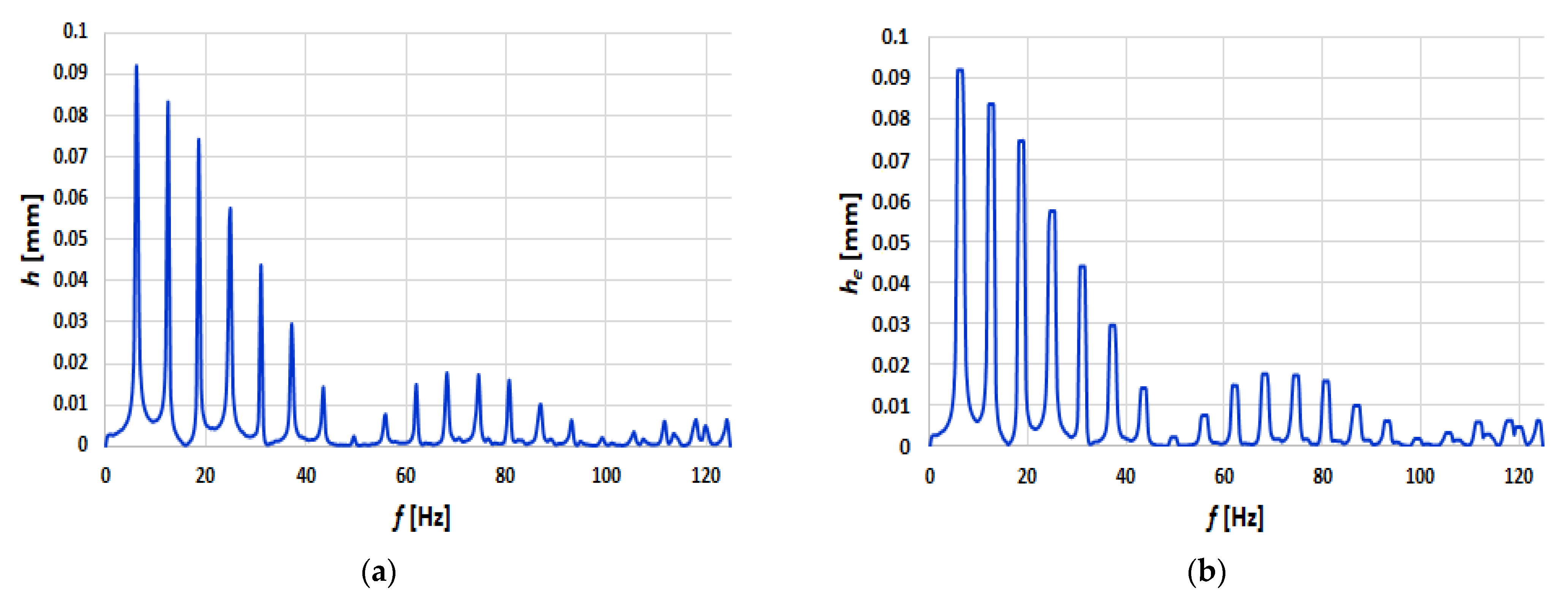
Analysis of the signals in the frequency domain showed that the most useful bandwidth was the frequency range of 0–125 Hz (Figure 5). These were polyharmonic signals with frequencies multiples of the rotational frequency nf_r. The amplitudes of the components of the spectra were read from the envelope.

Figure 5 shows that this was a polyharmonic line spectrum (discrete). Such a spectrum is represented by “spectral lines” with lengths proportional to the values of the H_i amplitudes of the individual components with frequencies f_o, 2f_o, 3f_o, …, nf_o. Other dimensions of signal analysis are described in the article [1].

Traditional frequency analysis is unsuitable for observing nonstationary signals’ properties with time-varying parameters. Slight changes in amplitudes and frequencies over time at the test stand outside the engine were caused by thermal processes. Thus, analyses were conducted using combined time–frequency representations of the signals. These analyses were performed as time–frequency (Figure 6) and time–scale [1] representations.

The time–frequency maps, apart from interesting visualization, did not yield significant differentiation using image color analysis [5].

3.4. Estimating Maximum Relative Errors of Diagnoses

The maximum errors made in the study of the application of the vibration displacement signal for diagnosing marine engine injectors were evaluated based on the most significant reading error, depending on the accuracy class of the measuring instruments and the size range of the measured quantities. The resulting maximum relative mistake of fuel injection parameters δ(F_i) was determined from the relation:

$$\delta \left(F_i\right)=100\%\sqrt{{\left(\frac{∆t_p}{t_p}\right)}^2+{\left(\frac{∆p_f}{p_f}\right)}^2+{\left(\frac{∆N}{N}\right)}^2+{\left(\frac{∆n}{n}\right)}^2+{\left(\frac{∆P_o}{P_o}\right)}^2}$$

(11)

where Δt_p is the absolute error of supply fuel temperature measurement, Δt_p is the absolute error of supply fuel pressure measurement, ΔN is the absolute error of fuel setting, Δn is the absolute error of camshaft speed measurement, and ΔP_o is the absolute error of injector opening pressure.

The values of relative maximum errors of individual processing elements of diagnostic signals in Figure 2 are shown in the article [44].

The total errors of the vibration displacement signal processing track and the subsequent determination of individual diagnostic parameters were qualitatively estimated. The relative maximum error of individual diagnostic signal measurement track S_d:

$$\delta \left(S_d\right)=100\%\sqrt{\left({\delta \left(F_i\right)}^2+{\delta \left(P_e\right)}^2\right)}$$

(12)

where d(P_e) is the relative maximum errors of individual processing elements of diagnostic signals.

The absolute root-mean-square error of the arithmetic mean of the diagnostic parameter, which was strongly influenced by the number of repeated measurements, can have the form:

$${\sigma }_s=\frac{\sigma }{\sqrt{n}}=\sqrt{\frac{1}{n(n-1)}{\sum }_{i=1}^n(D_{pi}-D_{pa}{)}^2}$$

(13)

where n is a number of measurements, σ is the standard deviation, D_pi is i-th measurement result of the diagnostic parameter, and D_pa is the average value of the diagnostic parameter.

The measurement method is burdened with systematic and random errors; they should be summed up according to the formula for the total error σ_t:

$${\sigma }_t(P_{dc})=\sqrt{{\left[{\sigma }_s\left(P_d\right)\right]}^2+\frac{1}{3}{\left[\sigma \left(D_p\right)\right]}^2}$$

(14)

Formula (14) is valid for absolute and relative errors and the results can be used for final presentations of diagnostic symptoms. The summed relative total errors of the point amplitude estimates and the amplitude components of the envelope spectra of firing pin displacement signals did not exceed ±3.6%.

4. Results

4.1. Neural Network Learning Results

Table 1. Examples of the input and output quantities used in the tests and the resulting technical states S_t for the fuel setting N.

Name	$\tilde{\mathit{h}}$	$\overline{\mathit{h}}$	$\widehat{\mathit{h}}$	Po	i	d	La	hmax	α	n	N	pf	tp	B	St
Unit	mm	mm	mm	MPa	–	mm	mm	mm	°	rpm	%	MPa	°C	mm3	–
7 × 0.23R	0.0850	0.0185	0.5414	25	7	0.23	0.0045	0.465	60.50	375	58	0.15	20	48.4	0
7 × 0.25R	0.0818	0.0172	0.511	25	7	0.25	0.0035	0.456	60.80	375	58	0.15	20	52.9	0
7 × 0.26R	0.0700	0.0162	0.485	25	7	0.26	0.0035	0.463	60.97	375	58	0.15	20	53.0	1
7 × 0.28R	0.0589	0.0130	0.506	25	7	0.28	0.0040	0.465	60.98	375	58	0.15	20	50.7	0

identifies the studied technical states S_t and, thus, the suitability of individual diagnostic parameters. Meeting very high criteria by the diagnostic symptoms made selecting the most useful among the diagnostic parameters possible.

Dimensionless estimates (8–10), resulting from point estimates (5–7), were discarded at the data preparation stage for learning.

Table 1 tells us that the results of the amplitude estimates were written as quantive outputs of the diagnostic signals used. The steering quantities and the state features were also reported as input quantities. The technical state for the cases shown was stored in the binary system as 1 for a suitability state and 0 for an unfit state.

At the outset of designing a network for solving a given task, one should include all variables that may be relevant so that the set can then be reduced. The rule recommends that the number of cases should be ten times the number of connections occurring in the network [47].

The first included only single faults, i.e., it included the following condition features:

-

(0,1,1,1,1,1,1,1,1,1,1,1,1,1,1,1,1)—inappropriate opening pressure of the injector;

-

(1,0,1,1, 1,1,1,1,1,1,1,1,1,1,1)—number of patented holes less than 7;

-

(1,1,0,1, 1,1,1,1,1,1,1,1,1,1,1)—diameter of the pinholes not within the tolerance field;

-

(1,1,1,1,0,1,1,1,1,1,1,1,1,1,1,1,1)—improper clearance in the guiding part of the body and the nozzle needle;

-

(1,1,0,1, 1,1,1,1,1,1,1,1,1,1)—needle cone angle not within the tolerance field;

-

(1,1,1,1,1, 1,1,0,1,1,1,1,1,1)—incorrect camshaft rotational speed;

-

(1,1,1,1, 1,1,1,1,0,1,1,1,1)—incorrect fuel setting;

-

(1,1,1,1, 1,1,1,1,1,0,1,1)—incorrect injection pump supply pressure;

-

(1,1,1,1,1, 1,1,1,1,1,1,0,1)—improper fuel temperature;

-

(1,1,1,1,1, 1,1,1,1,1,1,1,1,1,0)—incorrect dose of fuel pumped through the nozzle.

The second set additionally consisted of combined technical states. That is, its scope included the example operated injector nozzles: (1,1,1,0, 1,1,1,1,1,1,0).

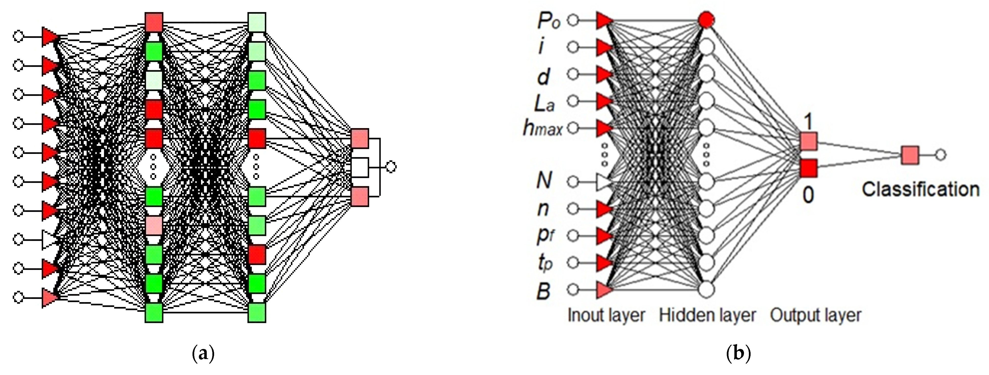
Figure 7a shows the architecture of an example of a raw MLP network, and Figure 7b shows the network with descriptions of inputs, layers, and outputs. The network architectures were made in the Statistica 7 computer program.

The network response mandates additional interpretation in classification networks to establish recognition based on which output layer neuron presents the highest signal parameter value.

In the diagnostic study, a large amount of data was collected, describing the diagnostic objects’ inputs, states, and outputs. These data were initially classified by assigning technical state classes to them. Experimental data collected are declarative knowledge carriers subjected to ML in the Statistica 13.3 and MATLAB R2022a environment. All benchmark data and graded changes of single state characteristics and quantities defining test conditions were selected as a learning set, accounting for 63.26%.

ML in classification is the issue of determining to which set of technical state categories newly observed data belong. Assignment to a category was made based on previously entered training data whose membership in the class has been determined.

The injector was at full ability and not unfit for graded changes in fuel temperature and injection pump supply pressure. All data from new injectors were taken as validation data (18.37%). The test set for fuel setting 58 and 100% accounted for 18.37%. The global sensitivity measure shown in

Table 2. A global measure of the sensitivity of input quantities for the sample: learning, test, validation.

Item	Network Name	n	La	α	B	hrms	Po	N	i	pf	haver	hpeak	hmax
1	MLP 14-5-2	1.051	1.293	1.248	1.136	1.848	1.161	1.084	1.315	1.090	1.145	0.996	1.103
2	MLP 14-13-2	2.819	1.748	1.845	1.754	1.473	1.274	1.549	1.191	1.218	1.195	1.173	1.100
3	MLP 14-11-2	2.314	1.963	1.656	1.551	1.313	1.265	1.332	1.160	1.129	1.216	1.170	1.125
4	MLP 14-6-2	2.077	1.698	1.880	1.679	1.605	1.634	1.436	1.655	1.394	1.196	1.359	1.046
5	MLP 14-8-2	1.844	1.272	1.228	1.260	1.077	1.127	1.146	1.102	1.101	1.024	1.059	1.074
6	MLP 14-7-2	1.877	1.742	1.603	1.560	1.094	1.306	1.104	1.171	1.189	1.125	1.083	1.068
	Average	1.997	1.619	1.577	1.490	1.402	1.295	1.275	1.266	1.187	1.150	1.140	1.086

assesses the data’s variability. The MLP 14-5-2 network contains 14 input neurons, 5 to 13 neurons in the hidden ply, and two in the output ply.

The susceptibility of diagnostic parameter values was be determined by the sensitivity coefficient s_c defined by the formula:

$$s_c=\frac{y_{imax}-y_{imin}}{\overline{y}}$$

(15)

where y_imax is the maximum quality of the measured diagnostic parameter, y_imin—the minimum quality of the measured diagnostic parameter, $\overline{y}$ is the average value of a given diagnostic parameter in a group of observations.

It can be observed from Table 2 that the highest sensitivity is the camshaft speed n, and the lowest sensitivity is the temperature of the fuel supply t_p for these data. Sensitivity analysis informs the utility of the input variables, that is, the practical usefulness.

4.2. Analysis and Interpretation of Test Results

The purpose of the classification is to assign the case to one of the predefined classes [47,48]. Each of the predicted classes corresponds to one neuron in the output layer. The outputs for these data are two-state in nature. The information is presented in the form of classification statistics. The summary results are recorded in

Table 3. Summary of active networks.

Network ID	Network Name	Learning Quality	Testing Quality	Validation Quality	Error Function
1	MLP 14-5-2	92.06349	82.35294	100.0000	SOS
2	MLP 14-13-2	93.65079	88.23529	100.0000	Entropy
3	MLP 14-11-2	93.65079	94.11765	100.0000	SOS
4	MLP 14-6-2	90.47619	94.11765	94.1176	SOS
5	MLP 14-8-2	88.88889	94.11765	94.1176	Entropy
6	MLP 14-7-2	90.47619	94.11765	94.1176	Entropy

.

The best network turned out to be No. 3. From Table 3, there is a high quality of learning, testing, and validation (generally above 90%), and for individual networks, even 100%. However, many incorrect classifications exist, up to 6 for the MLP 14-6-2 network (

Table 4. Fragment of the confusion matrix in the classification summary for the sample: learning, test, validation.

Network ID	Network Name	Classification Summary	State 0	State 1	State All
1	MLP 14-5-2	Correct (%)	95.65217	82.14286	91.75258
		Incorrect (%)	4.34783	17.85714	8.24742
2	MLP 14-13-2	Correct (%)	97.10145	85.71429	93.81443
		Incorrect (%)	2.89855	14.28571	6.18557
3	MLP 14-11-2	Correct (%)	95.65217	92.85714	94.84536
		Incorrect (%)	4.34783	7.14286	5.15464

). This high proportion of mistakes may be due to the correlation of diagnostic parameters with measured technical states. They form very accurate relationships (k > 0.900), accurate relationships (k > 0.700), and only in a few cases, significant relationships (k > 0.500). The minor confusion in the matrix in the classification summary was found in the MLP 14-11-2 network (Table 4).

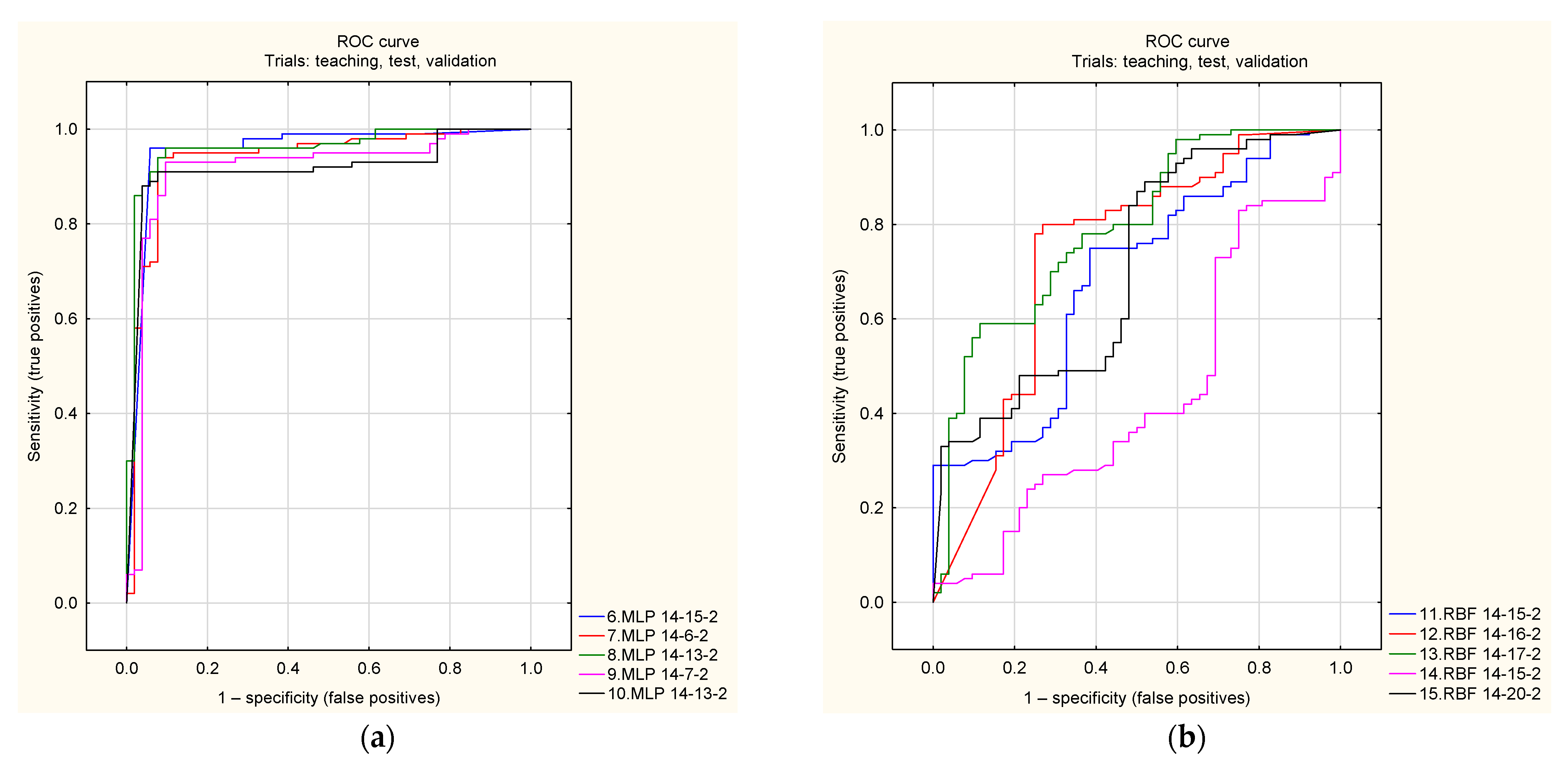
Another measure of the quality of the network as a classifier is the receiver operating characteristic curve (ROC), which shows the cumulative specificity (false positives) on one axis and sensitivity (true positives) on the other. A classifier groups a set of features into decision groups so that all data located in this subspace corresponds to a distinguished group (class). The boundary values in these sets are called decision-marker subsurfaces. A decision boundary is an area in the feature space where the corresponding criterion functions (class membership functions) have the same value.

The closer the area under the curve (AUC) is to unity, the better the classifier’s quality. As can be observed from the ROC and AUC values (Figure 8), the results obtained by the MLP network are excellent and slightly worse for the RBF.

Determining the area under the ROC graph from the allegation is the area for the ideal model (the area of a square with side 1). The area under ROC (AUROC) denotes the probability that the predictive model under study is higher (the value of the correlated element of the positive class than the random element of the accepted class).

Table 5. ROC plots and thresholds for learning, testing, and validation for the top six networks.

Network ID	Area and ROC Threshold for Sampling: Teaching, Testing, Validation
	MLP 14-5-2	MLP 14-13-2	MLP 14-11-2	MLP 14-6-2	MLP 14-8-2	MLP 14-7-2
1	0.932712	0.972050	0.966874	0.966874	0.965839	0.965321
2	0.530628	0.682748	0.551377	0.551377	0.434712	0.482753

shows the areas and ROC thresholds for learning, testing, and validation for the top six networks, from which it can be seen that the additional common one is MLP 14-13-2 network two.

From the presented results of the experimental study of the nozzle needle displacement signals of the execution of classification using the ANN in the Statistica 13 environment, the suitability for the state recognition is evident. Tests were also carried out for more measurement data by increasing the cases with frequency domain analysis for the first three components. Tests were also carried out for other signals [17] in various analysis domains (including wavelet transforms) and using the MATLAB R2022a computer program, and similar satisfactory results were obtained. The classification learner was used to train models that classify data. It belongs to the group of supervised learning. This application allows to select features, examine data, train models, and determine validation and testing.

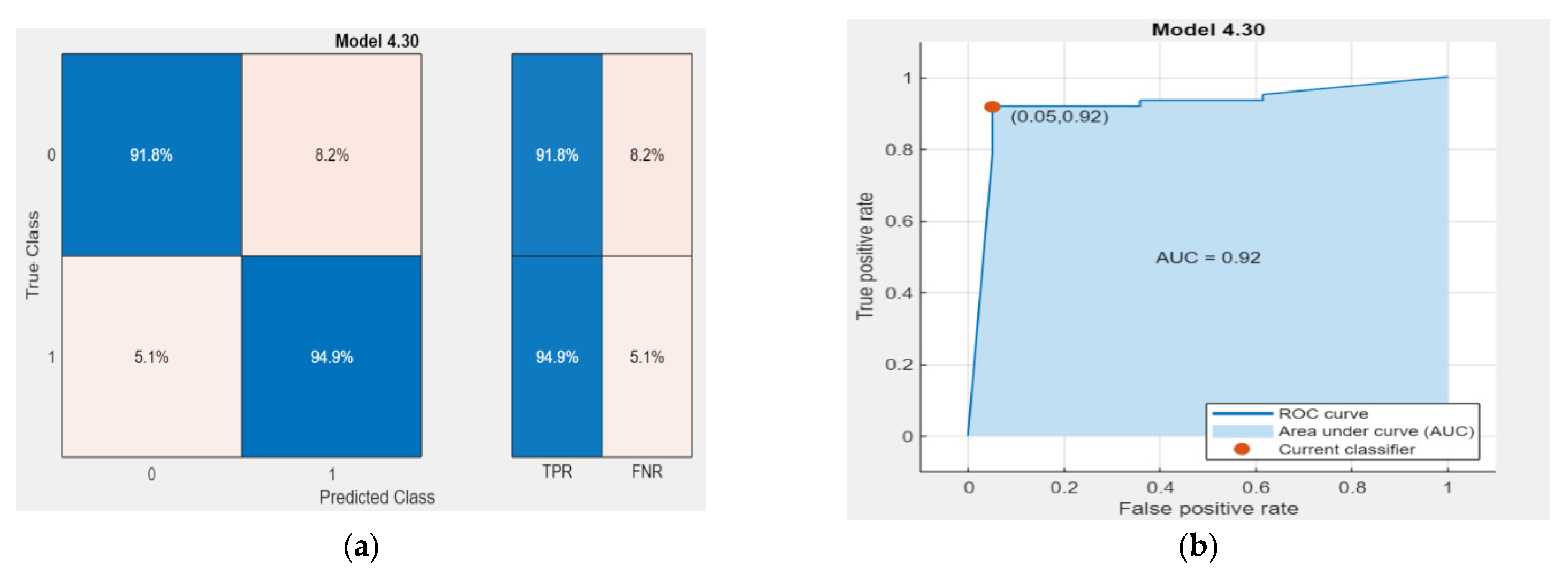
Figure 9a shows the different models used in the classification and their corresponding validation accuracies in MATLAB 2022a. The highest validation accuracies were obtained from models 4.24 of the Subspace KNN (k-nearest neighbor) = 95.0%. The algorithm was also trained using standard hyperparameters, and optimization methods were used. Figure 9b shows the minimum classification error for model 5.

The Statistica computer program in the automatic NN application has several options for learning MLP networks. These are Broyden–Fletcher–Goldfarb–Shanno (BFGS), coupled gradients, and the fastest gradient algorithm. The methods mentioned are optimization methods, and in this article, all MLP networks have the BFGS algorithm. Similar capabilities were in Matlab 2022a.

Figure 10a shows the classification learner matrix for the tree-layer NN. The matrix shows the percentage of observations and the proportion of correctly classified data (blue diagonal), and the cream-colored diagonal represents incorrectly classified data. Quality measures of a binary classifier are the “true positive rate” (TPR) to the “false positive rate” (FPR) [37,46]. Specificity (True Negative Rate) is the probability of detecting a passable state provided that there is one:

$$TNR=\frac{TN}{TN+EP}$$

(16)

where TN is negative cases the classifier detects as negative, and FP is negative cases falsely detected as positive. The false positive rate (false alarm) is the ratio of the number of cases falsely classified as an unfit condition to all cases:

$$FA=FPR=\frac{EP}{TN+EP}$$

(17)

Meanwhile, Figure 10b shows the ROC curve, which gives the ratio of correctly classified observations to incorrect ones for different classification thresholds.

The TPR (true positive rates) matrix represents the percentage of correctly classified observations for fitness class 1, and the FNR (false negative rates) represents the percentage of incorrectly classified observations for abnormal class 0. Running multiple variants of the tests for Statistica 13 and MATLAB R2022a programs and other signal analysis domains will help select the optimal solution.

5. Discussion

Some authors have studied the effect of operating conditions of the facility, and here, data have been collected over the entire range of variation in the parameters determining the conditions.

Successful results encourage further research using pressure signals in the fuel injection subsystems, in-cylinders of marine ICEs, and speed and vibration acceleration. In addition to analyses in the time, amplitude, and frequency domains, further time–frequency analyses, wavelet transforms, and other advanced analyses of diagnostic signals are being conducted.

The authors’ contribution is also the execution of the research in the broad area of planned experimental studies. The diagnostic parameters used in the amplitude and frequency domain were related to the conducted measurements of the geometric and flow features of the technical state. Thus, deterministic models were obtained. Classifications carried out using NNs and two computer programs confirmed the nonrandomness of good validation and testing qualities.

Future research should also use diagnostic parameters recorded on marine ICEs under operating conditions. Operational tests have been carried out under natural conditions on more than 100 marine engines driving generators under marine ship conditions using vibration displacement signals and other working and residual processes.

6. Conclusions

NNs help identify typical faults in diagnosing marine engine injectors using displacement vibration signals. The study analyzed 10,000 types of networks, and MLP networks were selected from which the best one can be identified. Satisfactory quality of learning, validation, and testing by close and very close relationships with the values of diagnostic parameters in the studied ranges of variability were obtained. Test quality reached more than 90% using selected NNs of Statistica and MATLAB environments, and for the MLP networks, validation quality was 100%.

The experimental data of learning, validation, and testing sets in manual and random ways influenced the results. Higher qualities were obtained for random selection. The contribution of the present study to state of the art is the inclusion of several properties of the state features measured experimentally for model and randomly worn nozzles.

In further work, efforts should be made to reduce errors in classifying technical states by selecting insensitive data and matching hyperparameters when learning NNs.

7. Patents

Monieta, J. Method and device for diagnosing injectors. Patent of the Patent Office of the Republic of Poland WUP 09/08 2008, No. 199362B1, pp. 1–6.

References

1. Monieta, J. Selection of diagnostic symptoms and injection subsystems of marine reciprocating internal combustion engines. Appl. Sci. 2019, 9, 1540. [Google Scholar] [CrossRef]
2. Klimkiewicz, M. Application of neural networks in the diagnostics of the fuel apparatus of compression-ignition engines. Agricult. Eng. 2005, 8, 153–160. [Google Scholar]
3. Żółtowski, B.; Cempel, C. Elements of the Theory of Technical Diagnostics. In Engineering of Diagnostics Machines; Society of Technical Diagnostics: Bydgoszcz, Poland, 2004; pp. 17–525. [Google Scholar]
4. Marine Engine IMO Tier II and Tier III Programme. Engineering for Future—Since 1758. MAN Diesel & Turbo. 2015. Available online: https://www.man-es.com/marine/products/planning-tools-and-downloads/marine-engine-programme (accessed on 16 January 2023).
5. Monieta, J. Application of image color analysis for the assessment of injector nozzle deposits in internal combustion engines. SAE Int. J. Fuels Lubr. 2022, 2, 1–12. [Google Scholar] [CrossRef]
6. Monieta, J.; Łukomski, M. Methods and means of estimation of technical state features of the marine diesel engines injector nozzles type Sulzer 6AL20/24. Scient. J. Mar. Univ. Szczecin 2005, 5, 383–392. Available online: https://wydawnictwo_am_szczecin_plzeszyty-naukowepobierzcategory19-zn-5-77-omiuo-2005 (accessed on 15 March 2023).
7. Klimkiewicz, M. Neural model for localization of damage to injection pumps. Agricult. Eng. 2008, 1, 159–164. [Google Scholar]
8. Pantelelis, N.G.; Kanarachos, A.E.; Gotzias, N.D.; Papandreou, N.; Gu, F. Combining vibrations and acoustics for the fault detection of marine diesel engines using neural networks and wavelets. In Proceedings of the 14th International Congress on Condition Monitoring and Diagnostic Engineering Management (COMADEM 2001), Manchester, UK, 4–6 September 2001; pp. 649–656. [Google Scholar]
9. Haukin, S. Neural Networks, A Comprehensive Foundation; Macmillan College Publishing Company: New York, NY, USA, 2000. [Google Scholar]
10. Kecman, V. Support Vector Machines, Neural Networks and Fuzzy Logic Models; MIT Press: Cambridge, MA, USA, 2001. [Google Scholar]
11. Osowski, S. Neural Networks for Information Processing; Publishing House of the Warsaw University of Technology: Warsaw, Poland, 2006. [Google Scholar]
12. Schoellkopf, B.S.; Smola, A.J. Learning with Kernels; MIT Press: Cambridge, MA, USA, 2002. [Google Scholar]
13. Rutkowski, L. Methods and Techniques of Artificial Intelligence; National Scientific Publishing House: Warsaw, Poland, 2012. [Google Scholar]
14. Brzeżański, M.; Golomb, P. Application of the neural network method for the analysis of particulate emissions in the exhaust of CI and SI engines. Combust. Eng. 2009, SC1, 331–337. [Google Scholar]
15. Jankowski, M.; Kwidziński, M. Application of Neural Network for Automatic Classification of Injection Apparatus; Congress of Technical Diagnostics: Gdansk, Poland, 1996; pp. 312–318. [Google Scholar]
16. Lewicki, P.; Hill, T. Statistics Methods and Applications Book; StatSoft: Tulsa, OK, USA, 2011. [Google Scholar]
17. Monieta, J.; Choromański, T. The application of artificial intelligence to identification of typical damages of marine diesel engines injectors. Diagnostyka 2008, 4, 139–144. [Google Scholar]
18. Sitnik, L. Neural networks in diesel engine control. In Proceedings of the PTNSS Congress—2005, The Development of Combustion Engines, Szczyrk, Poland, 25–28 September 2005; pp. 1–15. [Google Scholar]
19. Cheliotis, M.; Lazakis, I.; Cheliotis, A. Bayesian and machine learning-based fault detection and diagnostics for marine applications. Offshor. Struct. 2022, 1, 1–13. [Google Scholar] [CrossRef]
20. Raptodimos, Y.; Lazakis, I. Using artificial neural network-self-organising map for data clustering of marine engine condition monitoring applications. Ship. Offshor. Struct. 2018, 13, 649–656. [Google Scholar] [CrossRef]
21. Wang, R.H.; Chen, H.; Guan, C. Random convolutional neural network structure: An intelligent health monitoring scheme for diesel engines. Measurement 2021, 171, 108786. [Google Scholar] [CrossRef]
22. Xu, X.; Zao, Z.; Xu, X.; Yang, J.; Chang, L.; Yan, X.; Wang, G. Machine learning-based wear fault diagnosis for marine diesel engine by fusing multiple data-driven models. Knowl. Based Syst. 2020, 190, 105324. [Google Scholar] [CrossRef]
23. Zhang, J.; Zhang, D.; Shen, G.; Yang, J. Research on fault diagnosis of marine diesel engine based on probabilistic neural network optimized by quantum genetic algorithm. In Proceedings of the 2021 IEEE 4th International Conference on Automation, Electronics and Electrical Engineering (AUTEEE), Shenyang, China, 19–21 November 2021; pp. 729–733. [Google Scholar]
24. Abramek, K.; Osipowicz, T.; Mozga, Ł. The use of neural network algorithms for modeling injection doses of modern fuel injectors. Combust. Eng. 2021, 185, 10–14. [Google Scholar] [CrossRef]
25. He, Y.; Rutland, C.J. Application of artificial neural networks in engine modeling. Int. J. Eng. Res. 2004, 5, 281–296. [Google Scholar] [CrossRef]
26. Pawletko, R. The Use of neural networks for the faults classification of a marine diesel engine fuel injection system. Glob. J. Eng. Educ. 2005, 9, 143–148. [Google Scholar]
27. Pawletko, R. Using a neural network to diagnose selected malfunctions of a marine engine. Diagnostyka 2002, 27, 43–47. [Google Scholar]
28. Brzozowski, K.; Nowakowski, J. Application of artificial neural network to identify the working cycle model of compression ignition engine. In Proceedings of the First International Congress on Combustion Engines. PTNSS Congress—2005. The Development of Combustion Engines, Szczyrk, Poland, 25–28 September 2005; pp. 1–9. [Google Scholar]
29. Logan, K.; Inozu, B.; Roy, P.; Hetet, J.F.; Chesse, P.; Tauzia, X. Real-time marine diesel engine simulation for fault diagnosis. Mar. Technol. Snam. News 2002, 39, 21–28. [Google Scholar] [CrossRef]
30. Mesbahi, E. An intelligent sensor validation and fault diagnostic technique for diesel engines. J. Dyn. Sys. Measur. Contr. Trans. ASME 2001, 123, 141–144. [Google Scholar] [CrossRef]
31. Ramteke, S.M.; Chelladurai, H.; Amarnath, M. Diagnosis of liner scuffing fault of a diesel engine via vibration and acoustic emission analysis. J. Vib. Eng. Technol. 2019, 8, 815–833. [Google Scholar] [CrossRef]
32. Wang, R.H.; Chen, H.; Guan, C. A Bayesian inference-based approach for performance prognostics towards uncertainty quantification and its applications on the marine diesel engine. ISA Trans. 2021, 118, 159–173. [Google Scholar] [CrossRef]
33. Garczynska, I.; Tomczak, A.; Stepien, G.; Kasyk, L.; Slaczka, W.; Kogut, T. Applicability of machine learning for vessel dimension survey with a minimum number of common points. Appl. Sci. 2022, 12, 3453. [Google Scholar] [CrossRef]
34. Zhu, J.Y. Marine Diesel engine condition monitoring by use of bp neural network. In Proceedings of the International Multi Conference of Engineers and Computer Scientists Vol II IMECS 2009, Hong Kong, 18–20 March 2009; pp. 1–4. [Google Scholar]
35. Klinkmann, J.E. Wärtsilä Asset Diagnostic Configurator. Bachelor’s Thesis, Novia University of Applied Science, Vaasa, Finland, 2019. [Google Scholar]
36. Wang, R.H.; Chen, H.; Guan, C. DPGCN model: A novel fault diagnosis method for marine diesel engines based on imbalanced datasets. IEEE Trans. Instrum. Meas. 2023, 72, 3504011. [Google Scholar] [CrossRef]
37. Shahid, S.M.; Ko, S.; Kwon, S. Real-Time Classification of Diesel Marine Engine Loads Using Machine Learning. Sensors 2019, 19, 3172. [Google Scholar] [CrossRef] [PubMed]
38. Cheliotis, M.; Lazakis, I.; Theotokatos, G. Machine learning and data-driven fault detection for ship systems operations. Ocean Eng. 2020, 216, 107968. [Google Scholar] [CrossRef]
39. Monieta, J. Diagnosing cracks in the injector nozzles of marine internal combustion engines during operation using vibration symptoms. Appl. Sci. 2023, 13, 9599. [Google Scholar] [CrossRef]
40. Kowalski, J.; Krawczyk, B.; Woźniak, M. Fault diagnosis of marine 4-stroke diesel engines using a one-vs-one extreme learning ensemble. Eng. Appl. Artif. Intell. 2017, 57, 134–141. [Google Scholar] [CrossRef]
41. Ramteke, S.M.; Chelladurai, H.; Amarnath, M. Diagnosis and Classification of Diesel Engine Components Faults Using Time-Frequency and Machine Learning Approach. J. Vib. Eng. 2022, 10, 175–192. [Google Scholar] [CrossRef]
42. Adamkiewicz, A.; Nikonczuk, P. An attempt at applying machine learning in diagnosing marine ship engine turbochargers. Mainten. Reliab. 2022, 24, 795–804. [Google Scholar] [CrossRef]
43. Zhao, H.; Mao, Z.; Chen, K.; Jiangn, Z. An intelligent fault diagnosis method for a diesel engine valve based on improved wavelet packet-Mel frequency and convolutional neural network. In Proceedings of the International Conference on Sensing, Diagnostics, Prognostics, and Control (SDPC) 2019, Beijing, China, 15–17 August 2019; pp. 354–359. [Google Scholar] [CrossRef]
44. Monieta, J. Method and a device for testing the friction force in precision pairs of injection apparatus of the self-ignition engines. Energies 2022, 15, 6898. [Google Scholar] [CrossRef]
45. Monieta, J.; Kasyk, L. Optimization of design and technology of injector nozzles in terms of minimizing energy losses on friction in compression ignition engines. Appl. Sci. 2021, 11, 7341. [Google Scholar] [CrossRef]
46. StatSoft, Inc. Electronic Statistic Textbook; StatSoft: Tulsa, OK, USA, 2013; pp. 1984–2011. ISBN 13: 9781884233593. [Google Scholar]
47. Tadeusiewicz, R.; Szaleniec, M. Lexicon of Neural Networks; Publisher of the Project Science Foundation: Wrocław, Poland, 2015. [Google Scholar]
48. Çelebi, K.; Uludamar, E.; Tosun, E.; Yıldızhan, Ş.; Aydın, K.; Özcanlı, M. Experimental and artificial neural network approach of noise and vibration characteristic of an unmodified diesel engine fuelled with conventional diesel, and biodiesel blends with natural gas addition. Fuel 2017, 197, 159–173. [Google Scholar] [CrossRef]
Figure 1. Schematic of an MLP network with two hidden layers.
Energies 16 06898 g001
Figure 3. The effect of fuel setting N on the values of the needle displacement waveform h depends on the time τ at a constant injector opening pressure Po = 25 MPa.
Energies 16 06898 g003
Figure 4. The effect of injector tension force Po on the values of the nozzle lift waveform h as a function of time τ.
Energies 16 06898 g004
Figure 5. Example spectrum for fuel setting N = 58% and injector nozzle with a hole diameter d = 0.28 mm (a) and spectrum envelope (b).
Energies 16 06898 g005
Figure 6. Time–frequency analysis of the needle vibration displacement signal for an injector opening pressure of 30 MPa and at a fuel setting of 58%.
Energies 16 06898 g006
Figure 7. The architecture of an example raw MLP network (a) and with descriptions of inputs, layers, and outputs for GRNN network (b).
Energies 16 06898 g007
Figure 8. Receiver operating characteristics curve (ROC) for five MLP (a) and RBF (b) networks receiver.
Energies 16 06898 g008
Figure 9. The different models used in classification and their corresponding validation accuracies in MATLAB (a) and minimum classification error for model 5 (b).
Energies 16 06898 g009
Figure 10. Example classification learner (a) and classification matrix ROC curve 10 (b) for the 4.30 model of the three-layer NN for parameters in the amplitude and frequency domain in MATLAB software.
Energies 16 06898 g010