Simple Strategy for Torque Ripple Minimization in Switched Reluctance Motor Drives

Abstract

This article proposes a new simulation strategy to support the calculation of the angular interval of the current supply to minimize the torque ripple in switched reluctance machines, focusing on the motor working condition. Supposing the best angular interval is strongly linked to the working condition of the machine, a formula is needed to calculate the boundary angles of the intervals of the current supply for each phase, starting from real-time speed and electromagnetic torque. Starting from the dataset of simulations made with this new strategy, linear regression was used to train a model that computes useful formulas. The aim of this research is to show how the application of simple calculations allows torque ripple and power losses to be reduced, i.e., RMS phase currents, without altering the geometry of the machine. Simulations on a virtual four-phase 8/6 SRM are carried out to verify the model’s feasibility and effectiveness, even though this strategy can be easily applied to all other configurations of SRMs.

1. Introduction

Switched reluctance machines (SRMs) are currently being studied by many engineers and researchers because of some features which make them cheap: a simple mechanical structure and geometry, no permanent magnets, and concentrated windings on stator poles only.

Although cheap and robust, many disadvantages prevent these machines from spreading in the global market. First of all, a high value of torque ripple implies relevant acoustic noise and rapid wear of bearings. To increase SRMs’ lifetimes, expensive bearings are needed, so the advantage of the cheap mechanical structure is lost. In addition, compared with high-performance brushless motors with the same rated torque, switched reluctance machines are typically bigger.

The main research topics for SRMs deal with improving their efficiency and reducing the torque ripple, vibrations, and acoustic noise. In recent years, many studies on these machines have focused on accurate physical modeling and on high-performance control strategies. In [1], a simple model of a standard switched reluctance machine is obtained considering the magnetization characteristics of iron and the geometry of the machine (the number of stator and rotor poles). In [2], the main Fourier harmonics are used for mathematical expressions of the torque and phase inductances, taking into account non-linear features which appear when a stator salient pole and a rotor pole are going to overlap. In [3], the researchers propose a methodical process to calculate unknown machine parameters by introducing some project constraint conditions, which cut out some design degrees of freedom. In [4], comparisons between analytical predictions and a finite element analysis (FEA) are made to identify the optimal angular position of the rotor when the incoming phase has to be switched on (angle_on) to maximize the torque peak. In [5], the finite element method (FEM) is used to implement a two-dimensional (2-D) thermal analysis on a double-stator SRM, a novel type of machine for which there is still limited information about heat losses.

In [6], some analytical models are used to try to predict non-linear characteristics, and their effectiveness is proved through comparison with FEM calculations and experimentation; this article confirms that we can substitute long simulation times (experimentation and FEM) with faster simulations based on mathematical models, without a significant loss of accuracy.

Finding an effective analytical model for all SRMs is difficult, it is easier to adapt torque and inductance expressions from one case study so new control schemes and strategies can be developed. With this aim, a large number of studies have been carried out on 12/8 SRM machines, in order to maximize machine efficiency.

In [7], a comparison between a single-phase and a three-phase SRM is shown, which is useful for understanding that the similarities and differences between different configurations of this type of machine are not large.

In [8], a switched reluctance machine being used as generator is shown, pointing out that a different power electronics is needed to avoid problems linked to high back-electromagnetic forces in generator working conditions.

In [9], a novel modular four-level power converter is proposed in order to provide control flexibility and enhance torque ripple reduction capability. This work was carried forward in [10] to improve machine performance even more.

In [11], an optimized direct instantaneous torque control (DITC) is applied to change the angular position of the rotor, where the incoming phase is switched off (angle_off) through an algorithm which adapts its value to obtain the minimum torque ripple. A less complex algorithm to change the boundary angles of the current supply is shown in [12], where a simple calculation made by the microcontroller in real time provides the angle_off value (mechanical angle that determines the start of discharge transient) and the angle_on value (mechanical angle that determines the start of the charge transient) so that the torque ripple is minimized. Although it is not always possible to reach the plateau of the desired constant phase current value in a short time, this work is considered as extremely valid. In [13], a vibration comparison between a variable flux machine and an SRM is shown through the current superimposition mode. Vibrations are one of the most relevant issues of these kind of machines, so are always taken into account to evaluate the effectiveness of the research.

Through the years, many control strategies have been proposed trying to maximize performance in each detail of machine working: in [14], some computations through torque sharing functions (TSFs) were performed in order to reduce the amount of current sensors on the power electronics, and obtain similar performance; in [15], a capacitor was inserted into the power electronics scheme, chosen as a compromise between strong dynamics and a high voltage peak.

In this article, a new simulation strategy approach is proposed in order to find a smaller angular interval to supply current to each phase in order to minimize the torque ripple: this corresponds to the angular rotor positions where the current starts and ends while charging a certain phase. Once these are found, the work is not over: a huge table, which links each working condition with the right angular interval, is necessary, and then it should be stored in the microcontroller. However, this would be very expensive in terms of computational memory.

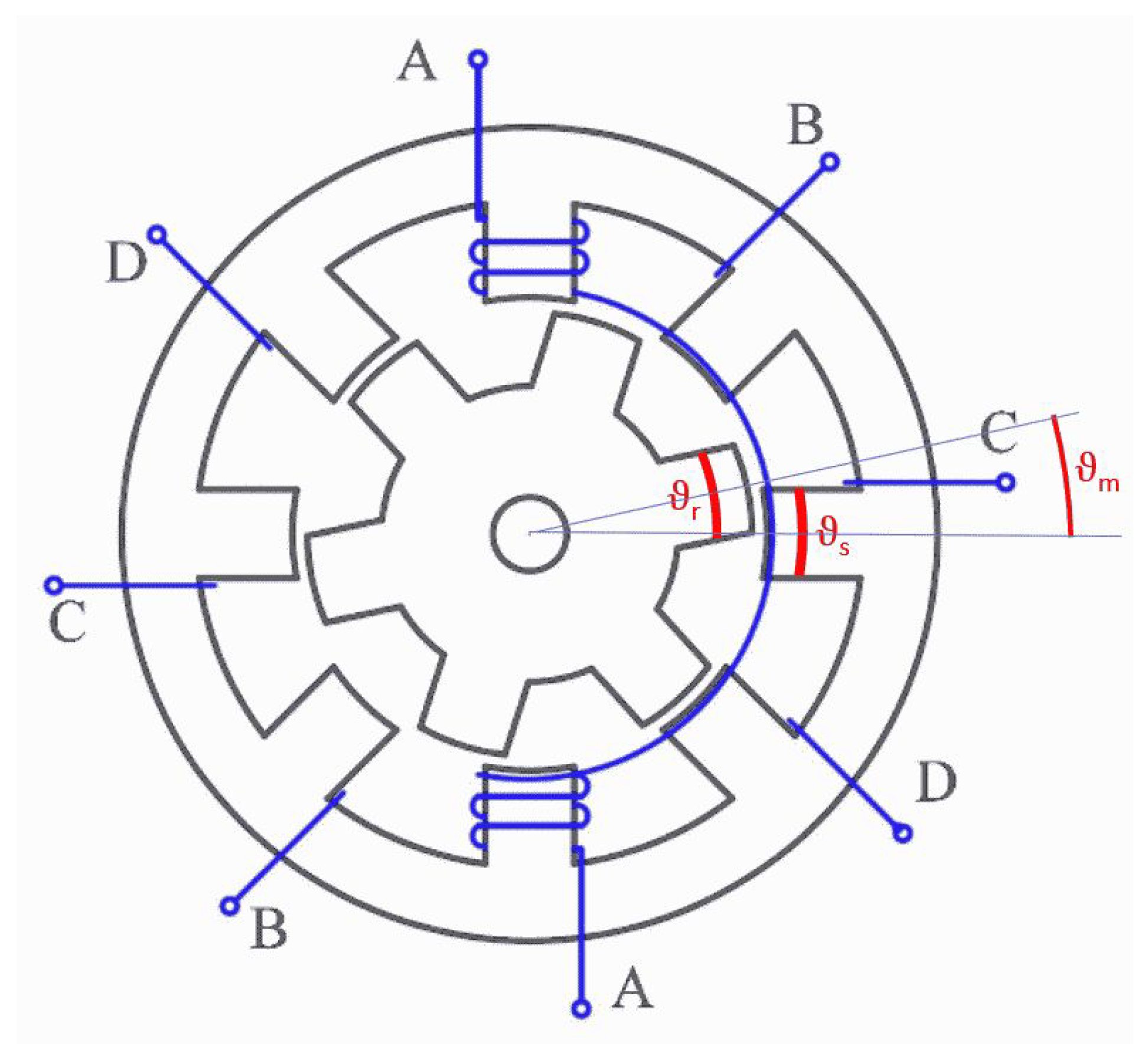
Starting from an 8/6 reference machine (see Figure 1), this work shows that, with a limited number of software simulations, it is possible to obtain six simple linear formulas which are sufficient to calculate the best angular interval for each working condition, giving good accuracy and great efficiency in real-time computation. Moreover, a very short simulation time is needed, because these formulas are able to calculate the right boundary angles for non-simulated conditions too. To achieve this aim, an ordinary linear regression technique is used, so a general expression for new angles, to start and stop supplying current to a specific phase, is obtained and the predictions are sufficiently accurate, even though the considered working condition is not simulated.

2. Working Principle and Mathematical Model of the Switched Reluctance Machine

The working principle of a switched reluctance machine is very simple: rotor poles, made of bare iron, are attracted by the magnetic field generated by stator windings: when a rotor pole is aligned with a stator one, whose windings are powered, the motor does not move anymore, because the flux density magnetic field has already found a path to close its lines with minimum effort (corresponding to the minimum air gap). Dealing with speed control, to let the machine move, the current must flow through the windings of another phase, so the rotor pole is attracted by a new stator pole while the previous phase is switched off. Since the magnetic field cannot reject induced poles as in PM brushless motors, the positive or negative signs of the phase currents have the same effect on the motor rotation direction.

The electric equation of a phase of the SRM machine is reported in (1) (it is the same for each phase), where V is the phase voltage, R is the phase resistance, i is the phase current, L is the phase inductance, ${\omega }_m$ is the mechanical rotation speed, and e is the normalized back-electromotive force. All the parameters are taken from the reference machine in [1].

Going on, the inductance expression in (2) and the back-electromotive in (3) are shown, where $\mathrm{\Phi }$ stands for the magnetic linked flux and ${\theta }_m$ for the rotor mechanical angular position. In (4), co-energy is represented, as it is computed from the inductance and phase current values. Torque is shown in (5) as the derivative of co-energy over the rotor angle (in case of constant phase current), so it strongly depends on the variation in the value of inductance, which changes according to the air gap variation and magnetic saturation.

$$V=Ri+L(i,{\theta }_m)\frac{di}{dt}+e(i,{\theta }_m)w_m$$

(1)

$$L(i,{\theta }_m)=\frac{\partial \mathrm{\Phi }(i,{\theta }_m)}{\partial i}=\frac{N^{2}A\mu }{l}$$

(2)

$$e(i,{\theta }_m)=\frac{\partial \mathrm{\Phi }(i,{\theta }_m)}{\partial {\theta }_m}$$

(3)

$$W_f={\int }_0^{i}L(i,{\theta }_m)idi$$

(4)

$$T=\frac{\partial W_f(i,{\theta }_m)}{\partial {\theta }_m}$$

(5)

By manipulation of the aforementioned equations, other formulas were obtained to adapt them to the analyzed machine. In this paper, the physical model was obtained starting from the piecewise linear model in [1], depicted in Figure 2, in order to obtain a correct theoretical description of the motor behavior. This 8/6 machine was considered appropriate for our studies because it is a standard configuration; its parameters are listed in

Table 1. Geometric parameters of the analyzed 8/6 machine.

Parameter	Symbol	Value
DC voltage	$V_{dc}$	500 V
Rated speed	$w_{rated}$	100 rad/s
Rated torque	$T_{rated}$	75 Nm
Stator pole angle	${\theta }_s$	$20.1$°
Rotor pole angle	${\theta }_r$	30°
Aligned angle	${\theta }_a$	0
Unaligned angle	${\theta }_u$	30°
Aligned inductance	$L_a$	145.9 mH
Unaligned inductance	$L_u$	9.15 mH
Saturation inductance	$L_{sat}$	2.599 mH
Saturation flux	${\mathrm{\Phi }}_{sat}$	873.6 mWb
Coefficient	K	$0.1640$

; where $V_{dc}$ is the DC Link voltage of the power converter; $w_{rated}$, $I_{rated}$, and $T_{rated}$ are the rated speed, current, and torque provided by the machine; stator angle is the angular width of a stator pole, while rotor angle is the angular width of a rotor pole; aligned angle is the rotor position when a stator and a rotor pole are aligned (usually rotor poles are larger than stator ones, so “aligned” means that their axes of symmetry are collinear), and we define it as 0 for the first phase as a reference, while unaligned angle is the rotor position when a rotor pole is exactly in the middle of two stator poles, so it is 30° for the first phase (for all the other phases, these two angles are shifted by 60°); aligned inductance is the value of the inductance at the aligned angle, while unaligned inductance is the value of the inductance at the unaligned angle; saturation inductance stands for the value of the inductance when the magnetic flux is saturated in the iron and, simultaneously, a rotor and a stator pole are aligned; saturation flux is the value of the magnetic flux where the hysteresis iron graph begins to reduce its slope; the coefficient K is an experimental value included in the model in paper [1].

Referring to Figure 2, since rotor poles are larger than stator ones, the inductance remains stable until the edges of both poles overlap (this rotor position is computed as in Equation (6)), then it linearly decreases until the poles no longer overlap (rotor position in Equation (7)) down to the value of unaligned inductance. Then, it remains constant until the rotor pole sees the edge of the following stator pole (rotor position in Equation (8)). After that, it linearly rises until the rotor and stator poles are completely overlapped (rotor position in Equation (9)). This variation repeats with a mechanical periodicity of $\frac{\pi }{3}$ in each phase.

$${\theta }_1=\frac{{\theta }_r-{\theta }_s}{2}$$

(6)

$${\theta }_2=\frac{{\theta }_r+{\theta }_s}{2}$$

(7)

$${\theta }_3=\frac{\pi }{3}-{\theta }_2$$

(8)

$${\theta }_4=\frac{\pi }{3}-{\theta }_1$$

(9)

The study of this article focuses on a control which can be suitable for all kinds of SRMs, otherwise peculiar features of the considered machine would prevent the results from being considered reliable and general. As suggested by [2], the main Fourier harmonics can be successfully used to approximate the piecewise model and calculate a more realistic model; to achieve this purpose, the curve fitting tool in MATLAB was used to compute the Fourier coefficients. This kind of approximation is used since the physical description of the magnetic flux according to Lenz’s law is not sufficient to express how the inductance varies in an SRM, since the non-zero tolerances of the manufacturing of the teeth of rotor and stator, together with the mere dispersion of the magnetic flux, cause a “rounding” of the inductance trend, which is clearly visible in all SRMs. Consequently, a piecewise linear function is not the best solution to describe this process. Even though the reliability of the model was not verified through experiments, these standard formulas are considered sufficient to prove the effectiveness of the new control strategy with the electrical simulator software PLECS.

The obtained formulas are shown below. In (10), there are some coefficients which appear in the following expressions: those in (11) and (12) (which is the derivative of (11), with a little change in the fifth harmonic coefficient to adapt it to the shape of real torque) are used to support the following ones ((13) for magnetic flux, (14) for inductance, (15) for back-electromagnetic force, and (16) for torque); the variable “x” stands for the phases (0 for phase 1, 1 for phase 2, 2 for phase 3, 3 for phase 4); the angle ${\theta }_m$ represents the mechanical rotor angle. All values depend on the phase currents and mechanical angles.

$$k_0=0.5001;k_1=0.5255;k_3=0.001;k_5=-0.0207$$

(10)

$$f_x\left({\theta }_m\right)=k_0+\sum _{i=1,3,5}{k}_{i}cos\left(6i({\theta }_m+\frac{\pi x}{4})\right)$$

(11)

$$f_x^{\prime }\left({\theta }_m\right)=-6k_{1}sin\left(6({\theta }_m+\frac{\pi x}{4})\right)-\frac{30}{4}{k}_{5}sin\left(30({\theta }_m+\frac{\pi x}{4})\right)$$

(12)

$$\mathrm{\Phi }(i,{\theta }_m)=L_{u}i+f_x\left({\theta }_m\right)({\mathrm{\Phi }}_{sat}(1-\left(e^{-Ki}\right))+(L_{sat}-L_u)i)$$

(13)

$$L(i,{\theta }_m)=L_u+f_x\left({\theta }_m\right)((L_a-L_{sat})e^{-Ki}+L_{sat}-L_u)$$

(14)

$$e(i,{\theta }_m)=f_x^{\prime }\left({\theta }_m\right)({\mathrm{\Phi }}_{sat}(1-e^{-Ki})+(L_{s}at-L_u)i)$$

(15)

$$T_x(i,{\theta }_m)=f_x^{\prime }\left({\theta }_m\right)({\mathrm{\Phi }}_{sat}i-\frac{{\mathrm{\Phi }}_{sat}}{K}(1-e^{-Ki})+\frac{i^2}{2}(L_{sat}-L_u))$$

(16)

In all of the following figures, the current is set to 50 A, but its value is not relevant, because we just want to show the typical trends. In Figure 3, phase inductances are represented as they vary with the angular position of the rotor and with the current; Figure 4 shows the evolution of the torque contribution in every phase, pointing out the corresponding intervals. It is extremely important to notice that each phase can provide torque in both directions depending on the angular position of the rotor when current flows through a specific phase. So it is possible to identify some angular intervals which will be useful to the control scheme. When the requested working condition is motor, current flows just in the phase windings which, for that instantaneous angular position, provide positive torque; otherwise, when the working condition is generator, current flows in those phases which provide negative torque.

In

Table 2. Angular intervals and their corresponding working conditions.

Phases	Motor (T > 0)	Generator (T < 0)
Phase 1	$\frac{\pi }{6}\le {\theta }_m\le \frac{\pi }{3}$	$0\le {\theta }_m\le \frac{\pi }{6}$
Phase 2	$0\le {\theta }_m\le \frac{\pi }{12}$ v $\frac{\pi }{4}\le {\theta }_m\le \frac{\pi }{3}$	$\frac{\pi }{12}\le {\theta }_m\le \frac{\pi }{4}$
Phase 3	$0\le {\theta }_m\le \frac{\pi }{6}$	$\frac{\pi }{6}\le {\theta }_m\le \frac{\pi }{3}$
Phase 4	$\frac{\pi }{12}\le {\theta }_m\le \frac{\pi }{4}$	$0\le {\theta }_m\le \frac{\pi }{12}$ v $\frac{\pi }{4}\le {\theta }_m\le \frac{\pi }{3}$

, these observations are summarized (since the machine periodicity is $\frac{\pi }{3}$, intervals are specified until this value).

3. Control Scheme

To assure the correct value of current to all windings, a standard asymmetrical converter for SRM drives was chosen for the power electronics. A PWM frequency of 20 kHz was provided to guarantee a proper supply to the phases of the machine; this value was chosen since it is quite common in most industrial applications of electric drives. Figure 5 shows the first leg of the asymmetrical power converter used to drive phase 1, and it is identical to each of the four-phase windings. $V_{DC}$ is the DC Link input voltage, $S_{i}1$ and $S1$ are the two gate control signals which drive the transistors. We refer to $S_{i}1$ as the interval signal and to $S1$ as the PWM signal. This configuration is widespread for the control of SRMs, as it is very efficient, especially when the machine works as a motor (as shown in [5], another kind of power electronics is more appropriate if the machine works mainly as a generator in order to achieve higher performance).

There are four different working modes for the asymmetrical converter: in charge mode, the current flows from the input DC voltage to the winding, as the two transistors are closed; in demagnetization mode, both switches are open, so the current passes through the two diodes, which have the function of accelerating the discharge of the phase inductance; in free-wheeling mode, just one transistor is closed and the phase machine current flows through this transistor and only a diode. In this last case, the current discharge is slower than demagnetization. In our control strategy, the charge mode and free-wheeling mode are used to regulate the current in the windings, by increasing (the former) or slowly decreasing (the latter) its value, in order to remain as stable as possible; whereas, demagnetization mode is used to lead the current to zero quickly when it is necessary to change the winding through which current is supplied.

For the sake of simplicity, the explanation of the current phase control scheme is carried out only for phase 1. For the other phases, the strategy is the same.

Figure 6 shows the current control scheme for phase 1. The inputs of this block are shown in blue, while the outputs are shown in red. $I^{*}$ is the reference current provided by the outer closed-loop speed control. ${\theta }_m$ is the input which comes from the position sensor on the rotor, but in the first block, the phase 1 activation condition takes into account the machine periodicity of $\frac{\pi }{3}$, so the residual of the division between the actual mechanical angle ${\theta }_m$ and $\frac{\pi }{3}$ is computed. $I_1$ is the sensed current of phase 1. The outputs of this scheme are $S_{i}1$, as the interval signal, and $S1$, as the PWM signal; both are used to drive the transistors on leg 1. In a traditional control scheme, the interval signals are based on angles that coincide with those indicated in Table 2. This check is made in the block “phase 1 activation condition” too. In the case of phase 1 and the motor working condition, ${\theta }_{mON-ph1}$ is $\frac{\pi }{6}$ and ${\theta }_{mOFF-ph1}$ is $\frac{\pi }{3}$. As a result, the interval signal $S_{i}1$ will be 1 if $\theta$ is between ${\theta }_{mON-ph1}$ and ${\theta }_{mOFF-ph1}$, otherwise it will be 0. This value is passed through an AND with $I^{*}$, so the reference current of phase 1 $I_1^{*}$ will be 0 if the phase is not requested to supply energy. If $S_{i}1$ is 1, $I^{*}$ coincides with $I_1^{*}$, so it is passed to the current control loop, taking the real value of current $I_1$ and calculating the duty cycle d of PWM, from where the $S1$ PWM signal is obtained.

The interval signal $S_{i}1$ will drive one of the two transistors of leg 1, while the PWM signal will drive the other one. As a consequence, when $S1$ is 1, both transistors will be closed and charge mode will be implemented, otherwise ($S_{i}1$ set to 1 and $S1$ set to 0) free-wheeling mode will be set. Finally, when $S_{i}1$ is 0, S1 will be 0 too, and demagnetization mode will occur.

It is a key point of this paper to demonstrate that the effectiveness of torque ripple reduction strongly depends on the alternation between the demagnetization and free-wheeling modes to smooth the overlap of two successive torque phases. It is relevant to point out that free-wheeling mode is not possible in the generator working condition, because of high values of the back-electromagnetic force, which slow down the current charge transient, so only charge and demagnetization modes can be used.

In Figure 7, the basic control scheme is shown: a speed feedback control has been implemented in the SRM in this article. It takes the reference $w^{*}$ from the user and sensed speed $w_r$ to provide the reference of current $I^{*}$ to each phase. Inside the block “current control phases 1, 2, 3, 4”, there are current controls, as we have already seen in Figure 6. This block produces all interval signals and PWM signals, which are inputs for the following block, “asymmetrical power converter”, that symbolizes the power electronics. The results of the control signals are currents flowing in the windings of the motor, a model of which is represented by the block “SRM“. The goal of the currents is to provide the appropriate torque, which balances the external resistant torque $T_r$, and gives the desired speed $w_r$. Phase currents are sensed and used to build feedback current control; finally, the angle ${\theta }_m$ of the rotor is measured and brought into the “phase activation condition” block of each phase.

What we have just analyzed is the basic control scheme for SRMs, but in the literature, complicated strategies have been applied to improve the efficiency and reduce the torque ripple. One of the best performing strategies is direct instantaneous torque control (DITC); see, e.g., [7].

In Figure 8, the ordinary DITC control scheme is displayed: a middle feedback loop of torque is located between the speed and current ones in order to minimize the torque ripple. This is almost identical to the previous scheme in Figure 7, but the block “PI control torque” has been added, which takes the reference of torque $T^{*}$ coming from the outer speed control loop and provides the reference current $I^{*}$ to the current controller. Obviously a torque sensor is much more expensive than position and current ones, but if an accurate torque model is calculated, that sensor is not needed. Of course, as said in the previous paragraphs, obtaining a reliable model for SRMs is very difficult, so there might be noticeable differences between real and virtual experiments on SRMs controlled by DITC. In this paper, some simulations with DITC, linked with the new proposed control strategy, will be shown at the end.

A few more observations are needed. In both kinds of controls, resistant torque $T_r$ is treated as noise, as it is not measurable, while real torque is estimated as T and calculated in DITC with Formula (16); since it fluctuates a lot because of machine reluctance, it is passed through a low-pass filter in order to obtain a more stable sensing. In our simulations, we have set the reference speed and the resistant torque, and the reference torque and current are computed by the two PI regulators (reference current $I^{*}$ is passed to a low-pass filter to obtain a better stability too). This paper focuses on the motor working condition (first quadrant), but if we wanted to design a four-quadrant control, we would have needed to consider the signs of $w^{*}$ and $T^{*}$ to understand which working condition was requested by the user and to calculate the appropriate interval signals, as shown in Figure 2. Finally, all the regulators are ordinary PI regulators, whose tuning was performed using the standard Ziegler–Nichols method.

4. Proposed Current Control

The new proposal in this article consists in reducing the angular interval of current supply for each phase of a switched reluctance machine. Figure 9 shows modifications to the current control due to the new strategy: ${\theta }_{adv}$, ${\theta }_{delay}$, and ${\theta }_{dem}$ are the new inputs of this block; the demagnetization angle and the delay angle change the angular interval of the current supply at the start of the flow, while the advance angle is used to separate free-wheeling from demagnetization. This working condition is implemented in the block “phase 1 free-wheeling condition”: when ${\theta }_m$ is between ${\theta }_{adv}$ and ${\theta }_{dem}$, only one transistor must be on, which is the one driven by $S_{i}1$, while the one driven by $S1$ must be off; as a consequence, in this condition, the output of the block is a null reference current, which leads the PWM signal to be 0 too. In this way the powering of the phase is delayed by a certain quantity, while its shutdown is anticipated (coherently with demagnetization and free-wheeling modes). The way these two values are computed will be shown in the next section.

5. Proposed Simulation Strategy

The following simulation strategy allows the angular interval which minimizes the torque ripple for each working condition to be found. The flow diagram of this strategy is shown in Figure 10. The aim of this method is to associate a finite number of couples $(w^{*},T_r)$ to a couple $({\theta }_{ON},{\theta }_{OFF})$. Considering the symmetry and periodicity of the machine, finding a new interval for each phase is not needed; so calculating an advance angle${\theta }_{adv}$ (angle corresponding to how much the switching off of a phase is anticipated) and a delay angle${\theta }_{delay}$ (angle corresponding to how much the switching on of a phase is delayed) will be sufficient. As a consequence, these new two values will be subtracted and added to those written in Table 2. In this way, it would be much more simple to apply the concept of the new angular interval to the working conditions of all four quadrants, even though our focus is on working as a motor. For the sake of simplicity, in this paper, only the results of simulations for positive speeds and torques are shown.

The simulations to find the optimal angles were performed using the basic control scheme shown in Figure 7 and Figure 9, as understanding discontinuities between two subsequent phases is easier to obtain than in the DITC control scheme in Figure 8. The steps to follow for the strategy are the following:

• Dataset creation: create a random table with values of speed and torque in the acceptable range of working conditions. Some libraries of Python make this task very easy. To generate them, a Gaussian distribution is recommended, since it will give as output fewer working conditions at the boundaries of the assigned range and more in the middle (more frequent working conditions). In this paper, only 60 couples of $(w^{*},T_r)$ are taken, and some of them are used to compute the accuracy of the model, so less than 60 are actually needed to compute the desired formula. The more there are, the more accurate the model will be. The fewer there are, the lower the simulation time will be.
• Start simulation: start the simulation (in this paper all the simulations are performed with the electrical software PLECS) of a working condition taking into account two values: the time needed by the system to reach a steady-state operating condition (for this machine, stability is reached at about 0.06 s, so 0.1 is a good confidence margin); the reference current ($I^{*}$) is taken when a steady-state operation condition is reached ($t=0.1$ s). After that time, variations to the intervals will be applied. $I^{*}$ is needed because it is strongly correlated with the resistant torque $T_r$, which we cannot measure (otherwise an expensive torque sensor will be needed), so its value will be used in the final formulas of our linear regression model. Remember that is very important to take note of the value of $I^{*}$ after the variations in the intervals, not before: the control system reacts to the reduction in angular intervals by increasing the reference current $I^{*}$, so, if we took the value before the angular interval restriction, the regression model would be trained on the wrong data. This behavior will become more clear in the simulation section. It is recommended to test each working condition for at least 1 s (with a low-cost personal computer of 16 GB RAM, 1 s of PLECS simulation lasts for about 10–15 “real” seconds), so a lot of possible angle values can be tested within 0.9 s, and they can be found with more accuracy.
• Advance angle definition: during these simulations, it’s been noticed that there is an angular position where, for a fixed value of current, the torque begins to slow down; in order to find an appropriate compromise between efficiency and continuity of torque supply, each phase should be switched off around this point. This can be found easily by simulation, and it corresponds (in most cases) to an advance angle${\theta }_{adv}$ of about 42% of the entire size of the interval (it may be a bit lower for high torques and a little higher for low torques or low speeds), but if it does not change in a noticeable way, the effects on the torque ripple will be insignificant. PLECS can automate this step by testing some angle values and reading the one which minimizes the torque ripple for that fixed couple speed–resistant torque. It is recommended to test each condition with some advance angles with a step of 0.008 rad (higher for a faster simulation, lower for a better accuracy).
• Delay angle definition: to smooth the transition between the ongoing phase and the incoming one, a delay angle${\theta }_{del}$ has to be applied to the powering of each phase. In this part of the simulation, this value is changed until the condition of minimum torque is satisfied. Even though this step could seem very long in terms of time, actually the acceptable results cover quite a large range of values, as a little change in ${\theta }_{delay}$ does not change the torque ripple significantly. In Figure 11, a typical situation that must be realized is displayed: notice the trend in the resultant torque T between two different “valleys”, which corresponds to those intervals when torque depends on the contribution of a single winding, while “valleys” refers to the transition between two consecutive phases. It is recommended to test each condition with some delay angles with a step of 0.0014 rad (higher for a faster simulation, lower for a better accuracy).
• Free wheeling and demagnetization: when a phase is switched off, it enters free-wheeling mode to soften the transition with the incoming phase. Taking another advance angle for demagnetization ${\theta }_{dem}$ is strongly suggested. In most cases, this angle is calculated by dividing the ${\theta }_{adv}$ by 2 (for this kind of SRM machine). For low speeds and low torques, it can also be fixed to 4, but the overall shape of the torque trend does not change considerably. At this step, the phase torques should look like in Figure 12.
• Dataset completion: through repeating steps 2–5 for all working conditions, the final dataset is obtained. It is important to store the reference speed, reference current (as already said, taken after the change in the angular interval), the delay angle ${\theta }_{delay}$, and the advance angle ${\theta }_{adv}$. It is recommended to find ${\theta }_{adv}$ first, then fix it, and finally start the simulation to search for the best ${\theta }_{delay}$.

6. Linear Regression: Model Calculation

This paragraph shows how a simple linear formula can be computed to obtain the advance angle ${\theta }_{advance}$ and delay angle${\theta }_{delay}$ for each possible combination of speed and torque. In this way, in a real-time application, the SRM will be able to change its parameters quickly (angular intervals of current supply) and adapt itself. To achieve this purpose, basic data analysis techniques were used. Python offers many libraries with optimized calculations of models, given some features, to predict a target variable. By looking at the correlation matrix displayed in

Table 3. Correlation matrix between main features.

Parameters	Reference Speed	Torque Resistance	Theta off Advance	Current Reference	Theta on Delay
Reference Speed	$1.00$	$-0.10$	$-0.15$	$-0.07$	$-0.87$
Torque resistance	$-0.10$	$1.00$	$-0.68$	$1.00$	$0.07$
Theta_off advance	$-0.15$	$-0.68$	$1.00$	$-0.67$	$-0.02$
Current reference	$-0.07$	$1.00$	$-0.97$	$-1.00$	$0.04$
Theta_on delay	$-0.87$	$0.07$	$-0.02$	$0.04$	$1.00$

, we see that our main features are reference speed $w^{*}$ and reference current $I^{*}$ (the correlation between reference current and resistant torque $T_r$ is 1, so we can use it to replace resistant torque $T_r$, which cannot be measured), in fact the reference current has high values of correlation with both ${\theta }_{adv}$ and ${\theta }_{delay}$. Many models can be used, and modern techniques may achieve very accurate predictions. In this paper, linear regression models are used for two main reasons: first, they are simple, in fact they are just linear formulas with two weights (numbers which multiply both features) and a known term; second, they do not occupy so much memory space, so they do not require a long time to execute calculations; and finally, the motor can easily adapt new angular intervals to variations in real-time working conditions.

The library ‘sklearn’ was sufficient for the purpose of automatically making these calculations, but care must be taken with the parameter ‘test size’ to avoid overfitting: the model might adapt itself too much on the training data instead of obtaining the general trend of the targets. Therefore, some examples from the dataset were used to train the model, the remaining ones to evaluate it. To make the model more accurate (since it hides a non-linearity), the dataset was split into three groups by the value of $I^{*}$ (less than 11 A, more than 32 A, and middle values), so we obtained three linear formulas to compute the advance angle${\theta }_{adv}$ and three for the delay angle${\theta }_{delay}$. The introduction of $I^{*}$-splitting indicates the system’s non-linearity, so linear calculations are just an approximation. Below, all formulas of the models are shown, while relevant statistics are presented in

Table 4. Statistics of linear regression model for advance angle.

Groups Ranges	Total Samples	Train Samples	Test Samples	Train RMSE	Test RMSE
$I^{*}\le 11$	10	6	4	$0.001658$	$0.003287$
$11<I^{*}<32$	30	27	3	$0.004057$	$0.003078$
$I^{*}\ge 32$	20	13	7	$0.002102$	$0.002593$

and

Table 5. Statistics of linear regression model for delay angle.

Groups Ranges	Total Samples	Train Samples	Test Samples	Train RMSE	Test RMSE
$I^{*}\le 11$	10	6	4	$0.001811$	$0.002877$
$11<I^{*}<32$	30	28	2	$0.004574$	$0.003823$
$I^{*}\ge 32$	20	16	4	$0.003627$	$0.002334$

, expressed in terms of the root mean square error (RMSE; useful for defining how far from the simulated value a prediction is on average) for both the train and test sets and for the three groups.

$$(I^{*}\le 11){\theta }_{adv}=-1.97·{10}^{-4}{w}^{*}+1.4·{10}^{-3}{I}^{*}+0.2417$$

(17)

$$(I^{*}\ge 32){\theta }_{adv}=-6.7·{10}^{-4}{w}^{*}-2.2·{10}^{-4}{I}^{*}+0.2422$$

(18)

$$\left(I^{*}ϵ(11,32)\right){\theta }_{adv}=-3.19·{10}^{-4}{w}^{*}-1.33·{10}^{-3}{I}^{*}+0.2577$$

(19)

$$(I^{*}\le 11){\theta }_{delay}=1.00·{10}^{-4}{w}^{*}+4.96·{10}^{-4}{I}^{*}+0.0247$$

(20)

$$(I^{*}\ge 32){\theta }_{delay}=1.4·{10}^{-4}{w}^{*}+8.1·{10}^{-4}{I}^{*}+3.9·{10}^{-4}$$

(21)

$$\left(I^{*}ϵ(11,32)\right){\theta }_{delay}=1.8·{10}^{-4}{w}^{*}+2.8·{10}^{-4}{I}^{*}+0.0169$$

(22)

Note two aspects: the splitting into the train and test sets had the one aim of computing the RMSE on both datasets and justifying the effectiveness of the model, so we need less than 60 simulations to have reliable control; these models are obviously approximated, but the accuracy is sufficient for our purpose, as too much precision is not needed (as said before, a certain range of values of angles is acceptable with no significant variation in the torque ripple).

In the case of the generator working condition, the delay angle ${\theta }_{del}$ does not vary, instead the advance angle ${\theta }_{adv}$ must be divided by 2 (or eventually by 4) because it coincides with ${\theta }_{dem}$ (as already explained, there is no free-wheeling mode if SRM works as a generator if we use the asymmetrical power converter).

To better explain this kind of computation, an example is given. If the reference speed is set to $w^{*}=50$ rad/s and the resistant torque is set to $Tr=10$ Nm (the reference current obtained by the outer current control loop is near 10 A), the angles of supply interval obtained using the equations displayed are the following: ${\theta }_{del}=0.03466$ rad, ${\theta }_{adv}=0.233325$ rad, and ${\theta }_{dem}=0.013864$ rad.

$$(I^{*}\le 11AND{w}^{*}\le 12){\theta }_{dem}=\frac{{\theta }_{adv}}{4}$$

(23)

$$(I^{*}\ge 11OR{w}^{*}\ge 12){\theta }_{dem}=\frac{{\theta }_{adv}}{2.5}$$

(24)

7. Simulations and Final Results

In these final paragraphs, extensive simulations in the PLECS environment are carried out to prove the effectiveness and reliability of this strategy.

Figure 13 and Figure 14 show the new control strategies, obtained by the previous standard controls, basic and DITC, with the addition of the block “angular interval calculation”. This block takes the reference speed $w^{*}$ and the reference current $I^{*}$ as inputs and calculates the angles as outputs; then, they become inputs of all phases of the current controls. These schemes were used to evaluate the performance of the proposed strategy applied to the standard controls.

In the following figures, the evolution of the main quantities is shown (the basic and DITC trends are similar, even though they have different values) for a sample working condition of reference speed $w^{*}=80$ rad/s and a resistant torque $Tr=30$ Nm. The angles of supply interval obtained using the equations shown in the previous section are the following: ${\theta }_{del}=0.0337$ rad, ${\theta }_{adv}=0.23085$ rad, and ${\theta }_{dem}=0.09234$ rad.

The simulation was set up in this way: the reference speed was given at the beginning of the simulation (at t = 0.0 s), while resistant torque was applied at t = 0.1 s. This was to point out the reactivity of the control to the noise $T_r$. The machine reaches the regime condition at about 0.2 s, at which point the formulas are used to compute the new angular intervals. At this point, the reference current increases and the torque ripple decreases.

In Figure 15, Figure 16, Figure 17 and Figure 18, the trends in the speed, reference current, phase currents, and total torque are presented. At the time the new angular interval is introduced (t = 0.2 s), fluctuations decrease visibly, demonstrating the effectiveness of the strategy. In Figure 19 and Figure 20, zoomed trends of the current and torque are depicted. It is evident how the control is easily adapting to the new angular interval, and fluctuations remain in a limited range even though the main phase which provides the current is changing. In Figure 21 and Figure 22, trends in the phase currents and torque are shown for the basic control strategy. It is noticeable that, after the reduction in the angular interval, the phase currents have a small overlap between the previous one and the next one. Since torque is provided by two different phases for a small range of angles, the result of the reduction in the torque ripple is evident.

Table 6. Simulation results of new basic control scheme compared with traditional basic control.

Speed (rad/s)	Resistant Torque (Nm)	RMS Current on DC Link (A)	RMS Phase Currents (A)	Torque Ripple (Nm)	Reduction of RMS Current on DC Link	Reduction of RMS Phase Currents	Reduction of Torque Ripple
15	5	$1.19$	$3.00$	$2.31$	$24.68\%$	$25.00\%$	$14.13\%$
17	45	$6.90$	$13.60$	$12.93$	$14.50\%$	$17.58\%$	$40.44\%$
40	75	$16.00$	$21.80$	$14.75$	$16.10\%$	$5.63\%$	$59.13\%$
60	10	$3.89$	$4.93$	$3.06$	$32.47\%$	$13.51\%$	$56.47\%$
80	30	$10.20$	$9.80$	$8.78$	$24.11\%$	$14.78\%$	$53.72\%$
110	35	$13.41$	$11.25$	$8.17$	$23.46\%$	$15.41\%$	$83.08\%$
130	8	$5.24$	$4.80$	$3.52$	$35.71\%$	$19.33\%$	$56.00\%$

,

Table 7. Simulation results of new basic control scheme compared with traditional DITC control.

Speed (rad/s)	Resistant Torque (Nm)	RMS Current on DC Link (A)	RMS Phase Currents (A)	Torque Ripple (Nm)	Reduction of RMS Current on DC Link	Reduction of RMS Phase Currents	Reduction of Torque Ripple
15	5	$1.19$	$3.00$	$2.31$	$30.00\%$	$23.08\%$	$-65.00\%$
17	45	$6.90$	$13.60$	$12.93$	$15.85\%$	$17.07\%$	$79.58\%$
40	75	$16.00$	$21.80$	$14.75$	$15.34\%$	$6.84\%$	$-20.51\%$
60	10	$3.89$	$4.93$	$3.06$	$34.84\%$	$13.51\%$	$-6.62\%$
80	30	$10.20$	$9.80$	$8.78$	$24.89\%$	$15.52\%$	$-38.05\%$
110	35	$13.41$	$11.25$	$8.17$	$23.11\%$	$16.67\%$	$0.73\%$
130	8	$5.24$	$4.80$	$3.52$	$25.78\%$	$19.33\%$	$21.08\%$

and

Table 8. Simulation results of new DITC control scheme compared with traditional DITC control.

Speed (rad/s)	Resistant Torque (Nm)	RMS Current on DC Link (A)	RMS Phase Currents (A)	Torque Ripple (Nm)	Reduction of RMS Current on DC Link	Reduction of RMS Phase Currents	Reduction of Torque Ripple
15	5	$1.18$	$3.03$	$1.36$	$30.59\%$	$22.31\%$	$2.86\%$
17	45	$6.81$	$13.60$	$5.86$	$16.95\%$	$17.07\%$	$18.61\%$
40	75	$15.91$	$22.5$	$11.1$	$15.82\%$	$3.85\%$	$9.31\%$
60	10	$3.90$	$4.90$	$1.43$	$34.67\%$	$14.04\%$	$50.17\%$
80	30	$10.17$	$9.98$	$4.16$	$2.58\%$	$13.97\%$	$34.52\%$
110	35	$13.23$	$11.22$	$4.06$	$24.14\%$	$16.89\%$	$50.63\%$
130	8	$5.14$	$4.7$	$2.2$	$37.01\%$	$21.01\%$	$50.67\%$

show the performance of the proposed strategy (based on a reduction in the angular interval of the current supply) in comparison with the traditional basic control scheme and standard DITC control, which uses an exact estimate of the machine torque (in actual applications this is not possible).

The tabulated values refer to steady-state conditions, using the same reference mechanical speeds and resistant torques for all the comparisons.

The performance indices are as follows: the torque ripple, computed as the difference between the maximum and minimum values of instantaneous torque; and the RMS phase current. Table 6 shows the values of these quantities with the new basic control, adopting the proposed strategy. In the right part of the table, it is possible to see the percentage reduction in these quantities with respect to the basic control. Table 7 has the same structure and presents a comparison of the new basic control with a (ideal) standard DITC. In Table 8, the proposed strategy was applied to the standard DITC. When there is a—before the percentage, it means that the value has become worse.

As shown in the tables, focusing on the “reduction of torque ripple” column, the value is positive in each working condition. Improvements in torque ripple minimization are achieved using the new simulation strategy.

For all values of reference speed and resistant torque, there are noticeable improvements in terms of the RMS phase currents, too. This means that minimizing the torque ripple not only helps the bearings work, but also reduces the Joule effect and heat losses, as this effect is related to the RMS value of the currents. Therefore, the efficiency of the machine is increased too. For some working conditions, a reduction in the supply interval, without using DITC, gives values of torque ripple similar to the standard DITC. If associated with DITC, the proposed strategy reduces the torque ripple even more.

8. Conclusions

This article proposes a new simulation strategy to find the angular intervals that minimize the torque ripple in each admitted working condition of a four-phase 8/6 SRM. After creating a dataset with advance and delay angles for a small amount of simulations, a linear regression model was used to find formulas which allowed the angles to be computed in real-time working conditions, so storage of the entire dataset in the microcontroller is not needed. This reduction in the intervals of current supply, added to the traditional control scheme and alternation of demagnetization and free-wheeling modes, greatly improves the machine efficiency, reducing the torque ripple and RMS phase currents. Finding new intervals and managing the currents with DITC is the key to making switched reluctance machines more competitive on the global market. Finally, as no constraints on machine geometry were applied, each advanced control scheme can be coupled with the proposed reduction in the angular interval.

9. Future Developments

This paper has proposed a simple methodology to maximize the performance of a switched reluctance machine drive. Of course, the work has not finished yet. Firstly, the DITC control itself can be optimized to favor a higher overlap between two successive torque phases, so the “hole” of erogated torque can be prevented by reducing ${\theta }_{delay}$ in dataset-building simulations. Secondly, the predictions can be improved: more accurate techniques, such as regression trees or polynomial formulas, can be used. Lastly, the robustness of the entire system must be guaranteed according to the tolerances of the machine’s parameters, especially electrical ones: the simulations and the linear regression model are not based on resistance or inductance values, but only on the length of the stator and rotor teeth (since they directly affect the angular interval to supply current). Nevertheless, if simulations are performed on a motor in a certain lot, another motor of the same lot (so with the same boundary angles calculation) could show higher torque ripple values because of electric parameter tolerances. Variations in phase resistance do not imply a susceptible rise in the torque ripple, on the contrary, a phase inductance variation (due to manufacturing and working temperature) can determine a significant variation in the instantaneous and mean torque.