1. Introduction
Currently, many large oilfields across the world have reached the later stages of oil and gas production and have high water contents. In order to establish the distribution laws of residual underground oil in reservoirs and further enhance oil recovery, petroleum geologists need to understand various parameters and their distributions within oil reservoirs as much as possible. For this, 3D geomodels can help to reveal the real characteristics of underground oil reservoirs and provide reliable geological understanding for oilfield development [
1], well planning, and program adjustment so as to increase the benefits for oil exploration. The most critical and basic method for understanding oil and gas reservoirs is to describe the reservoirs in detail by creating quantitative 3D geological models, which can supply direct technical guidelines for oil and gas field development and production; 3D geological models include facies models and property models (porosity, permeability, water/oil saturation, etc.).
Sedimentary facies control the macroscopic heterogeneity of reservoirs, which in turn determines the thickness, geometry, variation rules, and physical characteristics of oil reservoirs. Due to the decisive role played by facies in reservoir quality, there could be a combination of one or more diagenetic facies processes that affect the reservoir properties, which reflects current reservoir conditions. Therefore, facies-controlled geomodeling is generally used for fine reservoir descriptions as it offers higher accuracy than traditional one-step geomodeling, i.e., it uses geological data interpolation between wells to create 3D models based only on sample well data. The study of sedimentary facies in fine reservoir descriptions takes sedimentary systems and facies zones into account, but more importantly, so does the study of sedimentary microfacies.
To evaluate the three-dimensional spatial heterogeneity and fluid properties of reservoirs, it is necessary to create property models. Effective thickness, porosity, permeability, and fluid saturation are important reservoir evaluation parameters, so reservoir property models often include porosity models, permeability models, and water saturation models. However, due to the effect of the strong heterogeneity of physical and fluid property distributions underground, conventional deterministic geomodeling that interpolates a small number of observations cannot determine the true spatial changes in the properties. This is because, on the one hand, the spatial distributions of properties in reservoirs could be stochastic, while on the other hand, the distributions of properties are controlled by sandy reservoir units in braided river environments, which are characterized by regionalized variables. Therefore, geostatistics and facies-controlled stochastic simulation methods are the best choice for quantitatively describing the spatial distributions of properties in reservoir rocks [
2]. In terms of reservoir geomodeling (porosity, permeability, water saturation, etc.), traditional 3D geomodeling mainly involves a “one-stage modeling” method, which uses interwell data interpolation that is directly based on limited sample well data. This method is relatively simple but may not always be relevant because it is mainly suitable for geomodeling single facies or layer-cake structure geobodies. In some cases, reservoir properties have the same statistical distributions; however, reservoirs with multiple facies or complex architectures, such as split-board-like or labyrinth-like structures, reservoir properties can differ significantly between different facies, even within small regions. In fact, there are very few reservoirs with unique facies, especially in continental braided rivers and delta front deposition environments.
In view of the above problems, “facies-controlled geomodeling” or “two-stage geomodeling” methods are more suitable for real cases. Firstly, structural reservoir models and large facies frameworks must be created. Then, according to the quantitative distribution statistics, microfacies models can be created, and interwell data interpolation based on stochastic property geomodeling can be constrained by different facies. In this study, thin interbeds were one of the main causes of the oil reservoir heterogeneity, fluid movement barrier, and residual oil distribution in the middle to late stages of oilfield development and production, especially in thick-bottom water–oil reservoirs that rely on natural energy for production. The 3D distributions of thin interbeds seriously affect development effects in very large oil and gas reservoirs. Therefore, we employed an integrated geomodeling method using hierarchical mindset and embedded multipoint simulation. The primary objectives of this study were to develop a more accurate geomodeling method for braided river delta reservoirs and establish a theoretical understanding of continental braided river deposition environments, similar to the Triassic T2a1 formation in the Tarim Basin.
2. Geological Settings
The Tarim Basin has been developing from a foreland basin since the Triassic period [
3]. The Tahe Oilfield B9 area is located in the Akkol salient of the Xayar uplift in the northern part of the Tarim Basin (
Figure 1). The oil reservoir is in the Lower Triassic T
2a formation and is controlled by a structural anticline, which is in a sandstone reservoir with a low-amplitude faulted anticline and a very large volume of bottom water. The oil reservoir is mainly a natural water driving oilfield with over 20 years of development history. The T
2a formation has been divided into four sections, with the lower to upper sections being called T
2a
1, T
2a
2, T
2a
3, and T
2a
4. T
2a
1 is in conformity contact with the underlying T
1k Ketur formation and is mainly a light green to gray fine sandstone with gray conglomerated sandstone or dark gray mudstone. Only the upper section of T
2a
1 is an oil reservoir, which has a maximum thickness of about 150 m and multiple interbeds. However, the total effective reservoir thickness is only about 20 m, and there are many muddy or calcareous interbeds, with a water to oil volume ratio of more than 100. T
2a
1 has several sandy layers, and the target sandy layer is located in the upper section T
2a
1-1, which can be further divided into four rhythm sections that are separated by interbeds, with the upper to lower rhythm sections being called T
2a
1-1-1, T
2a
1-1-2, T
2a
1-1-3, and T
2a
1-1-4 (
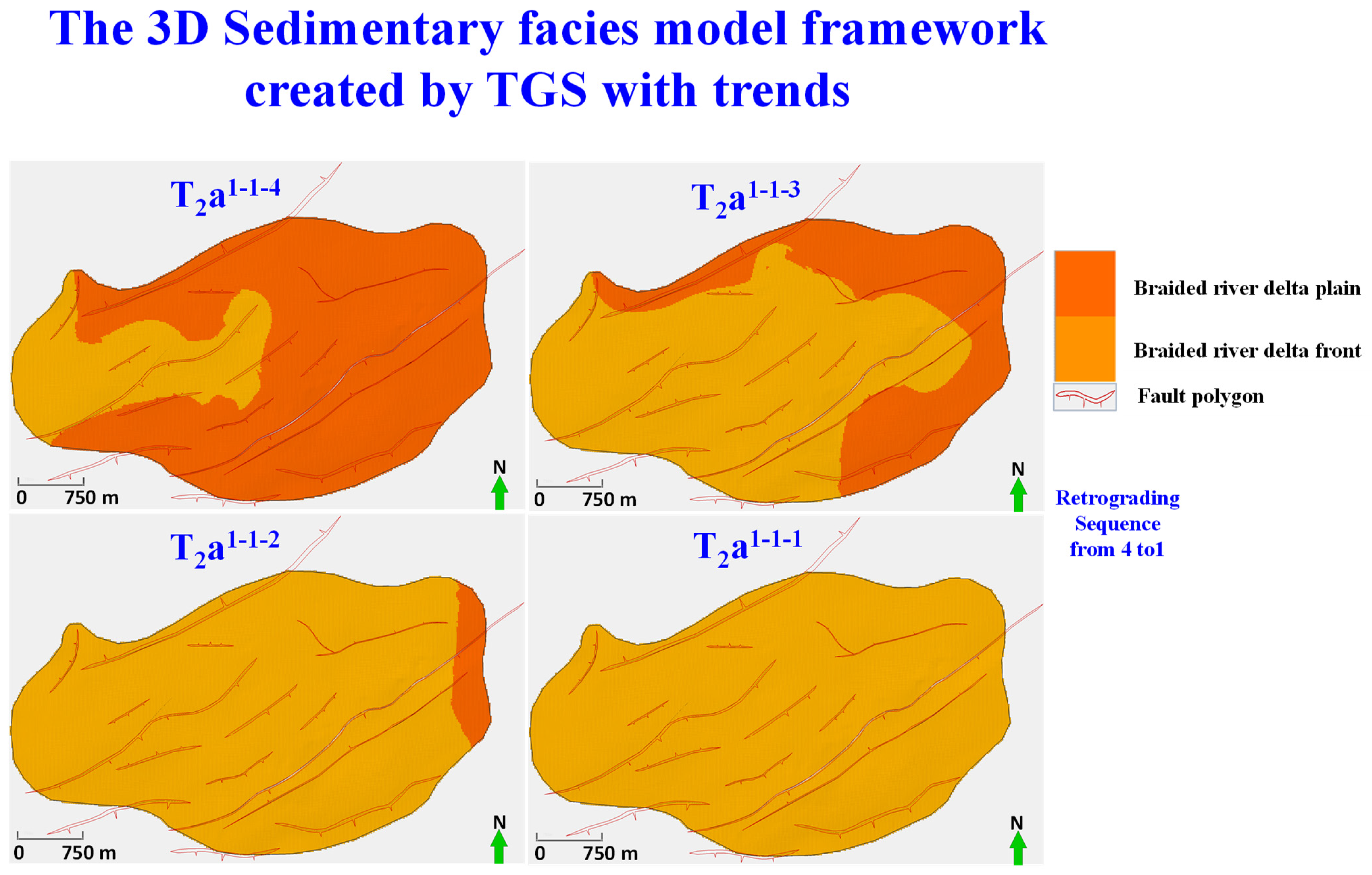
Table 1). The target sandy reservoir is deposited in a braided river delta plain and braided river delta front. A braided river delta plain retrogradation process can be observed in the deposition history from T
2a
1-1-4 to T
2a
1-1-1 (
Figure 2), and this retrogradation process was the main cause for the development of interbeds in the target sandy layer. According to the sedimentary evolution history described in previous research [
4], the deposition environment transferred from a delta plain to a delta front while the water was deepening, so the overwater distributary channel disappeared completely during the T
2a
1-1-1 deposition period. A mouth bar developed well into the later part of the period, but natural channel bars only developed in some limited areas [
5].
The Tahe Oilfield B9 area is located in a low-amplitude faulted anticline trap [
7], and the long axis of the anticline is in the northeast direction. The southern wing of the anticline is cut by a northeast azimuth normal fault, so the B9 area is divided into two asymmetric areas from north to south. The main reservoir is in the northern block, which occupies almost three quarters of the total B9 area. The northern trap closure area is about 8 km
2, with a maximum depth of −3643 m, while the southern trap closure area is 2.22 km
2, with a maximum depth of −3667 m (
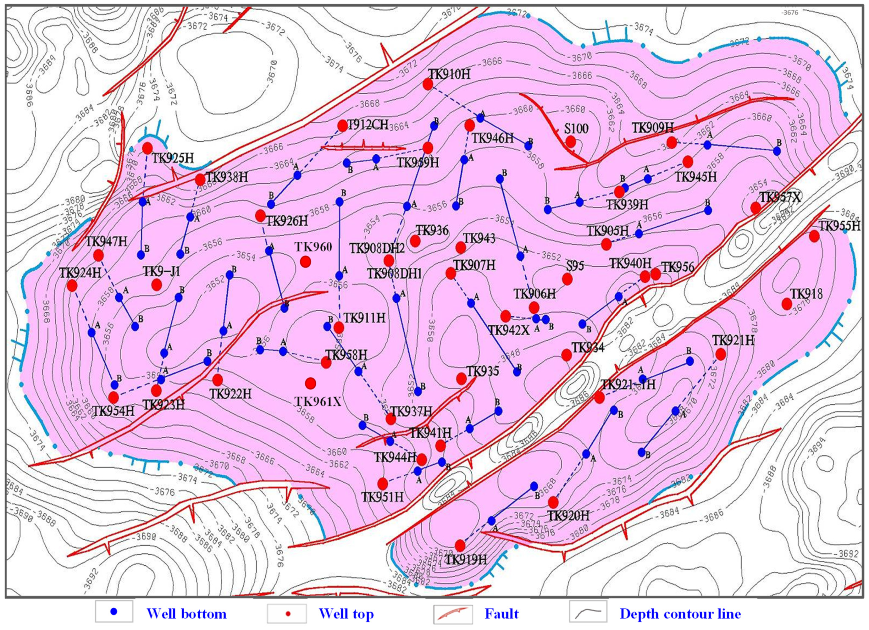
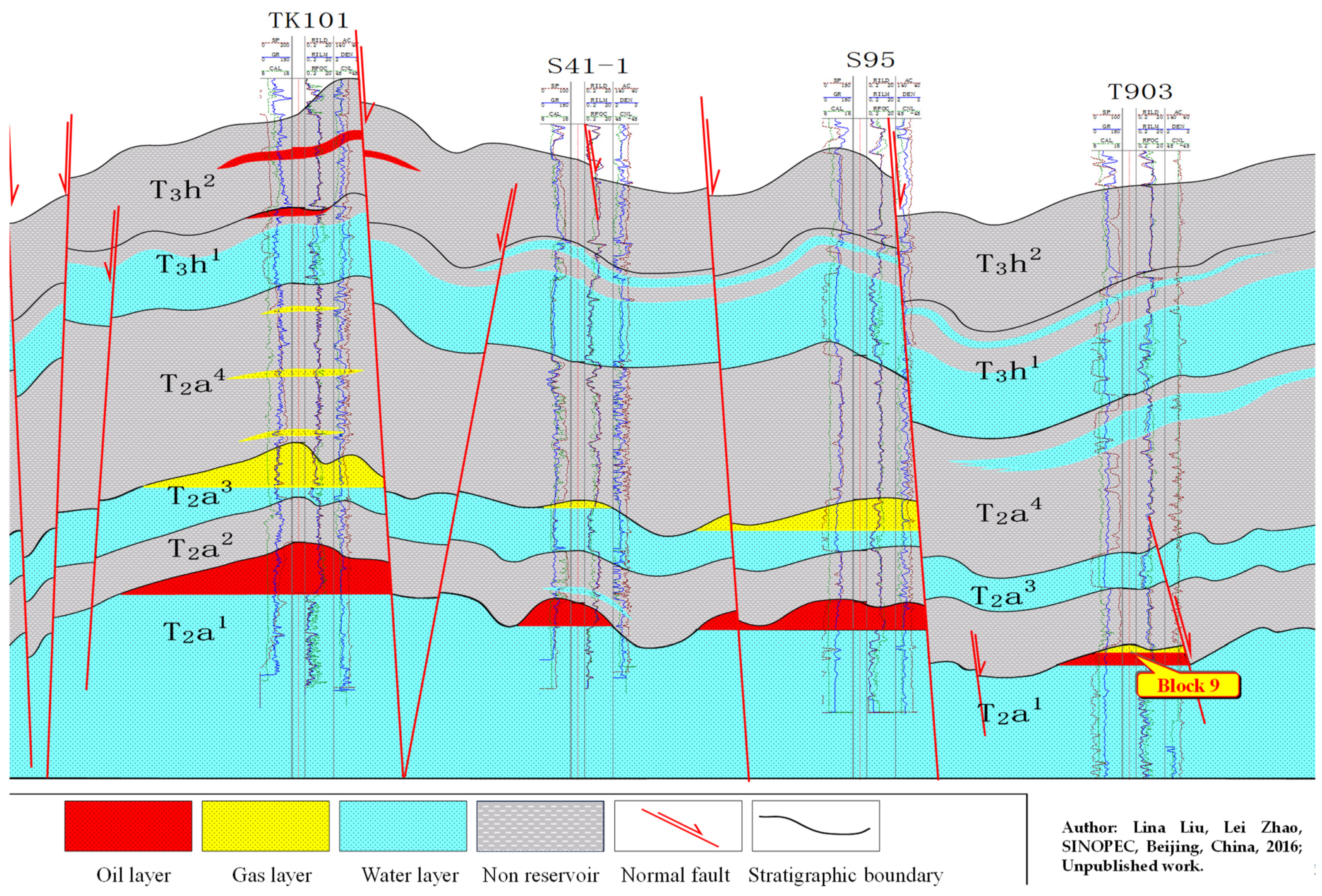
Figure 3). From the well section profile, two sets of strike-slip faults can be observed in the south, and a differential subsidence can be seen in the formation in the north of the B9 area (
Figure 4). Therefore, the anticline formed in the middle area and the northern fault are relatively more developed, making the anticline top point closer to the southern fault. These two sets of strike-slip faults control the transfer of oil and gas. Oil and gas mainly migrate upward along the northern fault, so the strike-slip faults have affected the oil and gas distributions over the course of the formation’s development. The seismic profile also provides some evidence for this conclusion [
8].
The Tahe Oilfield B9 area started to produce oil in 2002. The main well patterns are vertical wells and horizonal wells. The oilfield has now reached the late stages of oil and gas production and has a high water content. However, oil recovery is only about 25% as the complicated underground geological conditions in the B9 area make it difficult to access residual oil. Although the reservoir has medium–high porosity and high permeability in the target layers, oil development and production still face many challenges that commonly occur in continental delta deposition environments. In this study, we aimed to clarify the root causes of the following challenges:
The interbeds in this very large thick sandstone reservoir are difficult to identify and characterize;
The motion laws of the strong basal ground water and the distribution laws of the residual oil are controlled by complicated geological characteristics;
There are many wells that have high water saturation and very low oil production, so development governance is difficult without accurate 3D geomodels.
This integrated study of the lower Triassic T2a1 formation in the Tahe Oilfield B9 area, Tarim Basin, firstly confirmed the main types of sedimentary subfacies, including braided river delta plains and braided river delta fronts, and that the microfacies were overwater distributary channels, channel bars, underwater distributary channels, and mouth bars. The sedimentary evolution analysis showed that the T2a1 formation was deposited in a delta plain retrogradation environment as the base level of the water was rising.
3. Method
Facies modeling is a preliminary step in reservoir modeling workflows and is vital for evaluating property distributions that have degrees of influence on the relevant attributes, such as porosity, permeability, and water/oil saturation, which can be correlated and biased to the facies. Several types of geostatistical approaches are commonly used to allocate facies into geocellular grids, from cell-based two-point statistics to advanced multipoint statistics (MPS) algorithms. Most of the cell- and object-based simulation techniques applied in facies modeling depend on variogram models or facies geometry (such as size, orientation, and shape) when object modeling is used and are controlled by the original well data in the approximation of reservoir heterogeneity and facies geometry. To establish accurate property distributions, the MPS algorithm is used for facies propagation, in which training images and other soft probabilities guide the facies propagation [
9,
10,
11,
12,
13]. As MPS algorithms require training image grids to define relationships between individual facies, modern analogs obtained from Google Earth can be used.
We obtained all of the necessary data for this study thanks to support from the Tahe Oilfield B9 owners, which allowed us to research the identified challenges based on a subsurface dataset for the B9 area. At the same time, the subsurface dataset needed to be transformed into the specific data format that could be imported into geomodeling software. The necessary dataset included drilling data, well log data, geological stratigraphy data, outcrop geological observations, seismic interpretations, laboratory core analysis, laboratory testing data, etc.
Our proposed integrated workflow is shown in
Figure 5, with the key steps presented as the process outcomes. We first created a fine 3D structural geomodel of the study area with a grid size of 15 m × 15 m × 0.15 m and a total grid number of 27,382,000; however, the structural geomodeling was not the key step in this study, and a 3D sedimentary facies model framework was created within the structural geomodel using the MPS method to create the microfacies that were embedded into the facies model framework. Specifically, according to a well-known zonation law for the sedimentary facies in the study area, a truncated Gaussian with trends method was used to build the first-level model for the braided river delta plain and the braided river delta front. These two first-level facies were the background facies. Then, the MPS method was used to build second-level models for the four microfacies, which were an overwater distributary channel with a channel bar and an underwater distributary channel with a mouth bar. Meanwhile, the overwater distributary channel constrains the range of the channel bar, and the underwater distributary channel constrains the range of the mouth bar.
In the second step, two geostatistics simulation methods were used separately to create the 3D interbed models. The input interbed distribution data were the key in this step as the interbed distributions were determined using the well correlation results and the resistivity inversion results from horizontal wells. Object modeling and sequential indicator simulation methods were used for the 3D interbed geomodeling. The interbeds were identified as muddy interbeds and calcareous interbeds. An optimized interbed geomodel was selected from 30 stochastic realizations, and data from 32 horizontal wells were used to constrain the simulation process so as to visualize the spatial combinations of thin interbeds in the subsurface. Then, the final interbed model was optimized and selected based on the reservoir simulation results. We then combined the 3D sedimentary facies model and the 3D interbed model together to create a comprehensive facies model, which was a sedimentary-facies-plus-lithofacies model. The next step involved the property modeling, which was controlled by the comprehensive facies model. A porosity model was also simulated using separated stratigraphy and individual microfacies, which were controlled by the Gaussian random function. This formed the basis for other property models, which were validated using the laboratory core analysis and well testing results.
3.1. Sedimentary Facies Modeling
According to previous research, the sedimentary facies in the study area present a clear zonation (
Figure 2). The boundary between the braided delta plain and the braided river delta front developed during the retrogradation process of the delta plain. From the facies control perspective, different geobodies have different sizes, shapes, and features within the zonation, so we needed to use the hierarchical mindset for the facies modeling [
14,
15], i.e., the facies modeling was carried out in several levels based on the scale of the geobodies. In this study, the sedimentary subfacies, including the braided river delta plain and braided river delta front, were considered as the level 1 facies framework, and the four microfacies were also considered as the level 2 facies framework. The scales of the overwater distributary channels and underwater distributary channels across the whole study area were the same, and the channel bars were only located in the overwater distributary channel areas, while the mouth bars were only located in the underwater distributary channels. The mouth bars and channel bars were similar in shape, size, and orientation Therefore, our study considered the overwater distributary channels and underwater distributary channels within the same facies framework, which were constrained by the large facies framework. In the microfacies modeling process, the channel bar modeling was controlled by the overwater distributary channels, and the mouth bar modeling was controlled by the underwater distributary channels in the MPS simulations [
16]. This geomodeling method is known as the hierarchical mindset for modeling approach, which is widely used for complicated facies modeling.
This study used the truncated Gaussian simulation (TGS) with trends method to create the sedimentary facies model framework. The TGS with trends is a pixel-based algorithm and a fast-modeling technique for discrete properties (facies model), in which facies are known to be in strict sequential spatial order, and the variograms defining each facies are the same. Our study needed to consider which facies codes to include, according to a conceptual depositional sequence, and in what order. The facies were distributed based on the transitions between the different facies and the trend directions (which were converted into probabilities). The sparse and dense datasets allowed global fractions for each of the facies to be specified. The trends, shapes, and directions were set interactively in dialog, and a range was set for the variograms. This could be used to model broad depositional systems in which there are natural transitions through sequences of facies. Typical examples include carbonate environments, shoreface deposits, and progradational sequences. The method involves ordering facies codes according to conceptual depositional sequences and interactively specifying the geometrical boundaries between them [
17].
The study area had a clear zonation along the direction of provenance between the delta plain and delta front, and we confirmed the sequence transition boundary using well correlation analysis and core samples (
Figure 6). The right side of T
2a
1-1-1 (closer to the provenance) was the positive rhythmic depositional sequence in the underwater distributary channels, while the left side (away from the provenance) was the antirhythmic depositional sequence in the mouth bar. T
2a
1-1-2 is mainly an antirhythmic depositional sediment with a relatively long underwater distributary channel sediment in the middle area. The bottom layers, T
2a
1-1-3 and T
2a
1-1-4, are mainly positive rhythmic depositional sediments from overwater distributary channels [
18].
Based on the geological understanding outlined above, all of the facies transition boundaries were defined individually using the geometry settings in the TGS with trends simulation method. The lithology clarification results from the wells supported the boundary definitions, as shown in the 2D geometry maps in
Figure 7. All of the drilled wells are shown in the 2D maps, along with the lithology boreholes. We adjusted the upper and lower sequence boundaries according to our geological understanding of the study area. We used an iterative process to remove any obvious unreasonable results that were inconsistent with our geological understanding of the B9 area. In this study, we ran nine rounds of iterative simulations for the sedimentary facies framework. Finally, the braided river delta plain and the braided river delta front were simulated for the facies framework (
Figure 8).
In the facies framework simulations for our study, we defined two types of level 1 facies frameworks of the B9 area after several trial-and-error experiences. The braided river delta plain and the braided river delta front constituted the level 1 facies framework, which was developed extensively according to evidence from the well correlation analysis. We tried to establish the approximate boundaries between the four deposition periods as the boundaries played a key role in the control of the microfacies simulations in the next step. The truncated Gaussian simulation with trends method could easily control the overall larger facies boundaries that we defined in this study. T
2a
1-1-4 developed braided river delta plain and braided river delta front. T
2a
1-1-3 and T
2a
1-1-2 also developed braided river delta plains and braided river delta fronts, but they had big differences in the facies ratio. T
2a
1-1-1 only developed braided river delta front sediments (the facies were in the underwater distributary channels and mouth bars). Therefore, we could see that a delta plain retrogradation process occurred as the water deepened from T
2a
1-1-4 to T
2a
1-1-1 (
Figure 8).
The multipoint facies simulation (MPFS) method needs a good understanding of the training image concept before it can be used in facies modeling [
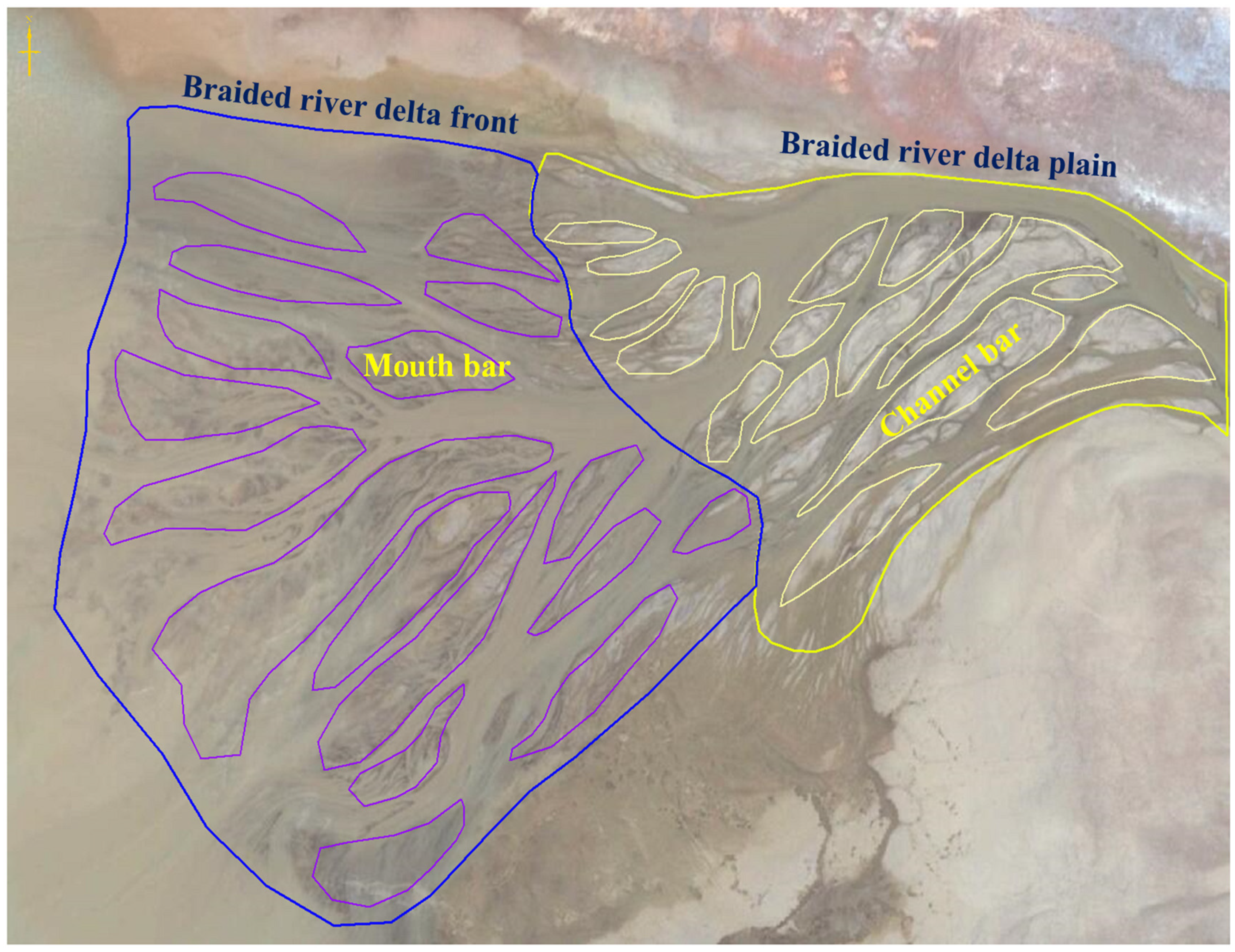
19]. In the high-resolution satellite photos in
Figure 9, the shape of the geobody represents the spatial relationships between the facies combinations. In this study, we divided the whole image into two large facies, which were the delta plain and the delta front. The delta plain consisted of channel bars and overwater distributary channels, while the delta front consisted of mouth bars and underwater distributary channels (
Figure 9).
In the delta plain training image, we first drew the channel bar geometry shapes onto the satellite photo and then digitalized the geomorphologies of specific microfacies. The same data processing was then carried out on the delta front training image, in which the mouth bar microfacies were digitalized (
Figure 10). The ratio we used was 1:1 scaling, and the channel bars had smaller scales than the mouth bars. This information was a vital reference for the scaling settings of the microfacies in the MPS geomodeling.
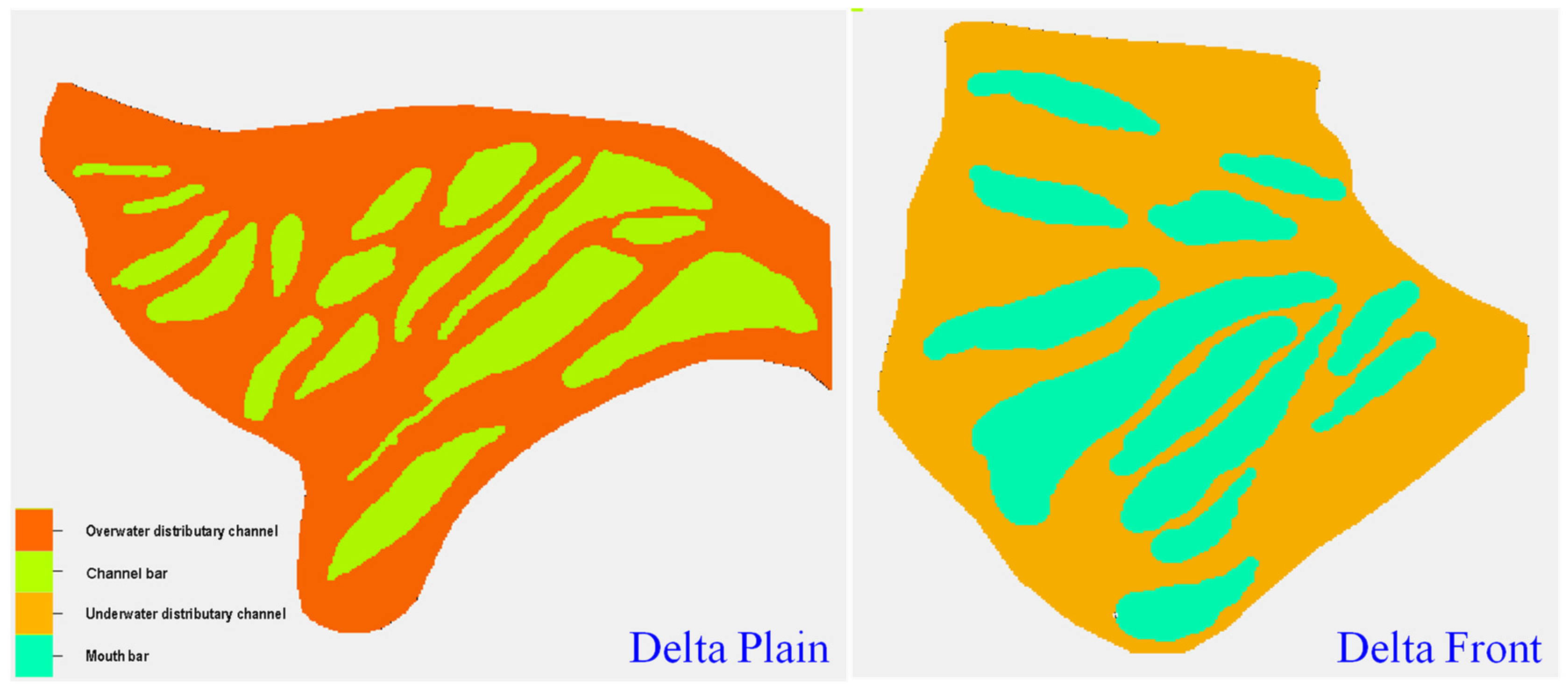
The MPS geomodeling in this study was also an iterative process. We simulated four microfacies, which were overwater distributary channels with channel bars in the delta plain and underwater distributary channels with mouth bars in the delta front.
The large facies framework constrained the areas of the microfacies within the four layers. The training image catalog initially consisted of a small set of microfacies associations [
20], and the training images were used to define the relationships between the individual facies. The MPS patterns used in this study were created using the delta plain and delta front training images. Finally, the four sedimentary microfacies were modeled, i.e., the overwater distributary channels with channel bars and the underwater distributary channels with mouth bars. The results showed that the mouth bars were larger than the channel bars overall, which was consistent with the observations from the satellite photos. The widths of the mouth bars ranged from 58 m to 733 m, while their lengths ranged from 116 m to 2566 m. The widths of the channel bars ranged from 45 m to 264 m, while their lengths ranged from 56 m to 1236 m. As the delta plain retrogradation process occurred from T
2a
1-1-4 to T
2a
1-1-1, the delta front would have taken up all of the study area, which is the root cause of why only underwater distributary channels and month bar sediments appeared during the T
2a
1-1-1 period (
Figure 11).
3.2. Three-Dimensional Interbed Geomodeling
The interbed geomodeling presented a big challenge in this study, especially because the reservoir had a strong lateral heterogeneity. Firstly, we classified the interbeds as muddy or calcareous interbeds, based on core samples. The interbed features could be identified qualitatively and quantitatively using the well logs, such as GR, SP, AC, CNL, DEN, and porosity [
21]. In this study, the muddy interbeds had relatively high GR, SP, and DEN values and low AC and CNL values, with porosity values of more than 0.15 but less than 0.185 and GR values of more than 65 API. The calcareous interbeds had relatively low GR, SP, AC, and CNL values and relatively high DEN values, with porosity values of less than 0.15 (
Figure 12).
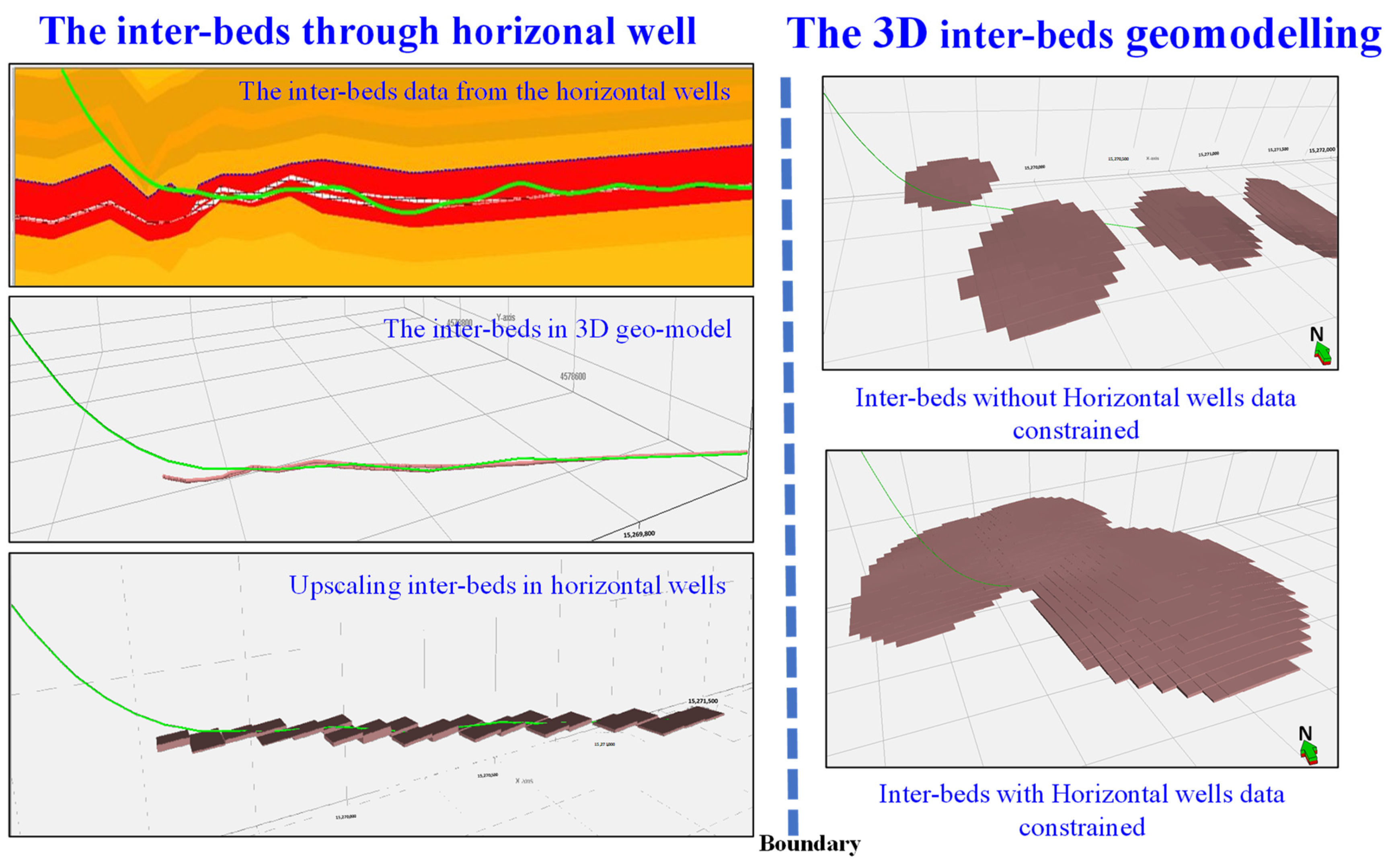
The resistivity inversion results from the 32 horizontal wells provided consolidated evidence for the determination of the interbed plane distributions [
6]. Therefore, the distribution ranges of the interbeds could be confirmed using the well log response characteristics of the vertical wells and the resistivity inversion results of the horizontal wells. We upscaled the interbeds in the 3D geomodel to create an initial model (
Figure 13).
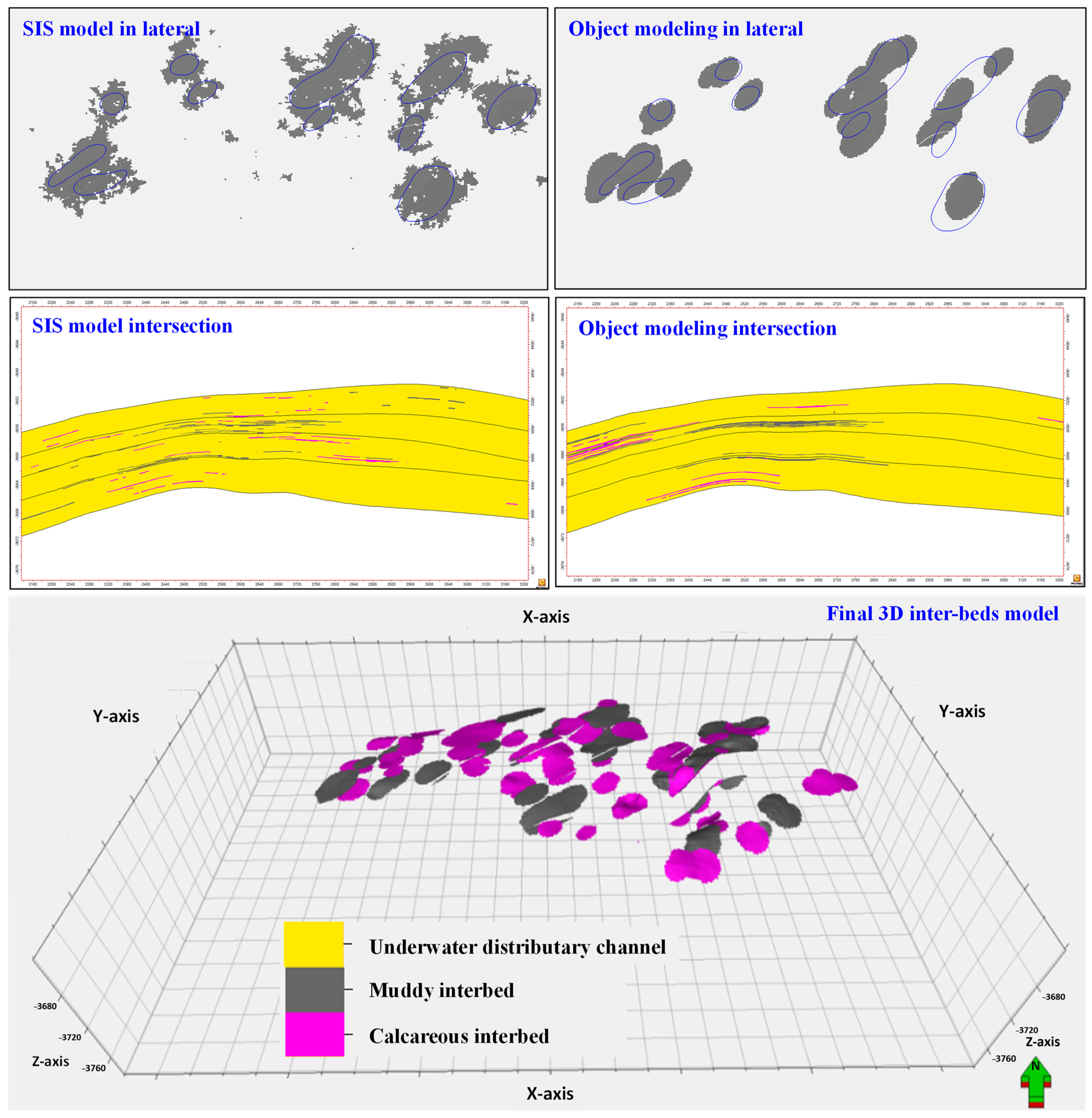
Objective modeling and sequential indicator simulation (SIS) methods have been used in interbed geomodeling as their input data are same, although object geomodeling produces more continuous and smoother results than SIS [
22]. We corrected the simulation results using the hard data from the wells. The SIS results were well dispersed and inconsistent with the observations from the horizontal wells. Therefore, the objective modeling results were selected for the interbed geomodeling in this study (
Figure 14).
3.3. The Comprehensive 3D Facies Model and Validation
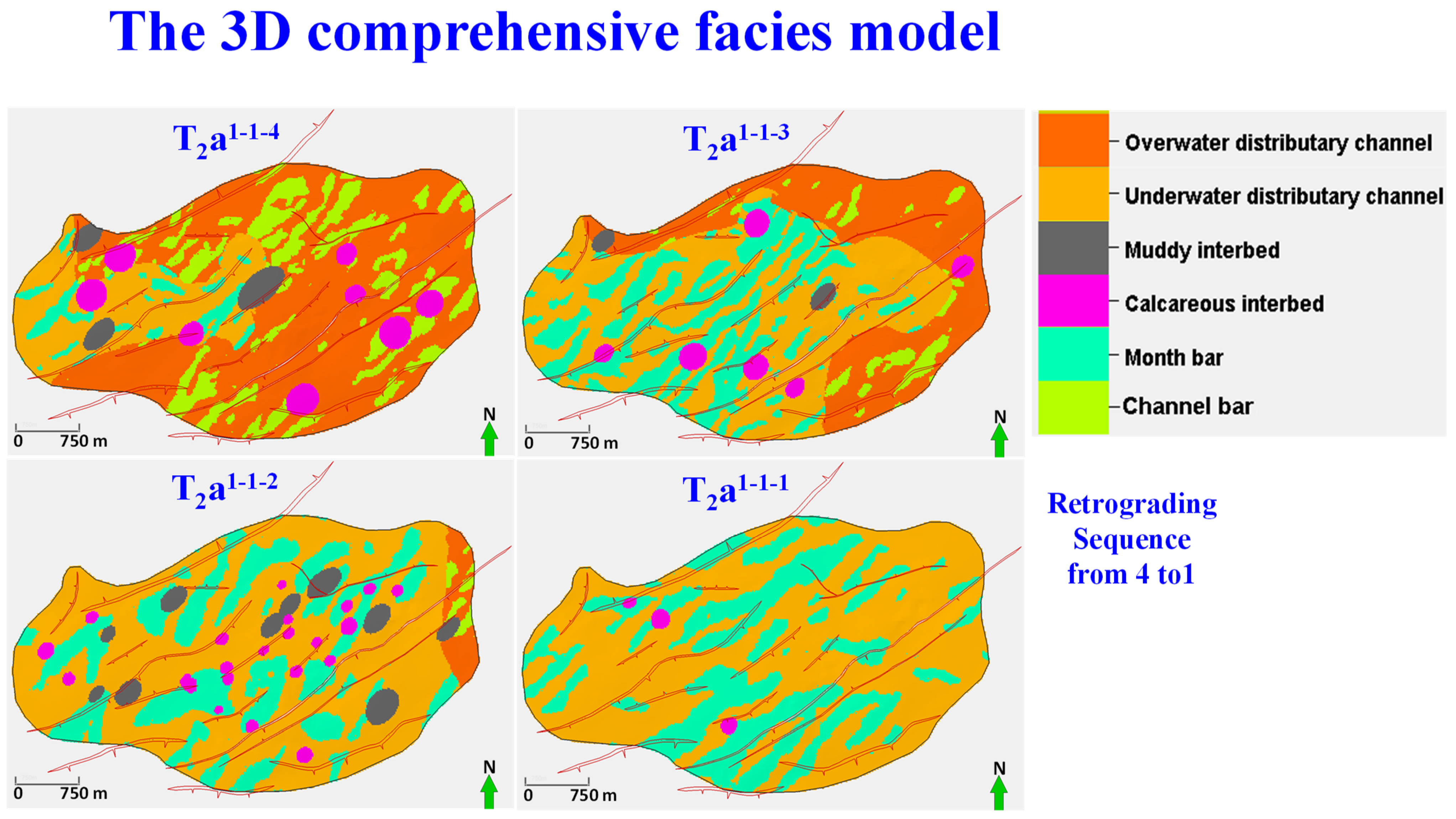
We combined the interbed model with the sedimentary facies model and called the output a comprehensive facies model. According to our geological understanding of the study area, the selected target layer was a delta front and delta plain deposition in the northeast direction. Muddy deposition could be destroyed by the power of the distributary channels, so the muddy interbeds developed in standing water environments. The same mechanism also occurred for the calcareous interbeds, which mainly developed in delta front sedimentary environments. We rarely found that interbeds developed in delta plain environments, and we could see that only a few calcareous interbeds existed in the T
2a
1-1-1 period, according to the comprehensive 3D facies model (
Figure 15).
3.4. The Facies-Controlled Property Modeling
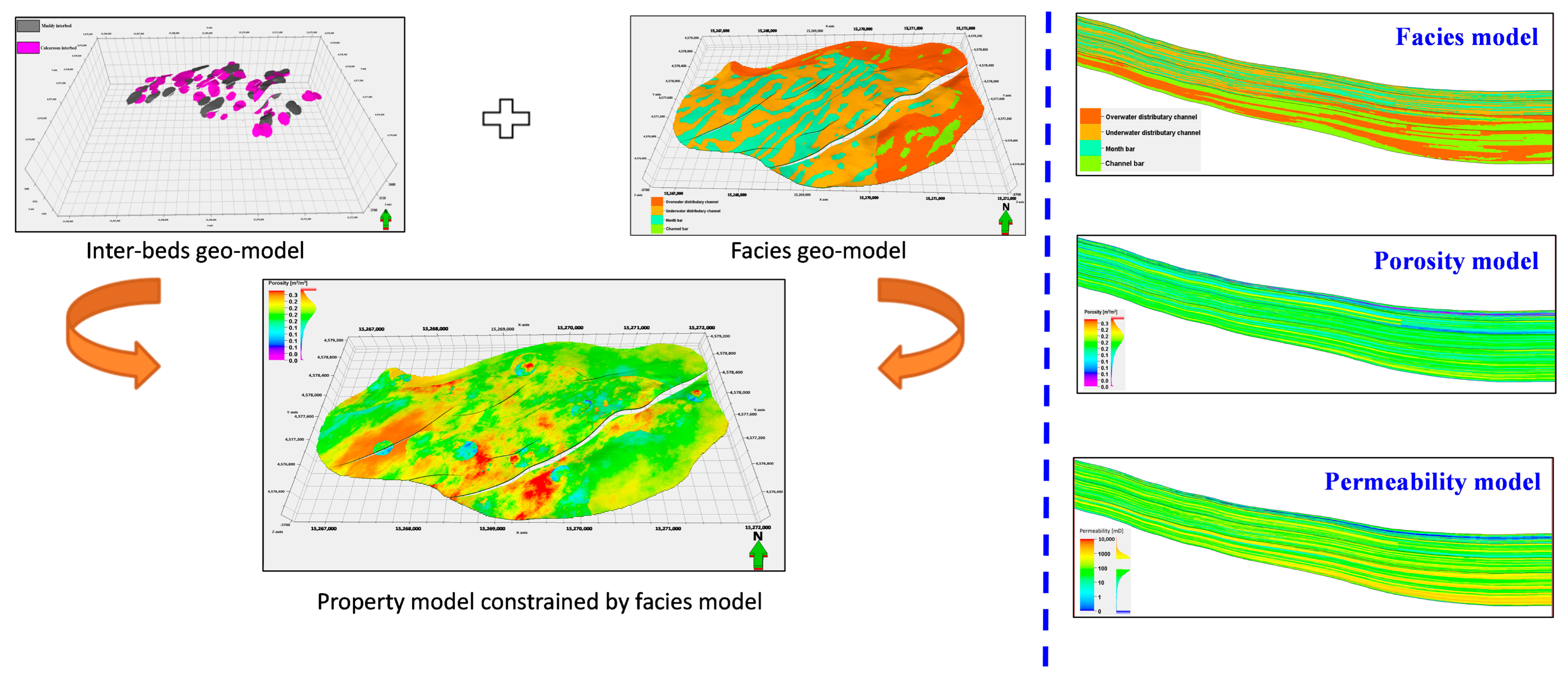
The facies-controlled property modeling had two stages (
Figure 16). The first stage was the comprehensive facies modeling, which was carried out as described previously. The reservoir rock properties were simulated by controlling the individual facies in the comprehensive facies model. We then used the hard data from the wells in the drilled area to correct the model.
In this study, we created a porosity model and a permeability model, which were directly controlled by the facies model. However, the J function was used for the water saturation modeling, which was indirectly controlled by the facies model, because the porosity and permeability models were taken as input parameters for the J function.
3.4.1. Porosity Modeling
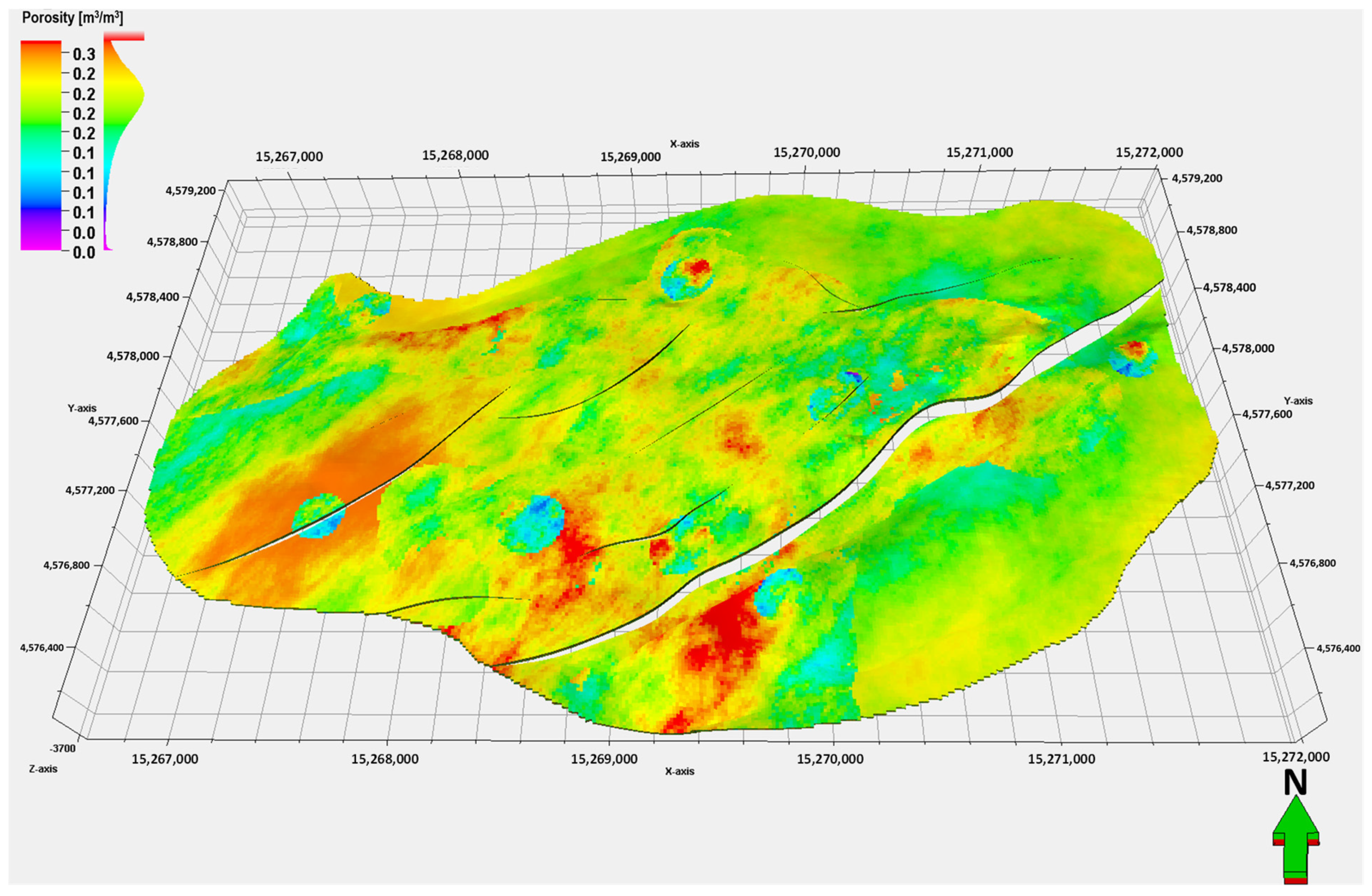
The porosity log was calculated using the Wyllie formula for wells (Equation (1)). The porosity logs were upscaled into the 3D geomodel grids as hard data, and the Gaussian random function simulation method controlled by the facies model was used for the porosity modeling. The porosity model showed a strong correlation with the facies model, and the porosity value range was 0~0.36. The interbed area had a relatively low average porosity value of about 0.06. The mouth bar and channel bar areas showed higher porosity values (
Figure 17). The results were validated using coreflooding laboratory data.
The Wyllie formula is presented below [
23]:
where
ACf is the fluid acoustic slowness (which was equal to189 μs/ft),
ACma is the sandstone skeleton slowness (which was equal to 55 μs/ft), and
ACsh is the mudstone skeleton slowness in μs/ft.
3.4.2. Permeability Modeling
In this study, the permeability well logs were calculated using the Timur formula. The rock properties of the core samples were divided into two segmentations, according to the relationships between porosity and permeability. The
SWI values of the two segmentations were different (
Figure 18 and Equation (2)). The data points used in the Timur formula fitting were taken from laboratory core data. Firstly, the permeability well logs were upscaled in the 3D geomodel grids as hard data and the Gaussian random function simulation method, which was constrained by the facies model and the trends of the porosity model, were used for the permeability modeling. In the final model, the permeability value range was 0.1~1000 mD, which was similar to the trend seen in the 3D porosity model, although there was a difference in the eastern area because the permeability did not always have a linear correlation with the porosity model. The microfacies could affect the permeability distribution, and the interbed areas had much lower permeability values compared to other areas (
Figure 19). The analytical equation for permeability showed that during the initial period, permeability increased almost nonlinearly according to exponential law and then increased almost linearly or stabilized. The results were validated using coreflooding laboratory data [
24].
The Timur formula is presented below [
25]:
where
PERM is the permeability (mD),
POR is the porosity (%), and
SWI is the irreducible water saturation (%). When
POR < 20%, then
SWI = 30%, and when
POR ≥ 20%, then
SWI = 13%.
3.4.3. Water Saturation Modeling
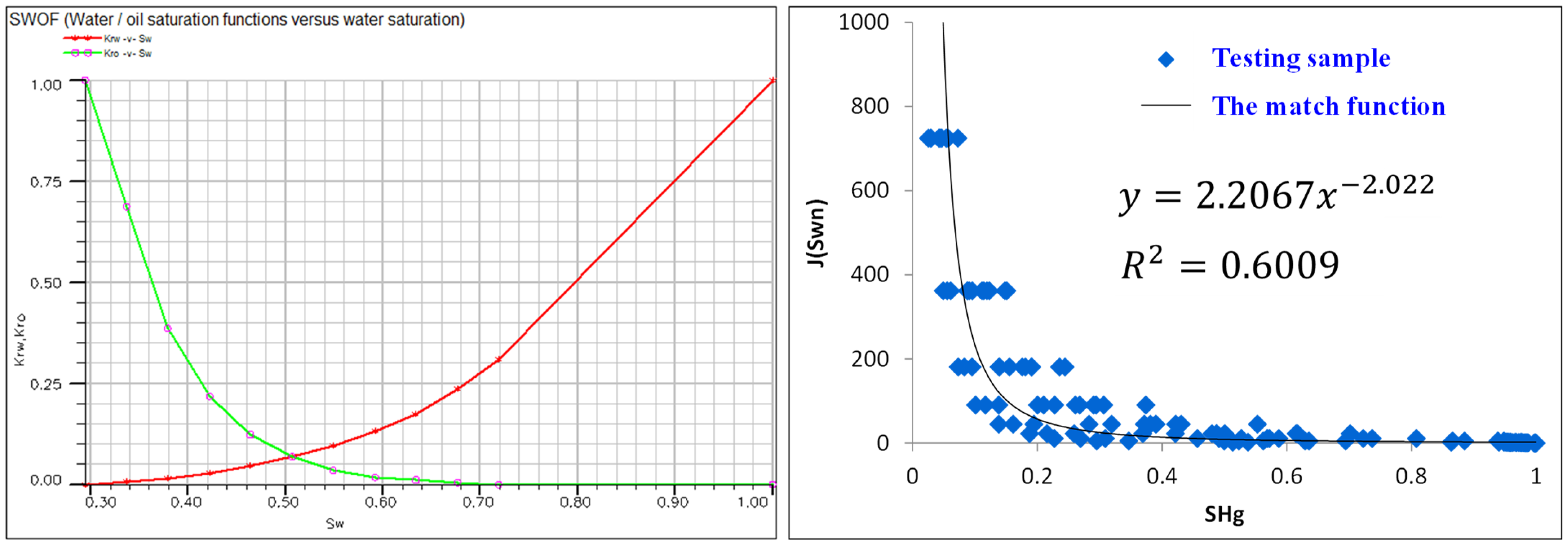
The water saturation model was calculated using the J formula. According to the statistics of the phase-to-osmosis data, the irreducible water saturation was 0.294 (
Figure 20; left map), and the average capillary pressure curve was obtained using the J function (
Figure 20; right map). The water saturation calculations were derived using Equation (3). The detailed process of deriving Equation (3) was not important to this study, although some specific cases have been presented in other public papers [
26]. The water saturation model was corrected using the water saturation data from the wells. The
Sw model produced lower water saturation values in the higher elevation parts of the reservoir, which matched the actual observations of the drilled area (
Figure 21)
.The water saturation formula is presented below [
27]:
where
SW is the water saturation (%),
H is the liquid column height (m),
K is the permeability (mD), and
is the effective porosity (%).
4. Field Development Analysis Results
Based on our research results, we proposed a novel approach for enhancing geomodeling accuracy for complex geological facies. According to the established three-dimensional geological model of the study area, the oil volume of the original oil in place (OOIP) was calculated using the volumetric method, and the geological reservoir volume was calculated using the current geomodel, which was then compared to previous publicly released reservoir volume calculation results. The relative error was only about 2.4%, which indicated that the proposed 3D geological model had high accuracy.
Based on historic math and reservoir simulation results, the reservoir volume calculation in our dynamic analysis was very close to that of the statistic geological model reservoir. The relative error was only 0.92%, which met the requirements for fitting accuracy. Based on historic matching, dynamic predictions were carried out, and various production parameters were measured, such as liquid production, oil production, water content, and reservoir pressure. In the historic matching, the dynamic parameters of the numerical simulation results were very similar to the actual measured parameters from the Tahe Oilfield B9 area, and the overall compliance rate was more than 95%, which comprehensively verified the reliability of the proposed 3D geological modeling approach (
Figure 22).
5. Discussion
In general, classical two-point statistics methods have been used for thin interbed reservoir simulations, such as the sequential indicator simulation algorithm based on logging data; however, these approaches are unable to simulate complicated reservoir properties in detail [
2]. In this study, we used the multipoint facies simulation (MPFS) algorithm as an embedded method for microfacies. The MPFS algorithm is a pixel-based algorithm that creates facies models that can replicate object models. The principal idea of the MPFS algorithm is the description of spatial correlations from one-to-many points at the same time as opposed to two-point statistics (i.e., point-to-point statistics, such as kriging or stochastic simulations). The variograms can then be replaced using 2D or 3D training images. Training images describe the spatial correlations from one-to-many points (i.e., for facies and their relative positions). The MPFS algorithm is a sequential simulation algorithm that can use more complicated statistical distributions for the simulation of facies distributions compared to two-point geostatistics methods, such as sequential indicator simulation (SIS). The main advantage of the MPFS method is that it is capable of producing models that are considerably more geologically complex than SIS. The advantage of the MPFS method compared to object modeling is that it is pixel-based; so, it is capable of conditioning data more easily than Boolean models. However, when training images cannot reveal the real correlations between the facies within a study area, the simulations could be ridiculous [
11] (Schlumberger, 2016). In this study, we created many MPFS realizations. The challenge was to find the proper I/J/K scaling and rotation degree for the simulations. We determined the parameters based on a scaling comparison between the geometric shapes shown on the satellite photos and the simulated microfacies, so it was a repeated trial-and-error process.
The residual oil distributions interacted with the microfacies, interbed distributions, and development wells. The interbeds played blocking roles in the seepage of the oil, so the upper and lower parts of the interbeds were often enriched with residual oil. Therefore, the residual oil was directly jointly controlled by the interbeds and the development wells during oilfield production. Meanwhile, the microfacies indirectly controlled the potential oil volume in the study area. The drilling and production data validated these results, which helped us to develop recommendations for geomodel quality improvements.
6. Conclusions
This study proposed an embedded workflow for an integrated geomodel accuracy enhancement solution, which was developed at the Tahe Oilfield. A comprehensive facies model was simulated using a multiscale joint controlled strategy on the wells (Point), 2D sections (Line), and horizontal wells (Surface). The horizontal well resistivity inversion results could control lateral interbed distributions. This method accurately described the 3D distribution areas of the thin interbeds in the study area. The simulated interbeds were fitted to the real geometry of the subsurface interbeds, and the relationships between the microfacies were confirmed. The oil recovery rate could be increased by at least 2.85% using our accurate geomodel. The field development results validated the geomodel accuracy, based on dynamic production data from the wells. Overall, we drew the following conclusions from this study:
An embedded MPS geomodeling process within the hierarchical mindset is necessary for more reasonable geomodels of complicated sedimentary environments, such as quick delta transition sequences;
Using horizontal well data can characterize lateral interbed distributions better than vertical well data;
Comprehensive facies models are required to control property modeling and create accurate property models (i.e., lithofacies plus sedimentary microfacies-controlled modeling).
This integrated geomodel accuracy enhancement solution could be fundamental to proposed adjustment scenarios for future oilfield development, such as drilling new wells in potential areas, artificial lift measurements for drilled wells, etc. In our next study, accurate geomodels will form machine learning training datasets for sweetness predictions, in which well pattern designs will be predicted in geological sweet spots using AI technology.
Author Contributions
Conceptualization, L.K., T.D. and F.R.; Methodology, F.R., L.K. and L.Z.; Software, L.Z. and F.R.; Validation, T.D., Z.L., X.W. and L.Z.; Formal analysis, F.R. and L.Z.; Investigation, L.K., T.D. and Z.L.; Resources, T.D., Z.L. and X.W.; Data curation, T.D. and L.Z.; Writing—original draft preparation, F.R.; Writing—review and editing, F.R. and L.Z.; Visualization, F.R.; Supervision, L.K., Z.L. and X.W.; Project administration, L.K. and T.D. All authors have read and agreed to the published version of the manuscript.
Funding
This research received no external funding.
Data Availability Statement
The data are unavailable due to privacy and ethical restrictions.
Acknowledgments
This research was supported by the SINOPEC Northwest Petroleum Bureau. We gratefully acknowledge and appreciate the productive work and cooperation from colleagues at SINOPEC Northwest as they shared a lot of practical experience and dynamic geological understanding of the oilfield with us. We would also like to thank the three anonymous reviewers for their comments and suggestions, which greatly improved the manuscript.
Conflicts of Interest
The authors declare no conflict of interest.
References
- Li, Y. Comprehensive Tapping Residual Oil Potential of Strong Water Drive Mature Oilfield in Southern American Rainfall Region. In Proceedings of the International Oil and Gas Conference and Exhibition in China, Beijing, China, 8–10 June 2010; p. SPE131883. [Google Scholar]
- Yu, P. Facies-Controlled Modeling for Permeability of Tight Gas Reservoir Based on Hydrodynamic and Geophysics Characteristics. Geofluids 2022, 2022, 5033078. [Google Scholar] [CrossRef]
- Wu, T.; Yingmin, W.; Lei, Z. Forebulge migration and evolution of the Triassic in Tarim Basin. J. Palaeogeogr. 2013, 15, 219–230. [Google Scholar] [CrossRef]
- He, T.; Duan, T.; Zhao, L.; Liu, Y. Triassic sedimentary model in Block T of Tahe oilfield, Tarim Basin. J. Oil Gas Geol. 2019, 40, 822–834. [Google Scholar] [CrossRef]
- Tingting, H.; Lei, Z.; Xin, T.; Dongxu, H. An application of sedimentation simulation in Tahe oilfield. IOP Conf. Ser. Earth Environ. Sci. 2017, 100, 012185. [Google Scholar] [CrossRef]
- Tingting, H.; Taizhong, D.; Lei, Z.; Song, H.; Yanhua, L. Interlayer identification and distribution of Triassic lower oil group in block 9 of Tahe oilfield. J. Northeast. Pet. Univ. 2017, 41, 26–35,122. [Google Scholar]
- Zheng, M.L.; Wang, Y.; Jin, Z.J.; Li, J.C.; Zhang, Z.P.; Jiang, H.S.; Xie, D.Q.; Guo, X. Superimposition, evolution and petroleum accumulation of Tarim basin. J. Oil Gas Geol. 2014, 35, 925–933. [Google Scholar] [CrossRef]
- Ying-Yue, Z.; Hanming, G.; Chengguo, C. Characteristics of seismic response to triassic sandstone reservoirs in the Tahe oilfield. Nat. Gas Ind. 2008, 28, 52–55, 146. [Google Scholar]
- Strebelle, S. Conditional simulation of complex geological structures using multiple-point statistics. Math. Geol. 2002, 34, 1–21. [Google Scholar] [CrossRef]
- Zhang, T.F.; Switzer, P.; Journel, A. Filter-based classification of training image patterns for spatial simulation. Math. Geol. 2006, 38, 63–80. [Google Scholar] [CrossRef]
- Tuanfeng, Z.; Ting, L.; Stacy, R.; Grace, Y.; Manoj, T. An Integrated Multipoint Statistics Modeling Workflow Driven by Quantification of Geological Analogue Database. In Proceedings of the 73rd EAGE Conference and Exhibition incorporating SPE EUROPEC 2011, Vienna, Austria, 23–27 May 2011. [Google Scholar]
- Kaplan, R.; Pyrcz, M.J.; Strebelle, S. Deepwater reservoir connectivity reproduction from MPS and process-mimicking geostatistical methods. In Geostatistics Valencia 2016; Springer International Publishing: Berlin/Heidelberg, Germany, 2017; Volume 19, pp. 601–611. [Google Scholar]
- Walsh, D.A.; Manzocchi, T. A method for generating geomodels conditioned to well data with high net: Gross ratios but low connectivity. Mar. Pet. Geol. 2021, 129, 105104. [Google Scholar] [CrossRef]
- Zhang, L.; Manzocchi, T.; Ponten, A. Hierarchical parameterisation and modelling of deep-water lobes. In Proceedings of the Petroleum Geostatistics, Biarritz, France, 7–11 September 2015. [Google Scholar] [CrossRef]
- Xu, W.; Fang, L.; Zhang, X.Y.; Wang, P.; Liu, J. Object-based 3D geomodel with multiple constraints for early Pliocene fan delta in the south of Lake Albert Basin, Uganda. J. Afr. Earth Sci. 2017, 125, 1–10. [Google Scholar] [CrossRef]
- Falivene, O.; Arbués, P.; Howell, J.; Muñoz, J.A.; Fernández, O.; Marzo, M. Hierarchical geocellular facies modelling of a turbidite reservoir analogue from the Eocene of the Ainsa basin, NE Spain. Mar. Pet. Geol. 2006, 23, 679–701. [Google Scholar] [CrossRef]
- Rattazzi, S.; Hansen, A. Discrete-NTG Truncated Gaussian Simulation: An Alternative Modeling Approach for Coal-Seam-Gas Unconventional Reservoirs, Bowen Basin, Eastern Australia. SPE Reserv. Eval. Eng. 2020, 23, 854–864. [Google Scholar] [CrossRef]
- Shang, W.; Xu, S.; Mao, Z.; Li, X.; Gao, G.; Li, Z.; Qin, L. High-resolution sequence stratigraphy in continental lacustrine basin: A case of Eocene Shahejie formation in the Dongying Depression, Bohai Bay Basin. Mar. Pet. Geol. 2022, 136, 105438. [Google Scholar] [CrossRef]
- Rezaee, H.; Marcotte, D.; Tahmasebi, P.; Saucier, A. Multiple-point geostatistical simulation using enriched pattern databases. Stoch. Environ. Res. Risk Assess. 2015, 29, 893–913. [Google Scholar] [CrossRef]
- Carrillat, A.; Sharma, S.K.; Grossmann, T. Geomodeling of Giant Carbonate Oilfields with a new Multipoint Statistics Workflow. In Proceedings of the Abu Dhabi International Petroleum Exhibition and Conference, Abu Dhabi, United Arab Emirates, 1–4 November 2010; p. SPE137958. [Google Scholar]
- Wu, J.; Fan, T.; Gao, Z. Identification, origin and distributions of barriers/baffles Xing-I oil layer in Block Du-84 of the western Liaohe Depression. J. Oil Gas Geol. 2017, 38, 248–258. [Google Scholar] [CrossRef]
- Zhou, F.; Shields, D.; Tyson, S.; Esterle, J. Comparison of sequential indicator simulation, object modelling and multiple-point statistics in reproducing channel geometries and continuity in 2D with two different spaced conditional datasets. J. Pet. Sci. Eng. 2018, 166, 718–730. [Google Scholar] [CrossRef]
- Yi, H.; Jitian, Z.; Yingzhao, Z.; Minggang, G.; Lijun, W. Fluid identification based on forward modeling. Oil Geophys. Prospect. 2019, 54, 726, 867–874, 881. [Google Scholar]
- Turbakov, M.S.; Kozhevnikov, E.V.; Riabokon, E.P.; Gladkikh, E.A.; Poplygin, V.V.; Guzev, M.A.; Jing, H. Permeability Evolution of Porous Sandstone in the Initial Period of Oil Production: Comparison of Well Test and Coreflooding Data. Energies 2022, 15, 6137. [Google Scholar] [CrossRef]
- Xinlei, S.; Yunjiang, C.U.I.; Wankun, X.; Zhang, J.; Yeqin, G. Formation permeability evaluation and productivity prediction based on mobility from pressure measurement while drilling. Pet. Explor. Dev. 2020, 47, 146–153. [Google Scholar]
- Zong, D.; Yidong, Z.; Wei, L.; Zilong, J. Modeling Method of Oil Saturation Based on J Function—Taking Lufeng A as an Example. Open J. Nat. Sci. 2017, 5, 437–444. [Google Scholar] [CrossRef]
- Shao, C.R.; Zhang, P.F.; Zhang, F.M. Improving well log evaluation accuracy of tight sandstone gas saturation using J function. J. China Univ. Pet. 2016, 40, 57–65. [Google Scholar]
Figure 1.
A structural map of the Tarim Basin and the B9 area of the Tahe Oilfield, located in the Shaya uplift.
Figure 1.
A structural map of the Tarim Basin and the B9 area of the Tahe Oilfield, located in the Shaya uplift.
Figure 2.
The history of sedimentary evolution in the area, from previous research (Reprinted with permission from Ref. [
6], 2017, Tingting He, Taizhong Duan et al.).
Figure 2.
The history of sedimentary evolution in the area, from previous research (Reprinted with permission from Ref. [
6], 2017, Tingting He, Taizhong Duan et al.).
Figure 3.
A structural map of the Tahe Oilfield B9 area (the purple block is the Tahe Oilfield B9 area, which is intersected by several normal faults).
Figure 3.
A structural map of the Tahe Oilfield B9 area (the purple block is the Tahe Oilfield B9 area, which is intersected by several normal faults).
Figure 4.
A well section profile from the Tahe Oilfield B9 area.
Figure 4.
A well section profile from the Tahe Oilfield B9 area.
Figure 5.
The integrated workflow presented in this study (in this flowchart, the key steps or outputs are presented, and the highlighted object modeling was the final method used for the interbed geomodeling).
Figure 5.
The integrated workflow presented in this study (in this flowchart, the key steps or outputs are presented, and the highlighted object modeling was the final method used for the interbed geomodeling).
Figure 6.
The sequence stratigraphy division of the wells (well correlation was the basis for the rhythm section identification of T2a1-1-1, T2a1-1-2, T2a1-1-3, and T2a1-1-4 in the B9 area).
Figure 6.
The sequence stratigraphy division of the wells (well correlation was the basis for the rhythm section identification of T2a1-1-1, T2a1-1-2, T2a1-1-3, and T2a1-1-4 in the B9 area).
Figure 7.
The geometry settings in the TGS with trends simulation method (in the 2D maps, the black boundaries show the Tahe Oilfield B9 area).
Figure 7.
The geometry settings in the TGS with trends simulation method (in the 2D maps, the black boundaries show the Tahe Oilfield B9 area).
Figure 8.
The level 1 sedimentary facies framework of the study area.
Figure 8.
The level 1 sedimentary facies framework of the study area.
Figure 9.
High-resolution satellite photos of the Tahe Oilfield, taken from Google Earth.
Figure 9.
High-resolution satellite photos of the Tahe Oilfield, taken from Google Earth.
Figure 10.
The training image (TI) used in the MPS simulation (the left TI pattern represents the delta plain, while the right TI pattern represents the delta front, and the four microfacies are shown by the different colors and geometries).
Figure 10.
The training image (TI) used in the MPS simulation (the left TI pattern represents the delta plain, while the right TI pattern represents the delta front, and the four microfacies are shown by the different colors and geometries).
Figure 11.
The results of the four layers of the MPS microfacies modeling.
Figure 11.
The results of the four layers of the MPS microfacies modeling.
Figure 12.
The interbed features identified from the well data.
Figure 12.
The interbed features identified from the well data.
Figure 13.
The interbed distributions, confirmed by the horizonal well data.
Figure 13.
The interbed distributions, confirmed by the horizonal well data.
Figure 14.
The interbed geomodels built using the two methods (the gray color represents the muddy interbeds, and the purple color represents the calcareous interbeds in the 3D interbed models).
Figure 14.
The interbed geomodels built using the two methods (the gray color represents the muddy interbeds, and the purple color represents the calcareous interbeds in the 3D interbed models).
Figure 15.
The comprehensive 3D facies model of the rhythm layers (showing two lithofacies and four microfacies).
Figure 15.
The comprehensive 3D facies model of the rhythm layers (showing two lithofacies and four microfacies).
Figure 16.
The property modeling, which was constrained by the facies model.
Figure 16.
The property modeling, which was constrained by the facies model.
Figure 17.
The 3D porosity model.
Figure 17.
The 3D porosity model.
Figure 18.
The porosity vs. permeability cross-plot analysis for the core well data.
Figure 18.
The porosity vs. permeability cross-plot analysis for the core well data.
Figure 19.
The 3D permeability model.
Figure 19.
The 3D permeability model.
Figure 20.
The statistics of the phase-to-osmosis data.
Figure 20.
The statistics of the phase-to-osmosis data.
Figure 21.
The 3D water saturation model (the higher water saturation values are represented by the blue color.).
Figure 21.
The 3D water saturation model (the higher water saturation values are represented by the blue color.).
Figure 22.
The reservoir simulation results using the proposed 3D geomodel (the dashed lines marked with H are from history-matched data, and the solid lines are from the actual production data).
Figure 22.
The reservoir simulation results using the proposed 3D geomodel (the dashed lines marked with H are from history-matched data, and the solid lines are from the actual production data).
Table 1.
A brief geological stratigraphy of the study area.
Table 1.
A brief geological stratigraphy of the study area.
| System | Group | Long-Term Cycle | Medium-Term Cycle | Short-Term Cycle |
|---|
| Section | Sandy Layer | Rhythm Section |
|---|
| Triassic | Upper | Halahatang | T3h2 | | |
| T3h1 | | |
| Middle | Akkol | T2a4 | | |
| T2a3 | | |
| T2a2 | | |
| T2a1 | T2a1-1-1 | T2a1-1-1 |
| T2a1-1-2 |
| T2a1-1-3 |
| T2a1-1-4 |
| T2a1-2 | … |
| … |
| Lower | Ketur | T1k | | |
| Disclaimer/Publisher’s Note: The statements, opinions and data contained in all publications are solely those of the individual author(s) and contributor(s) and not of MDPI and/or the editor(s). MDPI and/or the editor(s) disclaim responsibility for any injury to people or property resulting from any ideas, methods, instructions or products referred to in the content. |
© 2023 by the authors. Licensee MDPI, Basel, Switzerland. This article is an open access article distributed under the terms and conditions of the Creative Commons Attribution (CC BY) license (https://creativecommons.org/licenses/by/4.0/).


