Simple and Accurate Model of Thermal Storage with Phase Change Material Tailored for Model Predictive Control

Abstract

Thermal heat storage is becoming important in systems with renewable energy sources. Their largest benefit is smoothing the intermittent production and reduction in the site peak demand. The advantages of thermal energy storage with phase-change material are storing energy at a lower temperature for reduction in thermal losses, and enabling energy transfer at a constant temperature, which reduces the risk of equipment damage. In this paper, a low-order model of latent thermal energy storage, derived in a state-space form by using the mixed logical dynamical approach, is proposed. The model is compared to a stratified model and shows significant improvements of physical accuracy and execution time. Finally, a model predictive control algorithm suited for the real case study is designed, implemented and compared to classical rule-based control. The obtained results show significant energy savings of 8.43%, and improvements in user comfort and equipment duration.

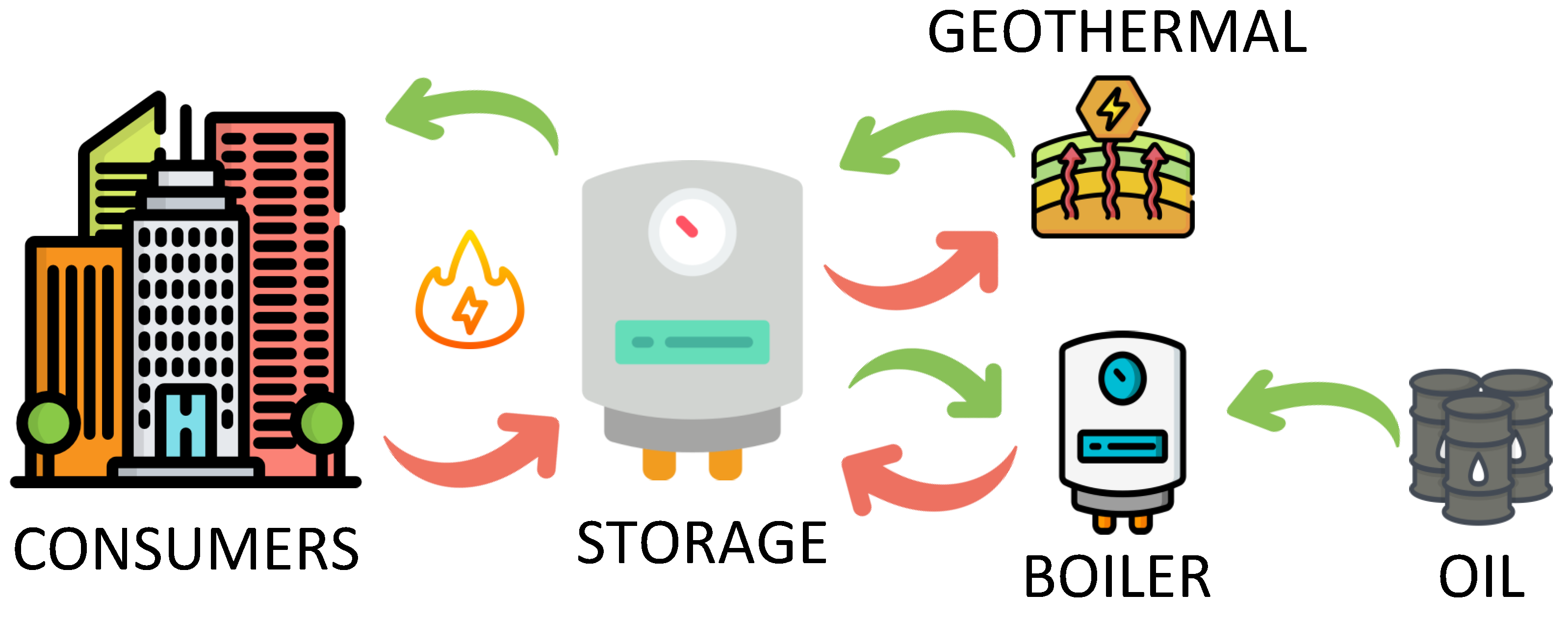
1. Introduction

The last eight years have been the warmest recorded in history, while the annual average temperature has become 1.2 ${}^{\circ }\mathrm{C}$ higher in comparison to the 1850–1900 period [1]. In 2022, atmospheric carbon dioxide concentrations increased by approximately 2.1 ppm, similar to the rates of recent years. Moreover, greenhouse gases increased by 3% in the second quarter of 2022, compared with the same quarter of 2021 [2]. The building sector is a key contributor to greenhouse gases emission, representing around one third of energy-related EU emissions [3]. Numerous policies and initiatives directed towards their energy efficiency increase have emerged. The EU 2030 Energy Strategy, which is based on the encouraging achievements and well-accepted research and implementation trends of the preceding 20-20-20 strategy (${\mathrm{CO}}_2$ emissions reduction—renewables share—energy savings), aims for 55% emissions reduction by 2030 [4]. This strategy mostly depends on reducing energy waste, which can be accomplished by employing thermal energy storage (TES) to bridge the gap between energy production and consumption. TES enables energy delivery to the system when energy production becomes expensive or inefficient, which leads to better energy efficiency and economic savings. On the other hand, TESs store energy in favorable energy generation conditions when there is no demand. Additionally, TES is crucial to the utilization of renewable energy sources (RESs) since it can effectively smoothen their intermittent energy production. The reduction in site peak demand is possible if TES is connected to a renewable source and utilized in conjunction with another conventional energy source as it is shown in [5].

Recently, there has been notable focus placed on latent TES, which use phase-change material (PCM) to store energy. According to the research from K. Pielichowska et al. [6], their key benefit is the ability to supply energy that is highly concentrated while maintaining the TES at lower temperatures. Achieving high energy efficiency in this type of storage is greatly influenced by the material selection. According to [7,8,9], some of the required material properties are good heat transfer, small volume change, high density, long-term chemical stability, no toxicity, and no fire hazard. The benefits of including PCM in TES operating with solar heat are explained in [10,11,12]. The techno-economic feasibility of implementing PCMs in TESs was given in the study from S. Mazzoni et al. [13]. Building operations and associated expenses are substantially less affected by large fluctuations in land rental price when phase change materials are used. Moreover, S. Baek et al. [14] show that PCM can be utilized to save energy in radiant floor heating systems. For instance, applying 20–50 mm of PCM leads to 7.3–15.3% of energy savings. Furthermore, it is possible to combine latent TES with other storage types, such as Ruth steam storage, as it is presented in the work from R. Hofmann et al. [15], where the combination compensates for the disadvantages of individual storage types.

However, the method for obtaining a simple but precise model of latent storage suitable for advanced control algorithms has still not been established. C. R. Touretzky et al. [16] base their model on temperature-enthalpy correlation. Because it is continuous throughout the phase transition process, they use enthalpy as a time-dependent function. Their model is suitable for advanced control strategies, such as model predictive control (MPC). However, it limits the possibility of achieving a solution in real time because it adds additional binary variables, which increases the computational complexity. In [17,18], a geometry model of latent storage is created by using the meshing methods. These models are physically very precise but they are not suitable for control purposes because their complexity significantly extends the control algorithm computation time. The latent TES model presented by M. Shanks et al. [19] is usable for the recharging and discharging strategy. However, calculations take only temporary values into account, and they do not use thermal load predictions. In the study from Yang et al. [20], the thermal model of latent TES is transformed into an analogous resistive–capacitive model as a high-order model. A. Chuttar et al. [21] implement a model employing techniques based on artificial intelligence (AI). They achieve high accuracy, but because the model is not mathematically exact, it is not applicable to MPC. The non-linear model proposed by V. Dermardiros et al. [22] is non-linear, and thus it is too complex for the practical implementation of advanced control algorithms. A stratified model that we propose in [23] is physically accurate but contains a significant number of continuous and integer variables, which deteriorates the calculation speed. Moreover, it allows the PCM energy to exceed the predefined limits.

Due to the complexity of the latent TES models, the implementation of a control algorithm is very challenging. The control algorithm in the study from G. Gholamibozanjani et al. [24] is based on IF-THEN-ELSE conditional logic. This algorithm is fast, but it does not take predictions into account, which leads to sub-optimal solutions. The hierarchical control algorithm is implemented in [25] by H. C. Pangborn et al. The upper level in it switches linear models to approximate non-linear dynamics, while the lower level leverages a fast update rate to compensate for the high-frequency disturbances and model error. However, this control algorithm regards only a process of phase change, and it cannot be used in a situation where PCM is completely melted or solidified. By applying mixed logical dynamical formulation, it is possible to implement accurate models of non-linear systems in a state-space form. A control algorithm for these models is often based on a mixed-integer problem (MIP). The MIP solution can be efficiently used for creating an optimal control schedule. In the work of A. Bürger et al. [26], MIP is used in a case of a complex thermal system that contains a heat pump and numerous energy storage types. The obtained control schedule successfully operates the system and achieves a reduction in the yearly electrical energy consumption by more than 18%. The system in the study from S. Rafii-Tabrizi et al. [27] is composed of a two-layer TES and a dual-source heat pump. It is shown that most suitable heat sources can be determined at every operating point and that the model provided in the paper is capable of reacting to variable electricity prices. In the work of F. Verrilli et al. [28], the results obtained by MIP for a district heating system with TES are compared to the results obtained by rule-based control. The MIP achieves 7% better economical cost over a 15-day horizon for the case study. J. Dorfner et al. [29] show how MIP can be implemented in the case of a whole district heating network and solutions can be still successfully found, even if the system dimensions are high. The MIP is implemented for building heating/cooling in the study of M. J. Risbeck et al. [30] and it shows lower cost and less erratic equipment usage than a similar scheme that does not employ discrete variables. F. Rukavina et al. [31] use MIP for optimal scheduling of the heat source connected to TES. They take different relations between maximal power and maximal efficiency into consideration. For every scenario, the optimal control based on MIP shows advantages in energy savings compared to the PI control (from 0.03% to 7%). In the study from K. Deng et al. [32], MIP is used for the control algorithm of a central chiller plant with thermal energy storage, and for a paper case study, daily savings of 14,130 $\mathrm{kWh}$ are achieved. The authors in [33,34] claim that by using integer control in a cooling system with ice storage device, the energy efficiency can be improved by 5–30%, depending on the case considered. D. Zhang et al. [35] show that by implementing MIP into a microgrid control, energy savings of 13% and peak power reduction of 18% are achievable. Y. Lu et al. [36] claim that the control algorithm based on MIP reduces the energy operation cost up to 47% compared with a rule-based strategy for a system with a thermal energy storage. Moreover, the on/off frequency of chillers is significantly decreased.

Considering that MIP improves energy efficiency for various cases in the field of heating and cooling, there is a motivation to apply it for the case of latent TES with a PCM material. Therefore, our motivation is to create a method for modeling energy storage with PCM in a state-space form, and also to implement the corresponding control algorithm with a high execution speed, while keeping the PCM dynamics physically accurate.

The following contributions are highlighted: $\left(i\right)$ a novel mathematical model of thermal storage with PCM based on mixed logical dynamics; $\left(ii\right)$ MPC of PCM storage energy exchange in the context of a thermal microgrid, including an oil boiler and geothermal source as energy production units, and consumers as the thermal load; and $\left(iii\right)$ detailed realistic simulations performed on the chosen test site of the public library in the city of Lendava, Slovenia. With step-by-step derivation of the thermal storage model and corresponding optimal control, the realistic results show significant impact with energy savings of 8.43%, improvement in user comfort, and extension of the equipment life span. The presented work is novel and has practical implications for developing more efficient energy systems.

This paper is organized as follows. In Section 2, modeling methods for stratified latent TES and mixed logical dynamical TES are given and compared, where the PCM dynamics logic is explained. Moreover, model parameters identification by using real data is described. The MPC control algorithm is delineated in Section 3. The simulations results are shown in Section 4, in which MPC control is compared to classical rule-based control. Section 5 concludes the paper.

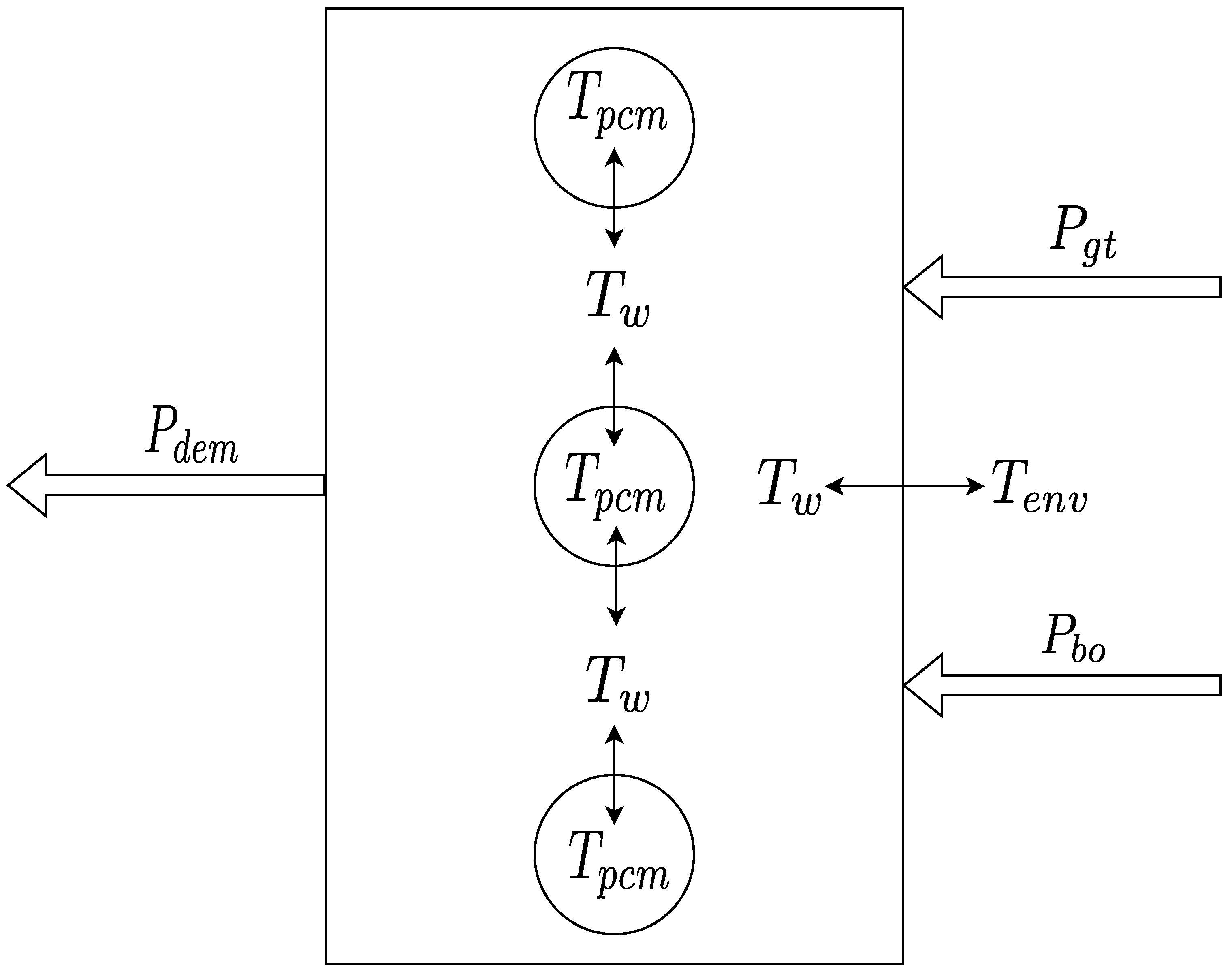
2. Thermal Storage Mathematical Model

Thermal energy storage is usually a cylindrically shaped tank filled with water. However, besides this conventional storage, energy storage can also contain thermochemical material that utilizes reversible chemical processes. On the other hand, latent storage contains PCM. It fosters huge benefits to a thermal energy system because it enables energy transfer at a constant temperature, which leads to the extension of the system’s life cycle by reducing thermal stress in the storage materials. Moreover, it can store a large amount of energy at a lower temperature. This way, geothermal sources with lower water temperatures or geothermal sources that are very distant from the storage become more efficient. Figure 1 delineates a case study of the thermal system of a public library in Lendava, Slovenia. The thermal system contains two energy sources: the first one is conventional (oil boiler), and the other one is renewable (geothermal source). The heating system of the building is connected to the geothermal source through a latent TES, which includes ATS 50 PCM material that has the phase change point at 50 ${}^{\circ }\mathrm{C}$. The emphasis is on using geothermal energy as frequently as feasible because it is free of ${\mathrm{CO}}_2$ and more economical than the oil boiler energy. However, the geothermal source cannot be used directly since the temperature of the geothermal side relies on numerous natural conditions and can occasionally be too low. Because of this, MPC is used to better utilize the geothermal source, which requires a suitable model, such as the one presented in this study.

2.1. Stratified Model

In [23], we proposed an approach for the mathematical modeling of latent heat storage based on tank stratification with several horizontal layers to obtain satisfactory model accuracy. Some of the layers contain PCM elements, and those are described by three differential equations, while layers without PCM are modeled with a single equation. These equations include energy delivery from an outside power source and energy transmittance to the thermal load. Additionally, this model physically delineates energy transfers very precisely by dividing them into thermal conduction and thermal convection. Inner flows between storage layers are modeled via mixed-integer rules given in the work of A. Bemporad et al. [37]. Moreover, PCM distinguishes two states: one regarding to the changeable energy and constant temperature, and the other for the opposite situation. The decision of which states are active is made based on the current values of the PCM temperature and energy. A significant advantage of this model is the state-space form, which makes it suitable for advanced control approaches, such as model predictive control. However, the high physical accuracy due to storage stratification leads to a significant increase in the number of continuous and integer variables in the model, which deteriorates the calculation speed. Even if the number of layers is set to only two, for some case studies, the latter model can be computationally too slow to be practically used in on-line implementation. Despite the slow computation, this model is useful for accurate simulations purposes. Another issue of the noted model is that it takes into account only temporary states of variables, which allows the latent energy of the PCM to exceed the predefined physical limits. This deviation from real behavior is shown in Figure 2, noticeable in the temperature and latent energy responses. Red dashed lines stand for the temperature of the phase change in the upper graph and for energy limits in the lower graph. In the area higher than the upper boundary, the PCM is in a liquid state. Similarly, when the energy is lower than the bottom boundary, the PCM is in a solid state. In the first period from 00:00 to 04:00, the heat storage accepts heat from an outside thermal source. When the value of 50 ${}^{\circ }\mathrm{C}$ is triggered, latent energy becomes changeable, and the temperature remains constant, which captures the slow transition from the solid to liquid phase change of the material. This happened in 00:30, but the temperature is not fixed at 50 ${}^{\circ }\mathrm{C}$ and instead it reaches about 53 ${}^{\circ }\mathrm{C}$. The obvious reason for this is the discrete time step of 15 min, and it is possible to change the submodel only in the discrete time instants. Analogously, in the period of cooling from 04:00 to 08:00, the PCM crossed temperature changes and stays at 49 ${}^{\circ }\mathrm{C}$. Also, the latent energy deviates from the predefined bounds by about 10 $\mathrm{MJ}$. During the liquid phase, the real physical value of the latent energy is 100 $\mathrm{MJ}$, while the model shows energy at 112 $\mathrm{MJ}$. Likewise, when the material becomes solid again, the latent energy reaches −9 $\mathrm{MJ}$, while it should be at 0 $\mathrm{MJ}$. As it can be seen, the system works properly from the energy perspective level, which means that system cannot create energy itself but only energy from the outside source can be gained.

2.2. Mixed Logical Dynamical Model

Drawbacks of the stratified model provide focus for further improvements of the mathematical model. The lower complexity and higher model accuracy prove to be achievable by the mixed logical dynamical approach. The main contribution of this model is that it is physically more accurate because enhancement of the PCM dynamics is achieved, so the temperature and energy limits are strictly respected. Moreover, model dimension is lower due to the simplification of the system energy flows and thermal exchange processes. This leads to faster execution, which makes the model more suitable for advanced, model-based control approaches. Model energy relations are shown in Figure 3.

Two energy sources are opted regarding the case study in Lendava: geothermal power denoted with $P_{gt}$ [$\mathrm{W}$] and oil boiler power denoted with $P_{bo}$ [$\mathrm{W}$]. The availability of $P_{gt}$ depends mostly on the geothermal source temperature denoted with $T_{gt}$ [${}^{\circ }\mathrm{C}$] and water flow denoted with $q_{gt}$ [$\mathrm{kg}$/$\mathrm{s}$]. Also, the power demand is denoted with $P_{dem}$ [$\mathrm{W}$]. For our model, regarding the case study, the number of energy inputs and outputs can be easily adjusted. The dynamics of the storage water temperature is provided with the following equation:

$$\begin{array}{ccc}\hfill m_w{c}_w\frac{d{T}_w}{dt}=P_{gt}+P_{bo}-P_{dem}-& h_{wa}{A}_{wa}(T_w-T_{env})\hfill & \\ \hfill -h_{wp}{A}_{wp}(T_w-T_{pcm}),\end{array}$$

(1)

where $T_w$ [${}^{\circ }\mathrm{C}$] is the water temperature, $T_{pcm}$ [${}^{\circ }\mathrm{C}$] is the PCM temperature, $h_{wp}$ [$\mathrm{W}$/(${\mathrm{m}}^2$$\mathrm{K}$)] is the convective heat transfer coefficient between the water and PCM, $h_{wa}$ [$\mathrm{W}$/(${\mathrm{m}}^2$$\mathrm{K}$)] is the convective heat transfer coefficient between the water and air, $A_{wp}$ [${\mathrm{m}}^2$] is the contact surface between the water and PCM, $A_{wa}$ [${\mathrm{m}}^2$] is the contact surface between the water and air, and $m_w$ [$\mathrm{kg}$] and $c_w$ [$\mathrm{J}$/($\mathrm{kg}$$\mathrm{K}$)] are the mass and specific heat of the water, respectively.

2.3. PCM Dynamics

The dynamics of the PCM temperature and energy is delineated via six independent linear submodels. At each discrete step, only one submodel is active. The activation of the submodels is decided by the combination of binary variables ${\delta }_1$, ${\delta }_2$, ${\delta }_3$ and ${\delta }_4$. They are utilized to identify different thresholds of the PCM thermal and latent energy, temperature, and their relations as explained in the sequel.

The thermal energy that can be exchanged between the PCM and water in one time step is calculated by

$$\begin{array}{c}\hfill \Delta E_{pcm}=h_{wp}{A}_{wp}(T_w-T_{pcm})T_s,\end{array}$$

(2)

where $T_s$ [$\mathrm{s}$] is the sampling time. Here, we make a small systematic error in the model because we ignore the variability of the temperature of the PCM and the water during one sampling interval, but we adhere to the law of conservation of energy—the energy that is taken to the PCM is given to the water, and vice versa. Moreover, energy is always between predefined limits, and phase change occurs precisely at a certain temperature. The variable ${\delta }_1$ describes the direction of energy by

$$\begin{array}{c}\hfill \Delta E_{pcm}\le 0\Rightarrow {\delta }_1=1,\end{array}$$

(3)

$$\begin{array}{c}\hfill \Delta E_{pcm}>0\Rightarrow {\delta }_1=0,\end{array}$$

(4)

The $T_{pcm}^{\ast }$ [${}^{\circ }\mathrm{C}$] describes the PCM temperature in the next time step in the case of changeable temperature, and not a single part of the energy is spent on increasing the latent energy. It is calculated by

$$\begin{array}{c}\hfill T_{pcm}^{\ast }=T_{pcm}+{\displaystyle \frac{h_{wp}{A}_{wp}{T}_s}{m_{pcm}{c}_{pcm}}}{T}_w-{\displaystyle \frac{h_{wp}{A}_{wp}{T}_s}{m_{pcm}{c}_{pcm}}}{T}_{pcm},\end{array}$$

(5)

where $m_{pcm}$ [$\mathrm{kg}$] and $c_{pcm}$ [$\mathrm{J}$/($\mathrm{kg}$$\mathrm{K}$)] the are mass and specific heat of the PCM, respectively.

On the other hand, $E_{pcm}^{\ast }$ [$\mathrm{J}$] denotes the PCM latent energy in the next step in the case in which energy is changeable and not a single part of the energy is spent on increasing the temperature. It is given with

$$\begin{array}{c}\hfill E_{pcm}^{\ast }=E_{pcm}+h_{wp}{A}_{wp}(T_w-T_{pcm})T_s.\end{array}$$

(6)

Variable ${\delta }_2$ represents the relation between $T_{pcm}^{\ast }$ and the temperature of change $T_{chg}$ [${}^{\circ }\mathrm{C}$] by

$$\begin{array}{c}\hfill T_{pcm}^{\ast }\le T_{chg}\Rightarrow {\delta }_2=1,\end{array}$$

(7)

$$\begin{array}{c}\hfill T_{pcm}^{\ast }>T_{chg}\Rightarrow {\delta }_2=0.\end{array}$$

(8)

Variables ${\delta }_3$ and ${\delta }_4$ show whether the latent energy in the next time step will exceed the lower limit 0 or upper limit $E_{max}$ [$\mathrm{J}$]. The following inequalities are given:

$$\begin{array}{c}\hfill E_{pcm}^{\ast }+(T_{pcm}-T_{chg})m_{pcm}{c}_{pcm}\le E_{max}\Rightarrow {\delta }_3=1,\end{array}$$

(9)

$$\begin{array}{c}\hfill E_{pcm}^{\ast }+(T_{pcm}-T_{chg})m_{pcm}{c}_{pcm}>E_{max}\Rightarrow {\delta }_3=0,\end{array}$$

(10)

$$\begin{array}{c}\hfill E_{pcm}^{\ast }+(T_{pcm}-T_{chg})m_{pcm}{c}_{pcm}\le 0\Rightarrow {\delta }_4=1,\end{array}$$

(11)

$$\begin{array}{c}\hfill E_{pcm}^{\ast }+(T_{pcm}-T_{chg})m_{pcm}{c}_{pcm}>0\Rightarrow {\delta }_4=0.\end{array}$$

(12)

Variables $z_{Ti}$ [${}^{\circ }\mathrm{C}$] and $z_{Ei}$ [$\mathrm{J}$] are the temperature outputs and the outputs of the energy submodels, ($i=1,2\dots 6$). These contionus auxiliary variables are used in MLD to represent PCM dynamics.

2.3.1. Submodel 1

The first submodel defines the situation in which PCM heats up and retains a solid state. It is activated by the following:

$$\begin{array}{c}\hfill \mathrm{IF}{\delta }_1=0\mathrm{AND}{\delta }_2=1\end{array}$$

$$\begin{array}{cc}\hfill \mathrm{THEN}& z_{T1}=T_{pcm}^{\ast }\hfill \\ & z_{E1}=0\hfill \end{array}$$

$$\begin{array}{cc}\hfill \mathrm{ELSE}& z_{T1}=0\hfill \\ & z_{E1}=0\hfill \end{array}$$

(13)

The temperature of PCM is equal to (5) and the latent energy is zero. These conditions are written in mixed logical dynamics (MLD) form by using the rules proposed in [37]. The following inequalities are given:

$$\begin{array}{cc}\hfill z_{T1}+M_T{\delta }_1& \le M_T,\hfill \end{array}$$

(14)

$$\begin{array}{cc}\hfill -z_{T1}-m_T{\delta }_1& \le -m_T,\hfill \end{array}$$

(15)

$$\begin{array}{cc}\hfill z_{T1}-M_T{\delta }_2& \le 0,\hfill \end{array}$$

(16)

$$\begin{array}{cc}\hfill -z_{T1}+m_T{\delta }_2& \le 0,\hfill \end{array}$$

(17)

$$\begin{array}{cc}\hfill z_{T1}-k{T}_w+(-1+k)T_{pcm}& \le -m_T-m_T{\delta }_1+m_T{\delta }_2,\hfill \end{array}$$

(18)

$$\begin{array}{cc}\hfill -z_{T1}+k{T}_w+(1-k)T_{pcm}& \le M_T+M_T{\delta }_1-M_T{\delta }_2,\hfill \end{array}$$

(19)

$$\begin{array}{cc}\hfill z_{E1}+M_E{\delta }_1& \le M_E,\hfill \end{array}$$

(20)

$$\begin{array}{cc}\hfill -z_{E1}-m_E{\delta }_1& \le -m_E,\hfill \end{array}$$

(21)

$$\begin{array}{cc}\hfill z_{E1}-M_E{\delta }_2& \le 0,\hfill \end{array}$$

(22)

$$\begin{array}{cc}\hfill -z_{E1}+m_E{\delta }_2& \le 0,\hfill \end{array}$$

(23)

$$\begin{array}{cc}\hfill z_{E1}+m_E{\delta }_1-m_E{\delta }_2& \le -m_E,\hfill \end{array}$$

(24)

$$\begin{array}{cc}\hfill -z_{E1}-M_E{\delta }_1+M_E{\delta }_2& \le M_E.\hfill \end{array}$$

(25)

with $k={\displaystyle \frac{h_{wp}{A}_{wp}{T}_s}{m_{pcm}{c}_{pcm}}}$. The maximum PCM latent energy and temperature are denoted by $M_E$ [$\mathrm{J}$] and $M_T$ [${}^{\circ }\mathrm{C}$], respectively, and the minima by $m_E$ [$\mathrm{J}$] and $m_T$ [${}^{\circ }\mathrm{C}$].

2.3.2. Submodel 2

The second submodel defines the situation in which PCM heats up and it changes phase from a solid to a liquid, activated by

$$\begin{array}{c}\hfill \mathrm{IF}{\delta }_1=0\mathrm{AND}{\delta }_2=0\mathrm{AND}{\delta }_3=1\end{array}$$

$$\begin{array}{cc}\hfill \mathrm{THEN}& z_{T2}=T_{chg}\hfill \\ & z_{E2}=E_{pcm}^{\ast }+(T_{pcm}-T_{chg})m_{pcm}{c}_{pcm}\hfill \end{array}$$

$$\begin{array}{cc}\hfill \mathrm{ELSE}& z_{T2}=0\hfill \\ & z_{E2}=0\hfill \end{array}$$

(26)

2.3.3. Submodel 3

The third submodel defines the situation in which PCM heats up and retains a liquid state, activated by

$$\begin{array}{c}\hfill \mathrm{IF}{\delta }_1=0\mathrm{AND}{\delta }_2=0\mathrm{AND}{\delta }_3=0\end{array}$$

$$\begin{array}{cc}\hfill \mathrm{THEN}& \\ \hfill & z_{T3}=T_{pcm}+{\displaystyle \frac{E_{pcm}+h_{wp}{A}_{wp}{T}_s(T_w-T_{pcm})-E_{max}}{m_{pcm}{c}_{pcm}}}\hfill \\ & z_{E3}=E_{max}\hfill \end{array}$$

$$\begin{array}{cc}\hfill \mathrm{ELSE}& z_{T3}=0\hfill \\ & z_{E3}=0\hfill \end{array}$$

(27)

2.3.4. Submodel 4

The fourth submodel defines the situation in which PCM cools down and retains a solid state:

$$\begin{array}{c}\hfill \mathrm{IF}{\delta }_1=1\mathrm{AND}{\delta }_2=1\mathrm{AND}{\delta }_4=1\end{array}$$

$$\begin{array}{cc}\hfill \mathrm{THEN}& z_{T4}=T_{pcm}+{\displaystyle \frac{E_{pcm}^{\ast }}{m_{pcm}{c}_{pcm}}}\hfill \\ & z_{E4}=0\hfill \end{array}$$

$$\begin{array}{cc}\hfill \mathrm{ELSE}& z_{T4}=0\hfill \\ & z_{E4}=0\hfill \end{array}$$

2.3.5. Submodel 5

The fifth submodel defines the situation in which PCM cools down and it changes phase from a liquid to a solid:

$$\begin{array}{c}\hfill \mathrm{IF}{\delta }_1=1\mathrm{AND}{\delta }_2=1\mathrm{AND}{\delta }_4=0\end{array}$$

$$\begin{array}{cc}\hfill \mathrm{THEN}& z_{T5}=T_{chg}\hfill \\ & z_{E5}=E_{pcm}^{\ast }+(T_{pcm}-T_{chg})m_{pcm}{c}_{pcm}\hfill \end{array}$$

$$\begin{array}{cc}\hfill \mathrm{ELSE}& z_{T5}=0\hfill \\ & z_{E5}=0\hfill \end{array}$$

2.3.6. Submodel 6

The last submodel defines the situation in which PCM cools down and retains a liquid state:

$$\begin{array}{c}\hfill \mathrm{IF}{\delta }_1=1\mathrm{AND}{\delta }_2=0\end{array}$$

$$\begin{array}{cc}\hfill \mathrm{THEN}& z_{T6}=T_{pcm}^{\ast }\hfill \\ & z_{E6}=E_{max}\hfill \end{array}$$

$$\begin{array}{cc}\hfill \mathrm{ELSE}& z_{T6}=0\hfill \\ & z_{E6}=0\hfill \end{array}$$

2.4. Discrete-Time Model

The time-discretization of (1) is performed by applying the ZOH method. The continuous presentation of the PCM temperature is avoided, leading to the compliance of temperature and energy limits. The PCM model is divided into six submodels, which are explained in the previous section. The proposed model is given by

$$\begin{array}{cc}\hfill T_w(k+1)=& A_1{T}_w\left(k\right)+A_2{T}_{pcm}\left(k\right)+B(P_{gt}\left(k\right)\hfill \\ \hfill & +P_{bo}\left(k\right)-P_{dem}\left(k\right))\left(k\right)+D{T}_{env}\left(k\right),\hfill \end{array}$$

(28)

$$\begin{array}{cc}\hfill T_{pcm}\left(k\right)=& z_{T1}\left(k\right)+z_{T2}\left(k\right)+z_{T3}\left(k\right)\hfill \\ \hfill & +z_{T4}\left(k\right)+z_{T5}\left(k\right)+z_{T6}\left(k\right),\hfill \end{array}$$

(29)

$$\begin{array}{cc}\hfill E_{pcm}\left(k\right)=& z_{E1}\left(k\right)+z_{E2}\left(k\right)+z_{E3}\left(k\right)\hfill \\ \hfill & +z_{E4}\left(k\right)+z_{E5}\left(k\right)+z_{E6}\left(k\right),\hfill \end{array}$$

(30)

where each $z_{Ti}$ and $z_{Ei}$ is a number different from zero only when the corresponding submodel is active. The activation of the submodels is explained in the previous section. Matrix $A_1$ describes a relation between the water temperature from two different steps. Matrix $A_2$ describes a relation between the water temperature and PCM temperature. Matrix B delineates the influence that $P_{gt}$, $P_{bo}$ and $P_{dem}$ have on the water temperature, while D delineates the influence of $T_{env}$ [${}^{\circ }\mathrm{C}$].

Finally, all heat transfers are one-dimensional, so the model is more accessible. All thermophysical properties of PCMs are constant, and each PCM is isotropic and homogeneous, so the overall change in volume caused by the phase transition is overlooked. Additionally, the conductivities and densities of the PCMs are the same in both the solid and liquid phases.

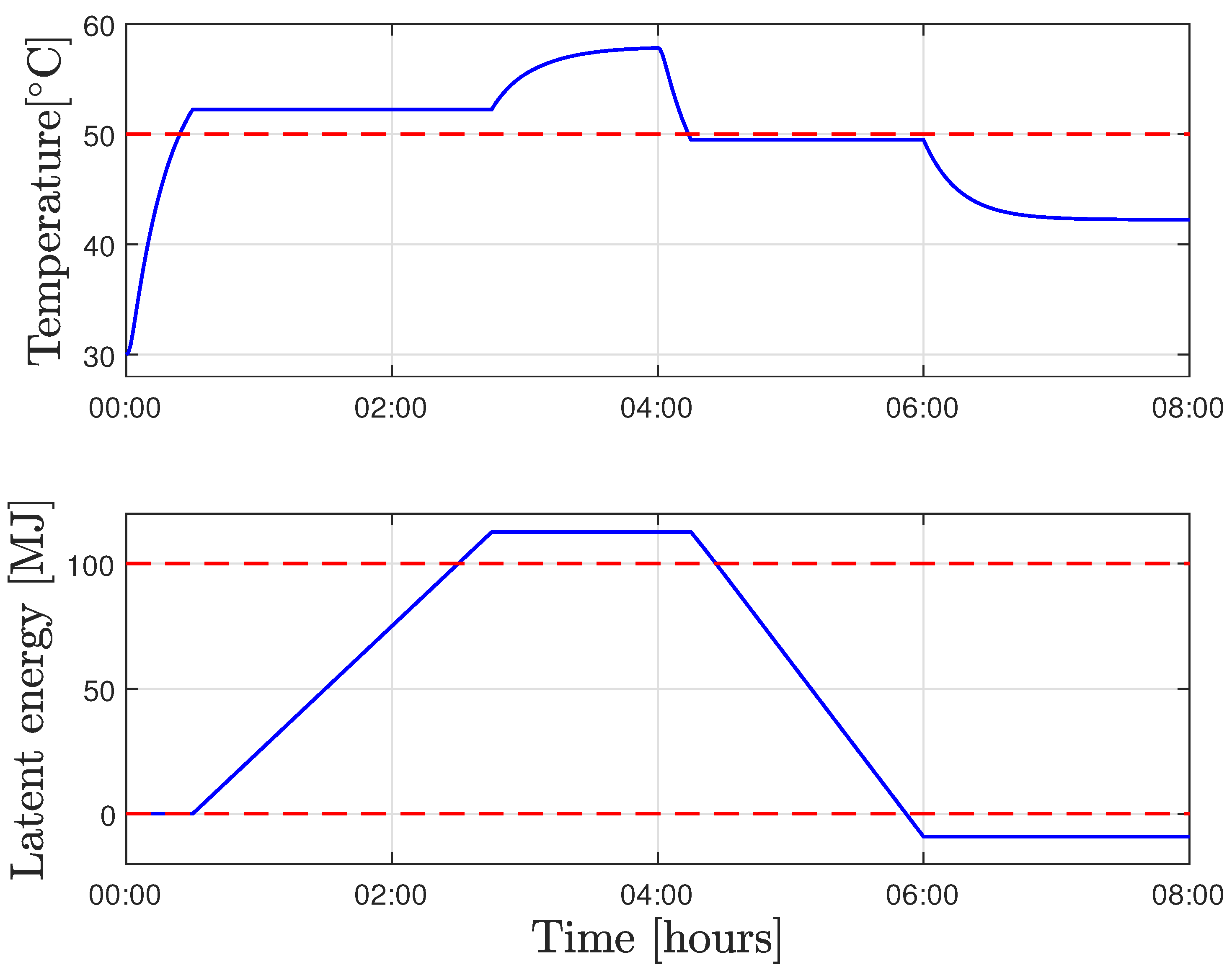
2.5. Model Simulation Results

In this section, the simulations results of the proposed model are presented, which are comparable to the simulations results of the stratified model from Figure 2. Figure 4 shows that the phase change occurs exactly at the demanded temperature, which is fixed at 50 ${}^{\circ }\mathrm{C}$ in this case. Moreover, the latent energy never exceeds the predefined limits of 0 $\mathrm{MJ}$ and 100 $\mathrm{MJ}$ in this example. The simulation of the model is executed in the discrete domain. The model simulation is executed in the discrete domain because the PCM dynamics include discrete steps. This also makes it suitable for a discrete controller design, such as MPC.

3. Model Predictive Control

In this section, the derived model is utilized for MPC. The conditions and limitations related to the heating systems are described, and detailed expressions of implementing all control rules are provided. The optimization problem construction is implemented in Matlab, and it is solved by using the IBM ILOG CPLEX solver [38]. Considering the availability of a computer with a i7 processor and 16 GB RAM, the time to solve the optimization problem for one step is around 20 s. Moreover, the presented simulation of 5 days can be executed within 3 h. During the process of optimization, less than 2 GB of memory is used.

3.1. Model Dimensions

The prediction horizon defines the problem dimension, which has to be considered carefully for the mixed-integer problem. The optimization vector includes continuous state variables, continuous input variables, integer input variables, integer and continuous variables regarding the PCM dynamics and also some other auxiliary variables. There are three continuous state variables (temperature of water, temperature of PCM and energy of PCM) and two input variables (geothermal power and oil boiler power). Moreover, the initial values of water temperature, PCM temperature and PCM energy are optimized. The input variables consist of a continuous value and integer state (ON/OFF). Furthermore, if the heat exchanger allows systems to buy and sell energy with a geothermal source, then one more auxiliary integer variable describes the energy direction and two more auxiliary continuous variables represent the geothermal source limits. The PCM dynamics are described via 4 integer variables (${\delta }_1$, ${\delta }_2$, ${\delta }_3$ and ${\delta }_4$) and 12 continuous variables ($z_{T1}\dots z_{T6}$ and $z_{E1}\dots z_{E6}$), explained in the previous section. Overall, the optimization problem consists of $19N+3$ continuous variables and $7N$ binary variables. Model Equations (28)–(30) are written via MPC equalities, while the explained PCM dynamics along with the temperature and power limitations are written inside the MPC inequalities and bounds.

3.2. Model Variables Substitution and Dimension Reduction

Variable substitution includes expanding the variables to the time horizon. All state variable expressions at any moment can be written by using only the initial state variable and all previous input variables. The temperature of the water at moment k can be expressed by

$$\begin{array}{cc}\hfill T_w\left(k\right)=& A_1^{k-1}[A_1{T}_w\left(0\right)+A_2{T}_{pcm}\left(0\right)]+\hfill \\ & \sum _{i=1}^{k-1}{A}_1^{k-1-i}{A}_2\sum _{j=1}^6{z}_{Tj}\left(i\right)+\sum _{i=0}^{k-1}{A}_1^{k-1-i}B{P}_{gt}\left(i\right)\hfill \\ & +\sum _{i=0}^{k-1}{A}_1^{k-1-i}B{P}_{bo}\left(i\right)-\sum _{i=0}^{k-1}{A}_1^{k-1-i}B{P}_{dem}\left(i\right)\hfill \\ & +\sum _{i=0}^{k-1}{A}_1^{k-1-i}D{T}_{env}\left(i\right).\hfill \end{array}$$

(31)

Furthermore, continuous state variables are removed from the optimization vector. Finally, optimization vector size L is equal to L = 23N + 3.

3.3. Temperature and Power Limitations

The main restriction of a heating system is put on the water temperature. The temperature of the water in storage, i.e., the temperature of the water delivered to the consumers, is needed to respect those limits written into the lower and upper bounds:

$$\begin{array}{c}\hfill lb\le T_w\le ub,\end{array}$$

(32)

where the lower bound ($lb$) is 46 ${}^{\circ }\mathrm{C}$ and the upper bound ($ub$) is 90 ${}^{\circ }\mathrm{C}$ in our case study.

In some cases, the heat exchanger can provide bidirectional energy exchange, so the thermal system is able to sell energy back to the grid. The maximal and minimal geothermal power are regulated by using bounds, where $P_{gt,min}$ [$\mathrm{W}$] is zero in one directional exchange (our case) or a negative number in the case with bidirectional exchange. The $P_{gt,max}$ [$\mathrm{W}$] should always be a positive number, so it follows

$$\begin{array}{c}\hfill P_{gt,min}\le P_{gt}\le P_{gt,max}.\end{array}$$

(33)

The availability of a geothermal source is determined by integer variable ${\delta }_{gt}$, which represents the ON/OFF state of the exchanger, and also by the variable ${\delta }_{grid}$, which shows the relation between the temperature of the storage water and geothermal water ($T_{gt}$ [${}^{\circ }\mathrm{C}$]). The geothermal water needs to be hotter than the water in the bottom of the storage. $\Delta$ is the assumed or measured difference between the storage water of the central part and bottom part of a tank, and is 1 ${}^{\circ }\mathrm{C}$:

$$\begin{array}{c}\hfill (T_w-\Delta )\le T_{gt}\Rightarrow {\delta }_{grid}=1,\end{array}$$

(34)

$$\begin{array}{c}\hfill (T_w-\Delta )>T_{gt}\Rightarrow {\delta }_{grid}=0.\end{array}$$

(35)

Furthermore, the geothermal power sometimes cannot achieve the maximal value due to the small difference between $T_{gt}$ and $T_w$ or low $q_{gt}$. Moreover, when the temperature of the bottom water is higher than the geothermal temperature, then the upper boundary of the geothermal power ($P_{gt}^{+}$ [$\mathrm{W}$]) is zero:

$$\begin{array}{c}\hfill \mathrm{IF}{\delta }_{gt}=1\mathrm{AND}{\delta }_{grid}=1\end{array}$$

$$\begin{array}{cc}\hfill \mathrm{THEN}& P_{gt}^{+}=(T_{gt}-(T_w-\Delta ))c_w{q}_{gt}\hfill \end{array}$$

$$\begin{array}{cc}\hfill \mathrm{ELSE}& P_{gt}^{+}=0\hfill \end{array}$$

Also, when the temperature of the bottom water is higher than the geothermal temperature, the lower boundary of the geothermal power ($P_{gt}^{-}$ [$\mathrm{W}$]) is negative, and the reverse energy transfer to the grid is enabled. However, when $T_{gt}$ is higher than the bottom of the tank, $P_{gt}^{-}$ is zero:

$$\begin{array}{c}\hfill \mathrm{IF}{\delta }_{gt}=1\mathrm{AND}{\delta }_{grid}=0\end{array}$$

$$\begin{array}{cc}\hfill \mathrm{THEN}& P_{gt}^{-}=(T_{gt}-(T_w-\Delta ))c_w{q}_{gt}\hfill \end{array}$$

$$\begin{array}{cc}\hfill \mathrm{ELSE}& P_{gt}^{-}=0\hfill \end{array}$$

The oil boiler model also contains integer variable ${\delta }_b$ representing the ON/OFF state. The limits of the oil power are given with $P_b^{+}$ [$\mathrm{W}$] and $P_b^{-}$ [$\mathrm{W}$]. If $P_b^{-}$ is higher than zero, like in our case, the oil boiler can be considered a disjunctive power source. The following constraints are given:

$$\begin{array}{c}\hfill P_{bo}\le {\delta }_{bo}{P}_{bo}^{+},{\delta }_{bo}{P}_{bo}^{-}\le P_{bo}.\end{array}$$

(36)

3.4. Control Criterion

The control criterion is based on economical profit, whose goal is to minimize energy consumption in monetary terms. The cost function is a linear function given by

$$\begin{array}{c}\hfill J=\sum _{k=0}^N{c}_{gt}\left(k\right)P_{gt}\left(k\right)T_s+\sum _{k=1}^N{c}_{bo}\left(k\right)P_{bo}\left(k\right)T_s,\end{array}$$

(37)

where $c_{gt}$ [$\mathrm{EUR}$/$\mathrm{W}$] and $c_{bo}$ [$\mathrm{EUR}$/$\mathrm{W}$] are price profiles for geothermal energy and oil boiler energy, respectively. The goal of the control algorithm is to use geothermal power as much as possible because it is more affordable but also to maximize energy savings and thus lead to economic benefit.

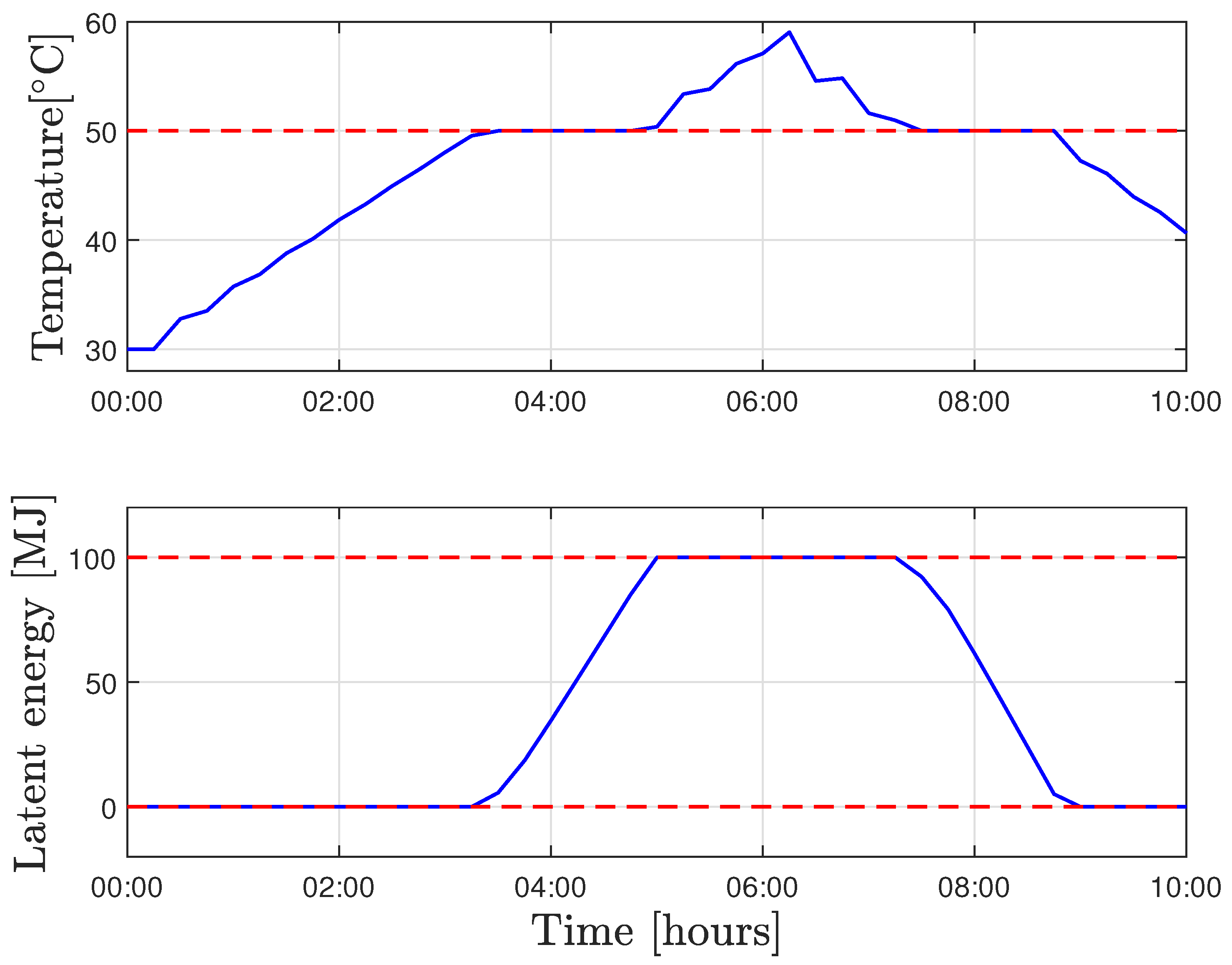
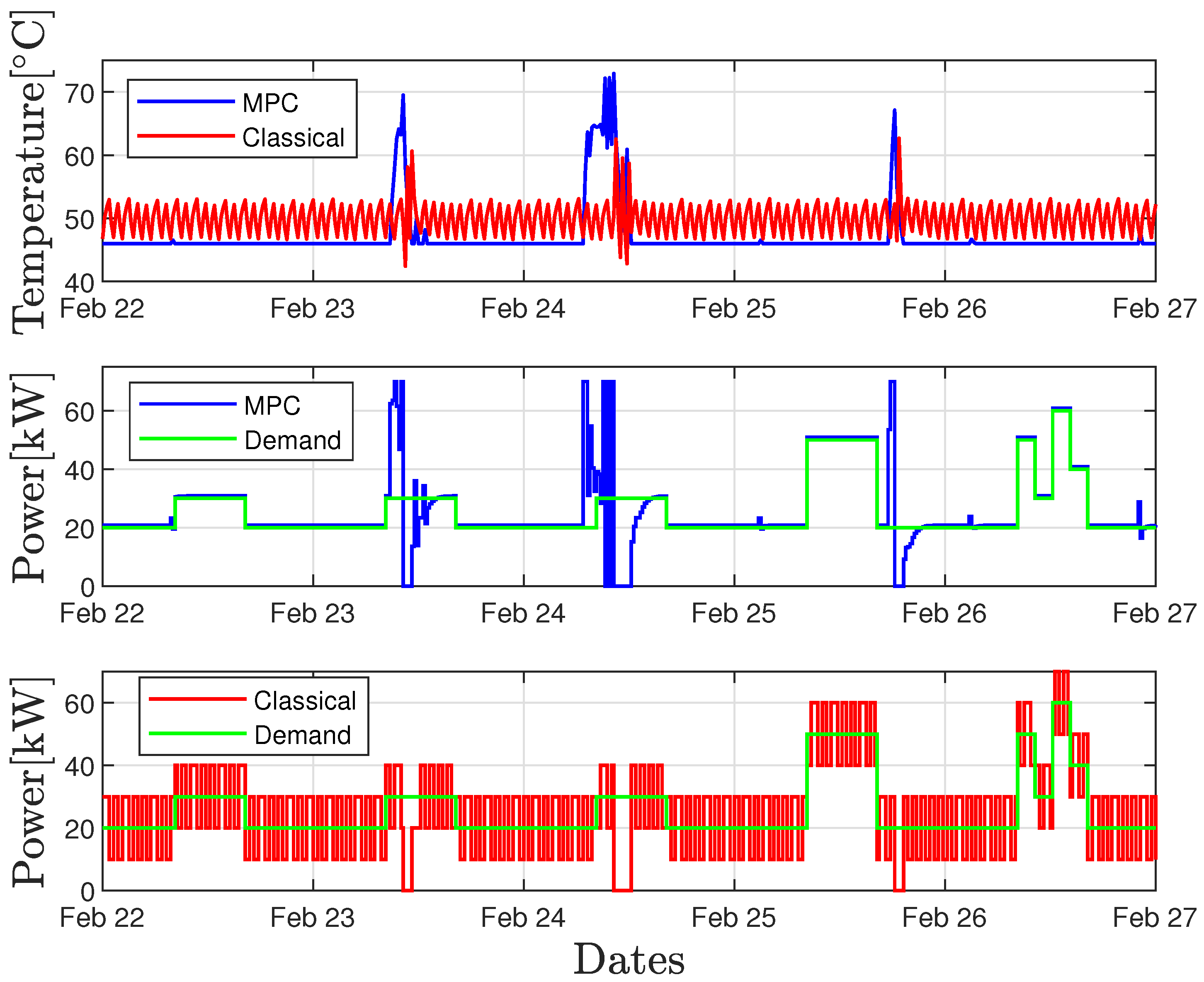
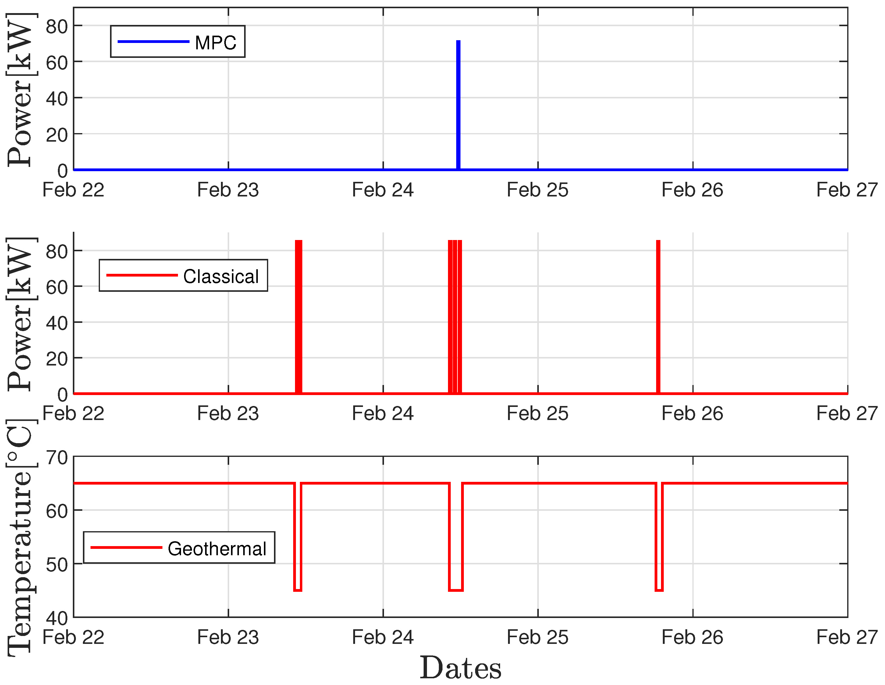
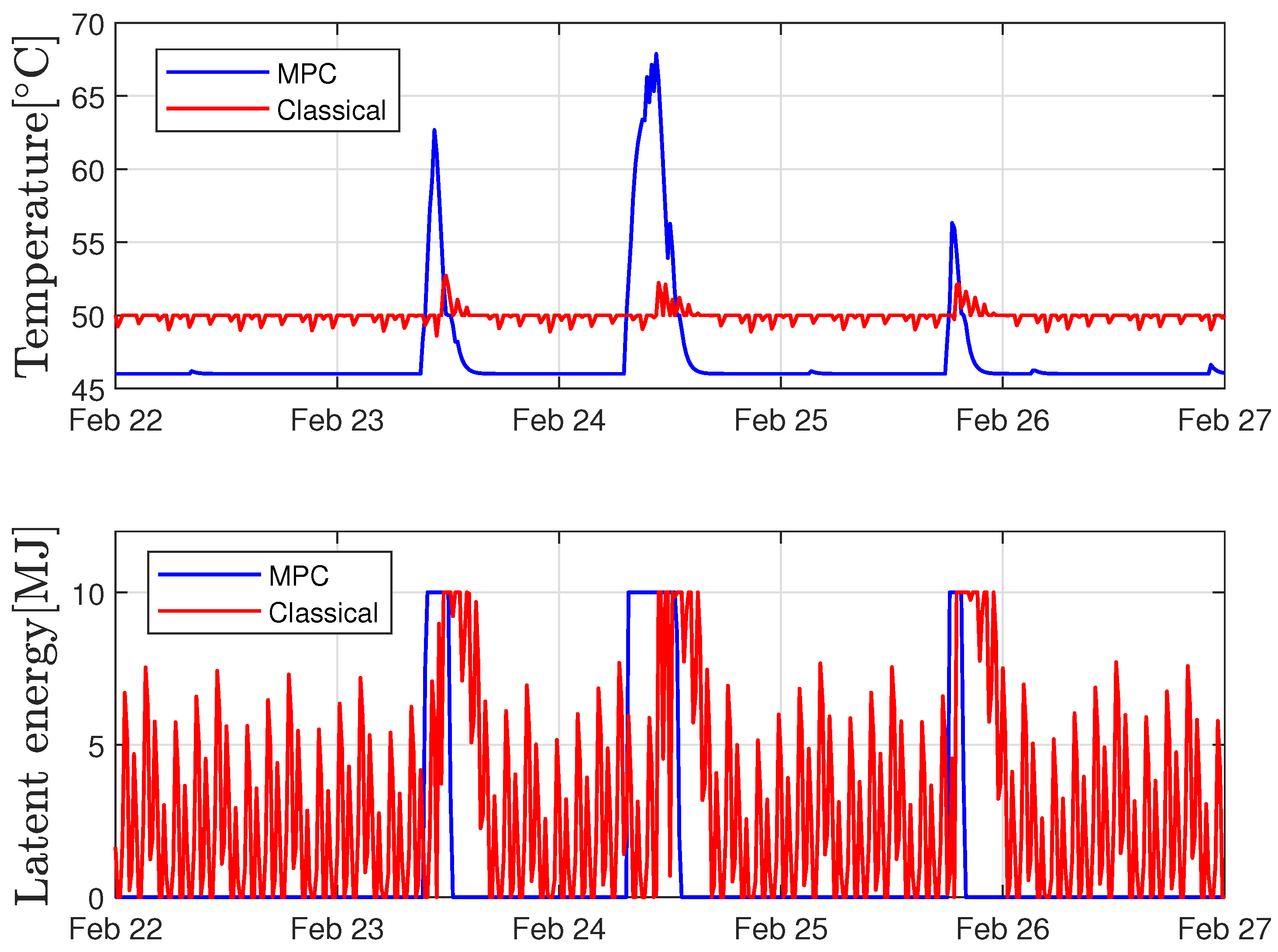
4. Results

4.1. Rule-Based Controller

Hysteresis control is implemented as one type of classical control, so comparison with MPC can be conducted. Hysteresis control is based on IF-THEN-ELSE rules, in which the decision of the input powers is made only by using immediate values of the storage water temperature, geothermal temperature and power demand. Furthermore, the hysteresis controller is given:

1.

IF $T_w<48{}^{\circ }\mathrm{C}$:

(a)

IF ${\delta }_g=1\Rightarrow P_{gt}=P_{dem}+10,P_{bo}=0$

(b)

IF ${\delta }_g=0\Rightarrow P_{gt}=0,P_{bo}=P_{bo}^{+}$

2.

IF $T_w>52{}^{\circ }\mathrm{C}$:

(a)

IF ${\delta }_g=1\Rightarrow P_{gt}=P_{dem}-10,P_{bo}=0$

(b)

IF ${\delta }_g=0\Rightarrow P_{gt}=0,P_{bo}=0$

Goal of the control is to keep the water temperature between 48 ${}^{\circ }\mathrm{C}$ and 52 ${}^{\circ }\mathrm{C}$. If the temperature drops below 48 ${}^{\circ }\mathrm{C}$, if possible, the system is then using the geothermal source with 10 $\mathrm{W}$ additional power than power demand. On the other hand, if the temperature exceeds 52 ${}^{\circ }\mathrm{C}$, the geothermal source with 10 $\mathrm{W}$ less power than the power demand is used, if possible. It is expected that the temperature will stay above the lower bound of 46 ${}^{\circ }\mathrm{C}$ and that energy efficiency will be achieved by avoiding using an oil boiler whenever it is possible.

4.2. MPC Parameters

A discrete time step of 15 min is chosen as a trade-off between accuracy in capturing the thermal dynamics and the dimensionality of the problem such that the problem can be solved within the time step. A time horizon of 6 h is used, meaning that 24 steps in advance are taken into account. The geothermal power is limited between 0 $\mathrm{kW}$ and 70 $\mathrm{kW}$. Selling energy back to the grid is not possible for the considered case study. The oil boiler is a disjunctive power source, being within the limits of 71 $\mathrm{kW}$ and 85 $\mathrm{kW}$ when it is on. The oil boiler energy price is about four times bigger than the price for energy from a geothermal source (0.0828 [$\mathrm{EUR}/\mathrm{kWh}$] to 0.0229 [$\mathrm{EUR}/\mathrm{kWh}$]). The minimal temperature of the supplied water is set to be 46 ${}^{\circ }\mathrm{C}$, and going below this limit violates user comfort. The PCM temperature of change is 50 ${}^{\circ }\mathrm{C}$, while the maximal latent energy is 10 $\mathrm{MJ}$.

4.3. Simulations

Both control algorithms are tested and compared on 5 days of simulations from the 22nd of February to the 27th of February in 2023. Each day between 00:00–08:00 and 16:00–24:00 are non-working hours, and power demand is 20 $\mathrm{kW}$. In first three days during working hours, that is, 08:00–16:00, the power demand is 30 $\mathrm{kW}$, which can be seen in Figure 5 with the green line. During the fourth day, the power demand is 50 $\mathrm{kW}$, and during the fifth day, it is changeable. In the second graph in Figure 5, it can be seen that MPC uses a geothermal source to follow the power demand by using prediction, and the best tracking is shown on day 5. On the other hand, the classical controller uses the geothermal source in an oscillatory way as it is seen in the third graph in Figure 5, which leads to a shorter life span of the system components due to the frequent ON/OFF switching of the valves and the changing water flow. In the first graph in Figure 5, it is shown that MPC satisfies the temperature constraint by always keeping the water temperature above the minimum of 46 ${}^{\circ }\mathrm{C}$. On the other hand, as it is shown in first graph in Figure 5, the classical control violates the constraint in periods with low geothermal temperature. Due to the lower geothermal temperature, in some periods that are shown in the third graph in Figure 6, the geothermal source is unavailable. MPC anticipates this by using a higher level of the geothermal source one step before. After that, MPC immediately uses all the stored latent energy, while the classical controller is not able to because it does not contain the variable of latent energy in its algorithm as it is presented in Figure 7. In addition, MPC does not use the oil boiler power at all on 23 February and 25 February. However, on the 24 February, the period of geothermal source unavailability is longer, so MPC needs to use the oil boiler power but with a lower amount than classical control as it is shown in Figure 6.

The economical benefit of applying the MPC in the considered scenario of five days shows that MPC spent EUR 74.20, while classical control spent 81.03 EUR. The monetary savings of 8.43% are achieved. Moreover, MPC contributes to switching ON/OFF units and changing the power amounts significantly fewer times, which significantly prolongs the system life span. In this scenario, classical control changes the geothermal source power level 4 times more than MPC (219 times by classical approach compared to 50 times by MPC during 5 days). In addition, whenever the geothermal source becomes unavailable, the classical control disregards user comfort by letting the temperature of water that is delivered to the consumers, to drop more than 3 ${}^{\circ }\mathrm{C}$ below minimal requested level. MPC satisfies user needs and keeps the water temperature at the desired level. Furthermore, MPC tracks the optimal water temperature, i.e., 46 ${}^{\circ }\mathrm{C}$, better than the classical control, which leads to lower mean absolute error (MAE is 1.06 ${}^{\circ }\mathrm{C}$ by MPC compared to 3.98 ${}^{\circ }\mathrm{C}$ by classical control).

5. Conclusions

This paper proposes a mathematical model and optimal control strategy for latent heat storage. A low-order mixed logical dynamical (MLD) mathematical model is derived that is fast to execute due to its simplicity and is suitable for optimal control, such as MPC. The dynamics of PCM takes future states into account, which leads to high accuracy of the proposed model, regarding both temperature and latent energy. Results show that the proposed control algorithm achieves better user satisfaction compared to classical rule-based control. Moreover, it extends the thermal system equipment life span, while also acquiring lower economic costs. Furthermore, significant savings of the heating system operational costs are achieved when the derived control performance is compared with a classical rule-based control.

References

- Copernicus: 2022 Was a Year of Climate Extremes, with Record High Temperatures and Rising Concentrations of Greenhouse Gases. European Centre for Medium-Range Weather Forecasts. 2022. Available online: https://climate.copernicus.eu/copernicus-2022-was-year-climate-extremes-record-high-temperatures-and-rising-concentrations (accessed on 22 August 2023).
- EU Economy Greenhouse Gas Emissions in Q2 2022. Eurostat. 2022. Available online: https://ec.europa.eu/eurostat/web/products-eurostat-news/-/ddn-20221115-2 (accessed on 22 August 2023).
- Greenhouse Gas Emissions from Energy Use in Buildings in Europe; European Environment Agency: Copenhagen, Denmark, 2021. Available online: https://www.eea.europa.eu/ims/greenhouse-gas-emissions-from-energy (accessed on 22 August 2023).
- ’Fit for 55’: Delivering the EU’s 2030 Climate Target on the Way to Climate Neutrality; European Commission: Brussels, Belgium, 2021. Available online: https://www.fao.org/faolex/results/details/en/c/LEX-FAOC211249/ (accessed on 22 August 2023).
- Quadrennial Technology Review 2015: “Chapter 5—Increasing Efficiency of Buildings Systems and Technologies Department of Energy”. 2015. Available online: https://www.energy.gov/sites/prod/files/2017/03/f34/qtr-2015-chapter5.pdf (accessed on 22 August 2023).
- Pielichowska, K.; Pielichowski, K. Phase change materials for thermal energy storage. Prog. Mater. Sci. 2014, 65, 67–123. [Google Scholar] [CrossRef]
- Sharma, A.; Tyagi, V.V.; Chen, C.R.; Buddhi, D. Review on thermal energy storage with phase change materials and applications. Renew. Sustain. Energy Rev. 2007, 13, 318–345. [Google Scholar] [CrossRef]
- Teamah, H.M. Comprehensive review of the application of phase change materials in residential heating applications. Alex. Eng. J. 2021, 60, 3829–3843. [Google Scholar] [CrossRef]
- Kuznik, F.; David, D.; Johannes, K.; Roux, J.J. A review on phase change materials integrated in building walls. Renew. Sustain. Energy Rev. 2011, 15, 379–391. [Google Scholar] [CrossRef]
- Reddy, R.M.; Nallusamy, N.; Reddy, K.H. Experimental Studies on Phase Change Material-Based Thermal Energy Storage System for Solar Water Heating Applications. J. Fundam. Renew. Energy Appl. 2012, 2, R120314. [Google Scholar] [CrossRef]
- Li, B.; Zhai, X.; Cheng, X. Experimental and numerical investigation of a solar collector/storage system with composite phase change materials. Sol. Energy 2018, 164, 2018. [Google Scholar] [CrossRef]
- Stutz, B.; Le Pierres, N.; Kuznik, F.; Johannes, K.; Del Barrio, E.P.; Bedecarrats, J.P.; Gibout, S.; Marty, P.; Zalewski, L.; Soto, J.; et al. Storage of thermal solar energy. Comptes Rendus Phys. 2017, 18, 401–414. [Google Scholar] [CrossRef]
- Mazzoni, S.; Sze, J.Y.; Nastasi, B.; Ooi, S.; Desideri, U.; Romagnoli, A. A techno-economic assessment on the adoption of latent heat thermal energy storage systems for district cooling optimal dispatch and operations. Appl. Energy 2021, 289, 116646. [Google Scholar] [CrossRef]
- Baek, S.; Kim, S. Analysis of Thermal Performance and Energy Saving Potential by PCM Radiant Floor Heating System based on Wet Construction Method and Hot Water. Energies 2019, 12, 828. [Google Scholar] [CrossRef]
- Hofmann, R.; Dusek, S.; Gruber, S.; Drexler-Schmid, G. Design Optimization of a Hybrid Steam-PCM Thermal Energy Storage for Industrial Applications. Energies 2019, 12, 898. [Google Scholar] [CrossRef]
- Touretzky, C.R.; Salliot, A.A.; Lefevre, L.; Baldea, M. Optimal Operation of Phase-Change Thermal Energy Storage for a Commercial Building. In Proceedings of the American Control Conference, Chicago, IL, USA, 1–3 July 2015; pp. 980–985. Available online: https://www.researchgate.net/publication/282826606_Optimal_operation_of_phase-change_thermal_energy_storage_for_a_commercial_building (accessed on 22 August 2023).
- Mohamed, H.; Brahim, A.B. Modeling and dynamic simulation of a thermal energy storage system by sensitive heat and latent heat. In Proceedings of the International Conference on Green Energy Conversion Systems (GECS), Hammamet, Tunisia, 23–25 March 2017; pp. 1–7. Available online: https://www.researchgate.net/publication/320603688_Modeling_and_dynamic_simulation_of_a_thermal_energy_storage_system_by_sensitive_heat_and_latent_heat (accessed on 22 August 2023).
- Mekaddem, N.; Ali, S.B.; Hannachi, A.; Mazioud, A.; Foi, M. Latent energy storage study in simple and honeycomb structures filled with a phase change material. In Proceedings of the 2016 7th International Renewable Energy Congress (IREC), Hammamet, Tunisia, 22–24 March 2016; pp. 1–6. Available online: https://ieeexplore.ieee.org/abstract/document/7478884 (accessed on 22 August 2023).
- Shanks, M.; Jain, N. Control of a Hybrid Thermal Management System: A Heuristic Strategy for Charging and Discharging a Latent Thermal Energy Storage Device. In Proceedings of the 2022 21st IEEE Intersociety Conference on Thermal and Thermomechanical Phenomena in Electronic Systems (iTherm), San Diego, CA, USA, 31 May–3 June 2022; pp. 1–10. Available online: https://ieeexplore.ieee.org/document/9899546 (accessed on 22 August 2023).
- Yang, S.; Gao, H.O.; You, F. Model Predictive Control for Price-Based Demand-Responsive Building Control by Leveraging Active Latent Heat Storage. In Proceedings of the 2022 IEEE 61st Conference on Decision and Control (CDC), Cancun, Mexico, 6–9 December 2022; pp. 539–544. [Google Scholar] [CrossRef]
- Chuttar, A.; Shettigar, N.; Thyagrajan, A.; Banerjee, D. Deep Learning to Enhance Transient Thermal Performance and Real-Time Control of an Energy Storage (TES) Platform. In Proceedings of the 2021 20th IEEE Intersociety Conference on Thermal and Thermomechanical Phenomena in Electronic Systems (iTherm), San Diego, CA, USA, 1–4 June 2021; pp. 1036–1044. [Google Scholar] [CrossRef]
- Dermardiros, V.; Chen, Y.; Athienitis, A.K. Modelling of an Active PCM Thermal Energy Storage for Control Applications. Energy Procedia 2015, 78, 1690–1695. [Google Scholar] [CrossRef]
- Vrbanc, F.; Rukavina, F.; Lešić, V.; Vašak, M. Mixed Logical Dynamical Modelling of a Stratified Storage with Phase-Change Material. IFAC-PapersOnLine 2022, 55, 145–150. [Google Scholar] [CrossRef]
- Gholamibozanjani, G.; Farid, M. Application of an active PCM storage system into a building for heating/cooling load reduction. Energy 2020, 210, 118572. [Google Scholar] [CrossRef]
- Pangborn, H.C.; Laird, C.E.; Alleyne, A.G. Hierarchical Hybrid MPC for Management of Distributed Phase Change Thermal Energy Storage. In Proceedings of the 2020 American Control Conference (ACC), Denver, CO, USA, 1–3 July 2020; pp. 4147–4153. [Google Scholar] [CrossRef]
- Buerger, A.; Bohlayer, M.; Hoffmann, S.; Altmann-Dieses, A.; Braun, M.; Diehl, M. A whole-year simulation study on nonlinear mixed-integer model predictive control for a thermal energy supply system with multi-use components. Appl. Energy 2020, 258, 114064. [Google Scholar] [CrossRef]
- Rafii-Tabrizi, S.; Hadji-Minaglou, J.-R.; Scholzen, F. Mixed Integer Linear Programming Model for the Optimal Operation of a Dual Source Heat Pump. In Proceedings of the 2019 6th International Conference on Control, Decision and Information Technologies (CoDIT), Paris, France, 23–26 April 2019; pp. 373–378. [Google Scholar] [CrossRef]
- Verrilli, F.; Srinivasan, S.; Gambino, G.; Canelli, M.; Himanka, M.; Del Vecchio, C.; Sasso, M.; Glielmo, L. Model Predictive Control-Based Optimal Operations of District Heating System With Thermal Energy Storage and Flexible Loads. IEEE Trans. Autom. Sci. Eng. 2017, 14, 547–557. [Google Scholar] [CrossRef]
- Dorfner, J.; Hamacher, T. Large-Scale District Heating Network Optimization. IEEE Trans. Smart Grid 2014, 5, 1884–1891. [Google Scholar] [CrossRef]
- Risbeck, M.J.; Maravelias, C.T.; Rawlings, J.B.; Turney, R.D. Cost optimization of combined building heating/cooling equipment via mixed-integer linear programming. In Proceedings of the 2015 American Control Conference (ACC), Chicago, IL, USA, 1–3 July 2015; pp. 1689–1694. [Google Scholar] [CrossRef]
- Rukavina, F.; Vašak, M. Mixed-integer Modelling and Optimization of a Heat Source and a Storage System. IFAC-PapersOnLine 2022, 55, 133–138. [Google Scholar] [CrossRef]
- Deng, K.; Sun, Y.; Li, S.; Lu, Y.; Brouwer, J.; Mehta, P.G.; Zhou, M.; Chakraborty, A. Model Predictive Control of Central Chiller Plant With Thermal Energy Storage Via Dynamic Programming and Mixed-Integer Linear Programming. IEEE Trans. Autom. Sci. Eng. 2015, 12, 565–579. [Google Scholar] [CrossRef]
- Candanedo, J.A.; Dehkordi, V.R.; Stylianou, M. Model-based predictive control of an ice storage device in a building cooling system. Appl. Energy 2013, 111, 1032–1045. [Google Scholar] [CrossRef]
- Heine, K.; Tabares-Velasco, P.C.; Deru, M. Design and dispatch optimization of packaged ice storage systems within a connected community. Appl. Energy 2021, 298, 117147. [Google Scholar] [CrossRef]
- Zhang, D.; Shah, N.; Papageorgiou, L.G. Efficient energy consumption and operation management in a smart building with microgrid. Energy Convers. Manag. 2013, 74, 209–222. [Google Scholar] [CrossRef]
- Lu, Y.; Wang, S.; Sun, Y.; Yan, C. Optimal scheduling of buildings with energy generation and thermal energy storage under dynamic electricity pricing using mixed-integer nonlinear programming. Appl. Energy 2015, 147, 49–58. [Google Scholar] [CrossRef]
- Bemporad, A.; Morari, M. Control of systems integrating logic, dynamics, and constraints. Automatica 1999, 35, 407–427. [Google Scholar] [CrossRef]
- BM ILOG CPLEX. Optimization Studio Getting Started with CPLEX for MATLAB. Available online: https://www.ibm.com/docs/es/icos/22.1.0?topic=SSSA5P_22.1.0/ilog.odms.studio.help/Optimization_Studio/topics/COS_home.html (accessed on 22 August 2023).
Disclaimer/Publisher’s Note: The statements, opinions and data contained in all publications are solely those of the individual author(s) and contributor(s) and not of MDPI and/or the editor(s). MDPI and/or the editor(s) disclaim responsibility for any injury to people or property resulting from any ideas, methods, instructions or products referred to in the content. |
© 2023 by the authors. Licensee MDPI, Basel, Switzerland. This article is an open access article distributed under the terms and conditions of the Creative Commons Attribution (CC BY) license (https://creativecommons.org/licenses/by/4.0/).
Share and Cite
Vrbanc, F.; Vašak, M.; Lešić, V. Simple and Accurate Model of Thermal Storage with Phase Change Material Tailored for Model Predictive Control. Energies 2023, 16, 6849. https://doi.org/10.3390/en16196849
Vrbanc F, Vašak M, Lešić V. Simple and Accurate Model of Thermal Storage with Phase Change Material Tailored for Model Predictive Control. Energies. 2023; 16(19):6849. https://doi.org/10.3390/en16196849
Chicago/Turabian StyleVrbanc, Filip, Mario Vašak, and Vinko Lešić. 2023. "Simple and Accurate Model of Thermal Storage with Phase Change Material Tailored for Model Predictive Control" Energies 16, no. 19: 6849. https://doi.org/10.3390/en16196849
APA StyleVrbanc, F., Vašak, M., & Lešić, V. (2023). Simple and Accurate Model of Thermal Storage with Phase Change Material Tailored for Model Predictive Control. Energies, 16(19), 6849. https://doi.org/10.3390/en16196849