Article

Investigation of the Performance of Thermodynamic Analysis Models for a Cryocooler PPG-102 Stirling Engine

by
George Antonakos
,
Irene Koronaki
*,
George-Rafael Domenikos
and
Serafeim Baltadouros
Laboratory of Applied Thermodynamics, Mechanical Engineering School, National Technical University of Athens, Zografou Campus, Heroon Polytecheiou 9, 15780 Athens, Greece
*
Author to whom correspondence should be addressed.
Energies 2023, 16(19), 6815; https://doi.org/10.3390/en16196815
Submission received: 9 August 2023 / Revised: 6 September 2023 / Accepted: 18 September 2023 / Published: 26 September 2023
(This article belongs to the Section J1: Heat and Mass Transfer)

Abstract

:
Three distinct thermodynamic analysis models are developed and applied to a renowned cryogenic engine (PPG-102), namely the isothermal model, the ideal Schmidt model, and the ideal adiabatic model. Through a comparative analysis, the theoretical outcomes derived from these models are juxtaposed with the corresponding theoretical results from the existing literature. The comprehensive evaluation of these findings demonstrates significant convergence, with minor deviations primarily attributed to the inherent assumptions underlying each model. The design of the PPG-102 engine is meticulously executed within the Solidworks environment, allowing for the subsequent simulation under operating conditions identical to those of the computational models. Remarkably, the simulation results closely approximate the outcomes of the adiabatic analysis, thus corroborating the validity and effectiveness of this particular model. In this work, the presented models, initially developed for thermal Stirling engines, are augmented and applied to a cryogenics Stirling engine, offering a unique understanding of the workings of this apparatus.

1. Introduction

A Stirling engine functions based on a thermodynamic regenerative cycle that operates in a closed system. The engine utilizes a single working fluid, which undergoes repeated compression and expansion stages at various temperature levels, resulting in a net conversion of heat into work, or vice versa. This versatile engine has applications as a cooling device, a primary driving mechanism, a heat pump, and even a pressure generator [1,2,3]. Alexander Kirk, a Scottish engineer employed at the oil works in Bathgate, Scotland, played a significant role in the development of the first Stirling cooling engines. He successfully constructed cooling engines for various purposes, both within Great Britain and internationally. Notably, Kirk is credited with pioneering the cascade cycle, which has since become widely employed in cryogenic applications and the liquefaction and processing of low-temperature gases. Collins (1958) [4] recognized Kirk as a noteworthy figure, acknowledging his prowess not only as a skilled machine designer but also as a scientific thinker. Despite these achievements, the Kirk machines were not produced in large quantities or utilized to achieve cryogenic temperatures. In around 1946, a significant milestone in the advancement of Stirling cooling engines took place with the commencement of Philips’ research on the subject. This initiative followed a decade of dedicated work focused on small Stirling engine prime movers. It was during the early 1950s that Stirling engines began to be acknowledged and categorized as a distinct and specific class of machinery. Since then, the term “Stirling engine” has gained widespread acceptance as the generic name for closed-cycle regenerative thermal systems, regardless of whether they are utilized as prime movers or cooling engines. This approach is preferred over the practice employed by some individuals who refer to the Kirk cycle when describing Stirling engines operating as refrigerators. It is important to distinguish between the two main classes of regenerative machines: Stirling engines (without valves) and Ericsson engines (with valves). This classification is based on whether the control of internal fluid flows is achieved through changes in volume or through the use of valves. The pioneering company Philips has manufactured several refrigeration systems, including the B-type cryocooler PPG-102. Martini proposed a second-order analysis method for Stirling thermal machines in 1978 [5]. Four years later, he also suggested a second-order analysis technique for Stirling cryocoolers [6]. The PPG-102 liquefier was subjected to second-order analysis in 1989 by Walker, Weiss, Fauvel, and Reader [7], who successfully utilized Martini’s proposed analysis. Furthermore, in 1990, Atrey, Bapat, and Narayankhedkar proposed a cyclic simulation of Stirling cryocoolers, considering the compression process as adiabatic and the expansion process as isothermal [8]. Later, Ruijie Li and Lvinia Grosu [9] developed an isothermal model for analyzing the PPG-102 machine, and their results correlated with the corresponding theoretical results from the literature. In the Appendix A the technical and operational characteristics of the specific cryocooler [10] are presented. In the present study, three different second-order analysis models are presented, as developed in the Laboratory of Applied Thermodynamics at the National Technical University of Athens (NTUA). The models are based on the isothermal and adiabatic models presented by Urieli and Berchowitz [11] and the analysis by Schmidt [12]. A comparison of the results is carried out with the corresponding results from the literature. To validate the thermodynamic analysis models and their results, a three-dimensional model of the PPG-102 cryocooler is developed using Solidworks software. The model is updated with the thermo-physical properties of the materials used in the actual machine, the operating conditions are adjusted, and the boundary and interface conditions under which it is assumed to operate are specified.

2. Thermodynamic Analysis Models

Various models have been developed for the analysis of thermal and cryogenic Stirling engines, each with its own assumptions. Walker et al. [7] utilized the isothermal model for studying thermal and cryogenic Stirling engines. Similarly, the authors utilized an isothermal model in their previous work [13]. Urieli and Berchowitz presented a series of thermodynamic analysis models for Stirling engines. In addition, valuable insights into the 1D and 3D modeling of Stirling engines were gained from the works of Rogdakis et al. [14] and Bitsikas et al. [15]. Based on these models and for the purposes of this work, computational codes are developed for the thermodynamic analysis of cryogenic Stirling engines. Subsequently, a concise yet comprehensive overview of the isothermal analysis models, Schmidt analysis, and ideal adiabatic analysis is provided. The assumptions used in each model are presented, as well as the key energy results they calculate. The obtained results are compared with the corresponding results from the literature.

2.1. Isothermal Analysis

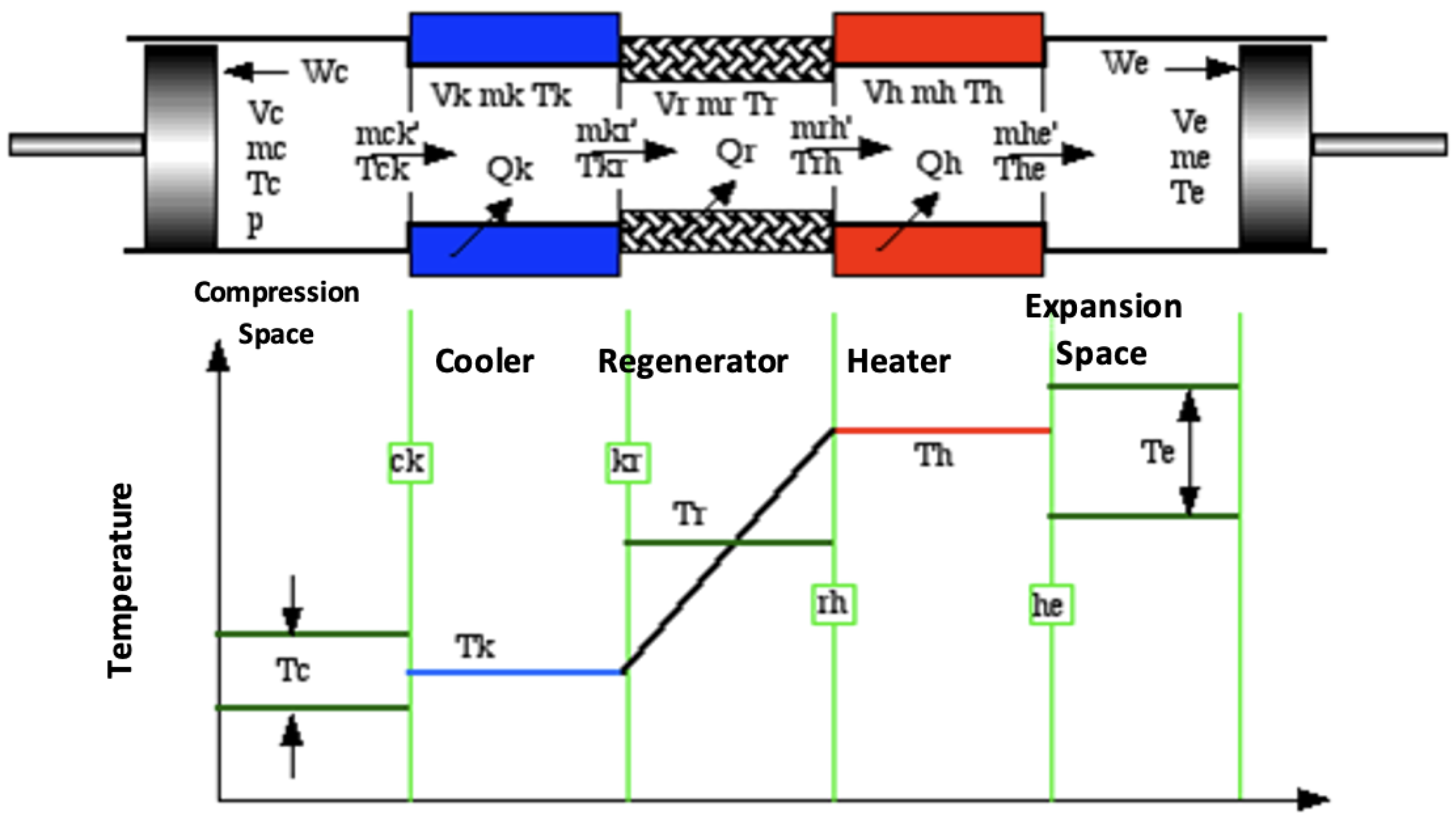
The fundamental assumption of an isothermal analysis is that the working fluid in the expansion space and the heater is at a constant high temperature, whereas in the compression space and the cooler, it is at a constant low temperature. This isothermal approach allows us to express pressure as a function of the volume variation. It also enables the exploration of the impact of the type of kinematic mechanism on the generated power. The assumption of isothermal working spaces and heat exchangers implies that the heat exchangers, including the regenerator, are ideal. The temperature distribution of the machine’s spaces is shown in Figure 1. Each Stirling engine, whether power or cryocooler, consists of five fundamental parts arranged in series (the compression space (c), cooler (k), regenerator (r), heater (h), and freezer if we are talking about cryocoolers) and the expansion space (e). The various connecting passages between these parts are included in the dead space of the compression and expansion spaces. Each space component is considered a homogeneous space or cell, where the gas has a constant mass (m), absolute temperature (T), volume (V), and pressure (p). Specifically, the pressure is assumed to be the same in all spaces of the engine at a given moment. In this ideal case, it is also assumed that there is no pressure drop.
The isothermal analysis model takes into account the following assumptions:
  • The mass of the working fluid is constant, meaning there are no losses.
  • The ideal gas equation holds true.
  • The speed (frequency) of the engine is constant.
  • Cyclical thermodynamic variation.
  • The kinetic and dynamic energy of the gases is neglected.
In an isothermal analysis, the objective is to determine the work produced by the engine and the amount of transferred heat. This is achieved by calculating the area enclosed within the P-V diagram. Initially, we assume that the mass of the working fluid remains constant. Based on the mathematical foundations of the Stirling engines as offered by Urieli et al. [11], the mathematical model that is used is presented in Equations (1)–(23).
M = m c + m k + m r + m h + m e
From the equation of ideal gases, we have:
m = p V R T
Thus,
M = p ( V c T k + V k T k + V r T r + V h T h + V e T h ) R
The average value of pressure per crank angle at a specific moment in time can be calculated as follows:
p = M R ( V c T k + V k T k + V r l n ( T h T k ) T h T k + V h T h + V e T h ) 1
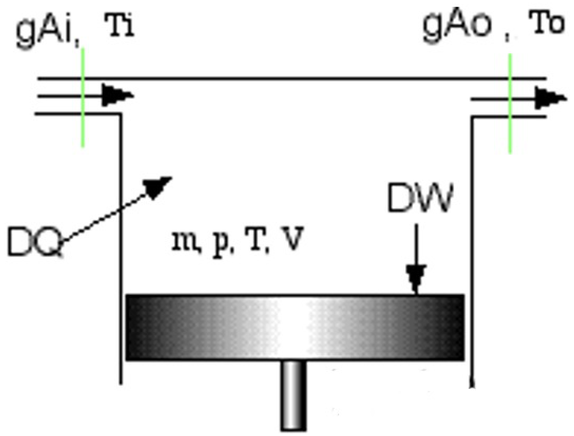
The total required work is obtained by algebraically summing the consumed work and the produced work in the compression and expansion spaces, respectively. A typical cell of a working space is shown in Figure 2. Enthalpy enters the cell space through the mass flow rate g A i and temperature T i and exits through the mass flow rate g A i and temperature T o .
The energy equation for non-steady flow conditions, where kinetic and potential energy can be neglected, is described as follows:
D Q + ( c p T i g A i c p T o g A o ) = D W + c v D m T
In the isothermal model, both in the working spaces (compression and expansion) and the heat exchangers (cooler and heater or freezer), the temperature remains constant: T i = T o = T . Thus,
D Q + c p T ( g A o g A i ) = D W + c v T D m + D W
From the conservation of mass, the difference in the mass flows is seen to be the rate of remaining mass in the cell. Thus, Equation (6) is written as:
D Q = D W + R T D m
where, considering an ideal gas, we have: R = c p c v .
The amount of net transferred heat to the working fluid during each cycle of operation is calculated by integrating Equation (7) along the path. Thus,
Q = D Q = R T D M + D W
In the table below (Table 1), the required equations for the analysis of the isothermal model are summarized. To solve these equations, we need to determine the changes in the volume of the working spaces and their corresponding differentials. These depend on the type of engine (method of piston driving) being used:

2.2. Schmidt Analysis

Most studies that analyze the Stirling thermodynamic cycle have been based on this theory. The original publication of Schmidt’s theory is not available but various translations and interpretations of it exist. Many of these interpretations shed light on the computation of equations corresponding to the isothermal analysis of Stirling engines, especially regarding the consideration of sinusoidal variations in the volumes of the working spaces. The performance of the engine is described by a P-V diagram. The volumes of the different parts of the engine can be easily calculated by studying its internal geometry. Once the volumes, mass of the working gas, and temperatures of the respective spaces are determined, the average pressure can be calculated using the ideal gas equation of state (Equation (4)). The Schmidt analysis is applied to each configuration of Stirling engines, including the PPG-102 engine, which is the subject of this study. The PPG-102 engine belongs to the Beta configuration, where the displacer and compression piston are in the same chamber, whereas the heater, regenerator, and cooler are together in a separate chamber. The equations that describe the volume variations in the engine cylinders are as follows:
V e ( θ ) = V s w e 2 ( 1 c o s ( θ ) ) + V c l e
V c ( θ ) = V s w e 2 ( 1 c o s ( θ ) ) + V s w c 2 ( 1 c o s ( θ d θ ) ) + V c l c V B
At the moment when the strokes of the pistons overlap, an active space with volume VB called the “overlap volume” appears and is calculated using the following formula:
V B = V s w e + V s w c 2 V s w e 2 + V s w c 2 4 V s w e V s w c 2 c o s ( θ ) d θ
Therefore, the total volume is given by the equation:
V ( θ ) = V e ( θ ) + V c ( θ ) + V B
The value of the working fluid pressure, as well as the maximum and minimum values, are obtained from the equation:
p = p m e a n 1 c 2 1 c c o s ( θ α ) = p m i n ( 1 + c ) 1 c c o s ( θ α ) = p m a x ( 1 c ) 1 c c o s ( θ α )
where:
α = a r c t a n ( κ s i n ( θ ) d θ τ + c o s ( θ ) d θ + 1 )
S = τ + 2 τ X e + 4 τ X r 1 + τ + κ + 2 X c + 1 X B
B = τ 2 + 2 ( τ 1 ) κ c o s ( θ ) d θ + κ 2 2 τ + 1
c = B S
In Equation (15), the following ratios were used:
τ = T c T e κ = V s w c V s w e χ B = V B V s w e χ e = V c l e V s w e χ c = V c l c V s w e χ r = V r V s w e
The recommended energy in the expansion space, We, as a function of the mean pressure, p m e a n , as well as the maximum and minimum values, is given by the equation:
W e = p d V e = p m e a n V s w e π c s i n ( α ) 1 + 1 c 2 = p m i n V s w e π c s i n α 1 + 1 c 2 1 + c 1 c = p m a x V s w e π c s i n α 1 + 1 c 2 1 c 1 + c
Similarly, for the consumed work in the compression space, Wc, as a function of the mean pressure, p m e a n , as well as the maximum and minimum values, we have:
W c = p d V c = p m e a n V s w e π c t s i n ( α ) 1 + 1 c 2 = p m i n V s w e π c t s i n α 1 + 1 c 2 1 + c 1 c = p m a x V s w e π c t s i n α 1 + 1 c 2 1 c 1 + c
With the total exchanged work being:
W = W e + W c
The relationships that relate the average pressure p m e a n to the extreme values p m i n and p m a x are given by the equations:
p m i n p m e a n = 1 c 1 + c
and
p m a x p m e a n = 1 + c 1 c
The coefficient of performance (COP) of the engine is defined as the ratio of the transferred heat to the exhaust space
C O P = Q e | W |

2.3. Adiabatic Analysis

The fundamental assumption of both an isothermal analysis and a Schmidt analysis, which states that the compression and expansion spaces are generally in isothermal conditions, leads to the paradox that both the heater and cooler do not contribute to the transferred heat to and from the engine and are, therefore, redundant. In real engines, the working spaces tend to be adiabatic rather than isothermal. This implies that the net heat in each cycle of the engine is transferred by the heat exchangers. The ideal adiabatic model is based on the assumption that the working spaces of the engine are adiabatic, meaning there is no heat transfer to or from these spaces during the cycle. In this model, the compression and expansion processes are considered adiabatic, and the temperature change within the working spaces is solely attributed to the work done on or by the gas. The ideal adiabatic model simplifies the analysis by neglecting the heat transfer and assuming that the working spaces are perfectly insulated. This allows for the determination of the pressure, volume, and temperature variations solely based on the gas properties and the work done on or by the gas during the compression and expansion processes. While the ideal adiabatic model provides a simplified understanding of the Stirling engine’s thermodynamic behavior, it does not account for the actual heat transfer that occurs in real engines. Therefore, it is considered an approximation and may not fully capture the complexities and efficiencies of practical Stirling engines (see Figure 3).
Due to the nonlinear nature of the equations in Table 2, special solution methods are employed. From these equations, only the pressure, P, the mass of the working medium in the compression space, mc, the cumulative work, W, the cumulative heat transferred to the cooler, Q k , the cumulative heat transferred to the gas through the regenerator, Q r , and the cumulative heat transferred to the gas through the heater, Q h , need to be integrated. Among these, only the differential equations of the variables p and m c are independent and need to be solved separately. The four energy variables can be solved directly using simple integration methods after the other equations are solved. The adiabatic analysis model is not an initial value problem but a boundary value one. We do not know the initial values of the temperatures in the compression space, T c , and the expansion space, T e . The only guidance we have for selecting the correct initial values is that at the end of the cycle, these values should be equal to their respective values at the beginning of the cycle. However, due to the cyclic nature of the problem, it can be treated as an initial value problem. We will define some initial conditions, and after a small number of iterations of the operating cycle, the conditions and variables should stabilize. Additionally, at the end of each cycle, they should return to their respective values at the beginning of the cycle.

3. PPG-102 Cryocooler

Philips has manufactured several cryocoolers, including the B-type cryocooler PPG-102. In 1978, Martini proposed a second-order analysis method for Stirling thermal engines [5]. Four years later, he also proposed a technique based on a second-order analysis for Stirling cryocoolers [6]. The PPG-102 liquefier underwent a second-order analysis in 1989 by Walker, Weiss, Fauvel, and Reader [1], who successfully used Martini’s proposed analysis. Additionally, in 1990, Atrey, Bapat, and Narayankhedkar proposed a cyclic simulation of Stirling cryocoolers, considering the compression process as adiabatic and the expansion process as isothermal [8]. In this particular work, the PPG-102 cryocooler underwent a second-order analysis. Table A1 in Appendix A presents the technical and other characteristics of the engine.

4. Results of Thermodynamic Analysis Models

The thermodynamic analysis models developed and presented above were applied to the PPG-102 cryogenic machine. This specific machine was selected for various reasons, including that it is the choice of many researchers and is a reference point in the field.

4.1. Isothermal Analysis Results

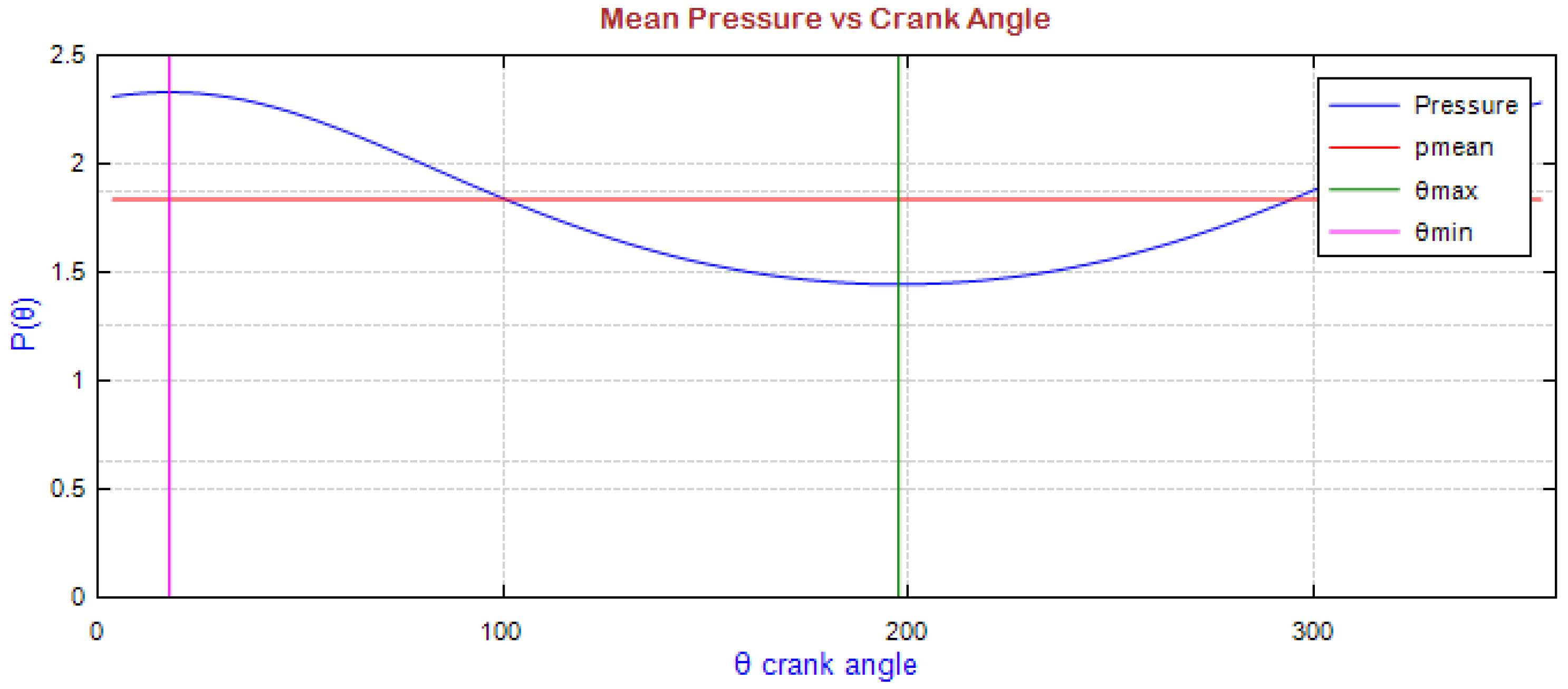
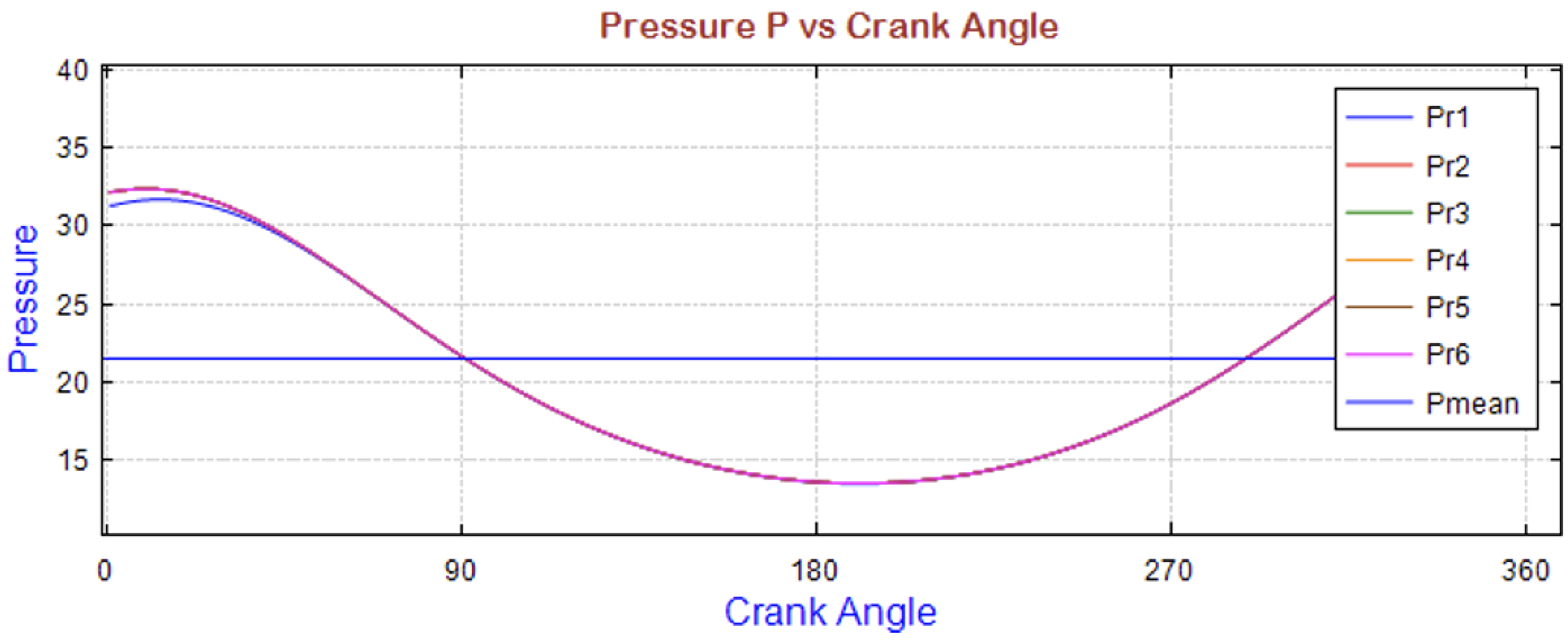
For the application of the isothermal analysis model to the Stirling PPG-102 cryocooler, a computational code was developed. Figure 4 presents the variation in the average pressure of the working fluid in Pa as a function of the crank angle θ . A nearly sinusoidal shape of the variation can be observed, which resulted from both the operation of the kinematic mechanism and the thermodynamic changes that occurred.
The compression process occurred in the first quadrant (0 to 126 degrees). Some part of the compression seemed to take place in the expansion space, but the majority of the working fluid was compressed in the compression space. The displacement process occurred in the second quadrant (126 to 180 degrees) with a constant total volume. The expansion process took place in the third quadrant (180 to 306 degrees), was also non-ideal, and some part of it seemed to occur in the compression space. Finally, the second displacement process occurred in the fourth quadrant (306 to 360 degrees) and appeared to remain incomplete, as some of the working gas remained in the expansion space.
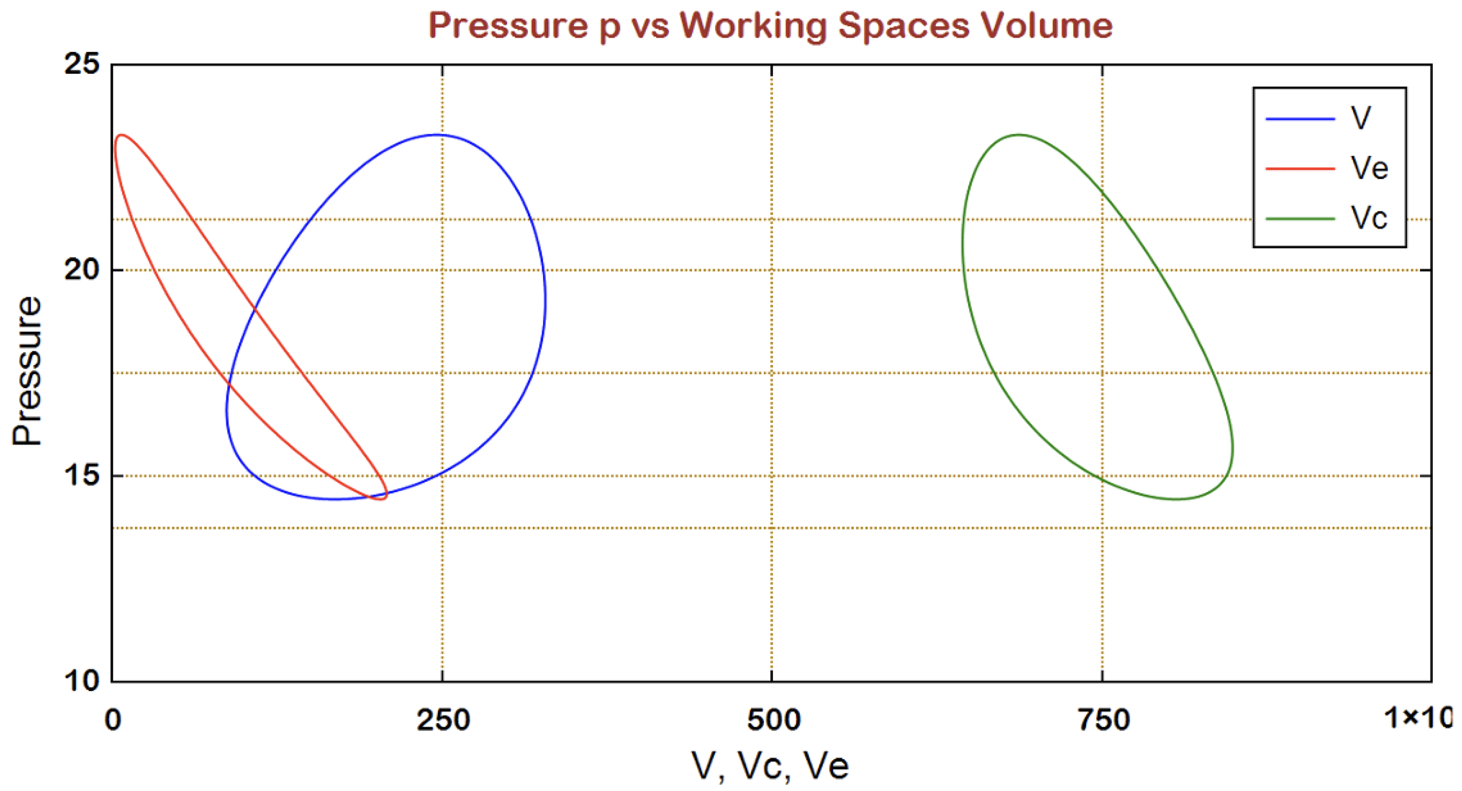
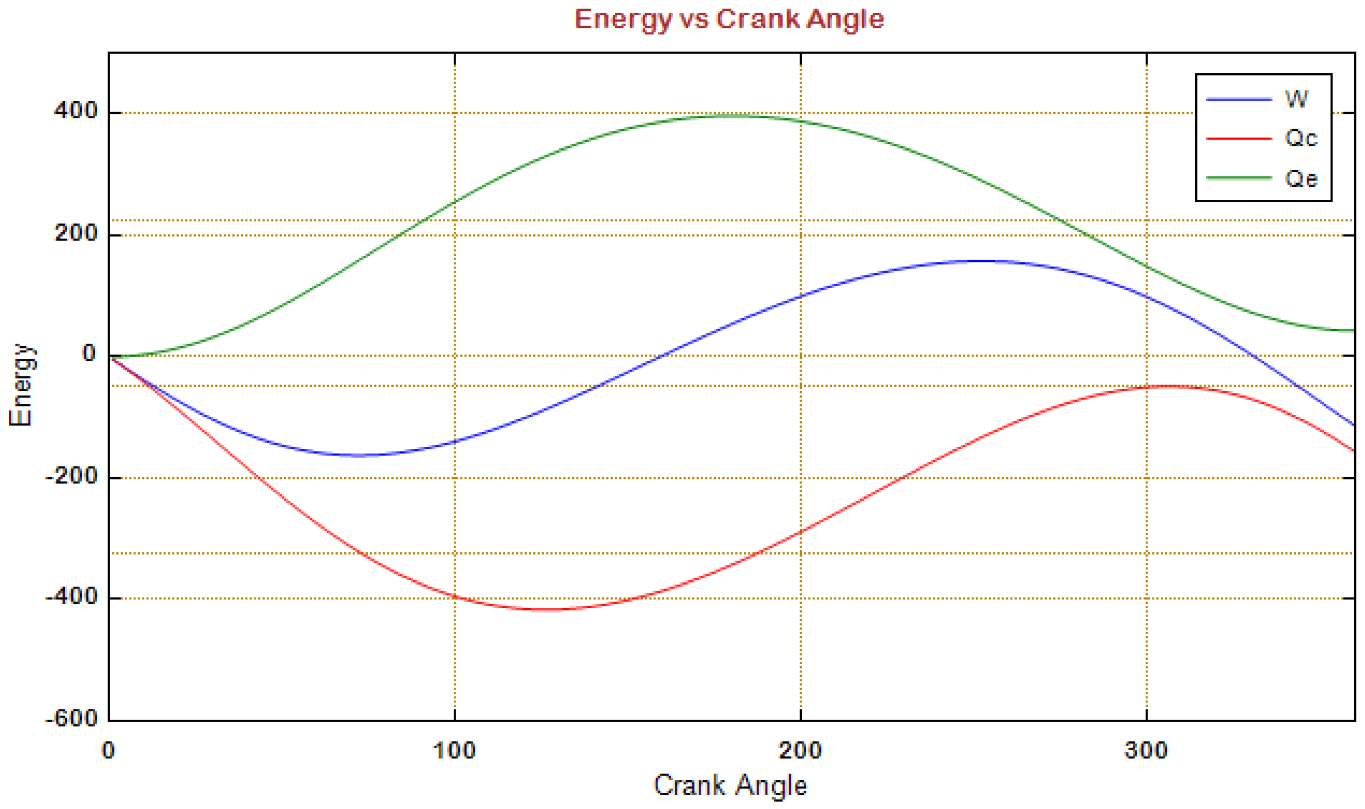
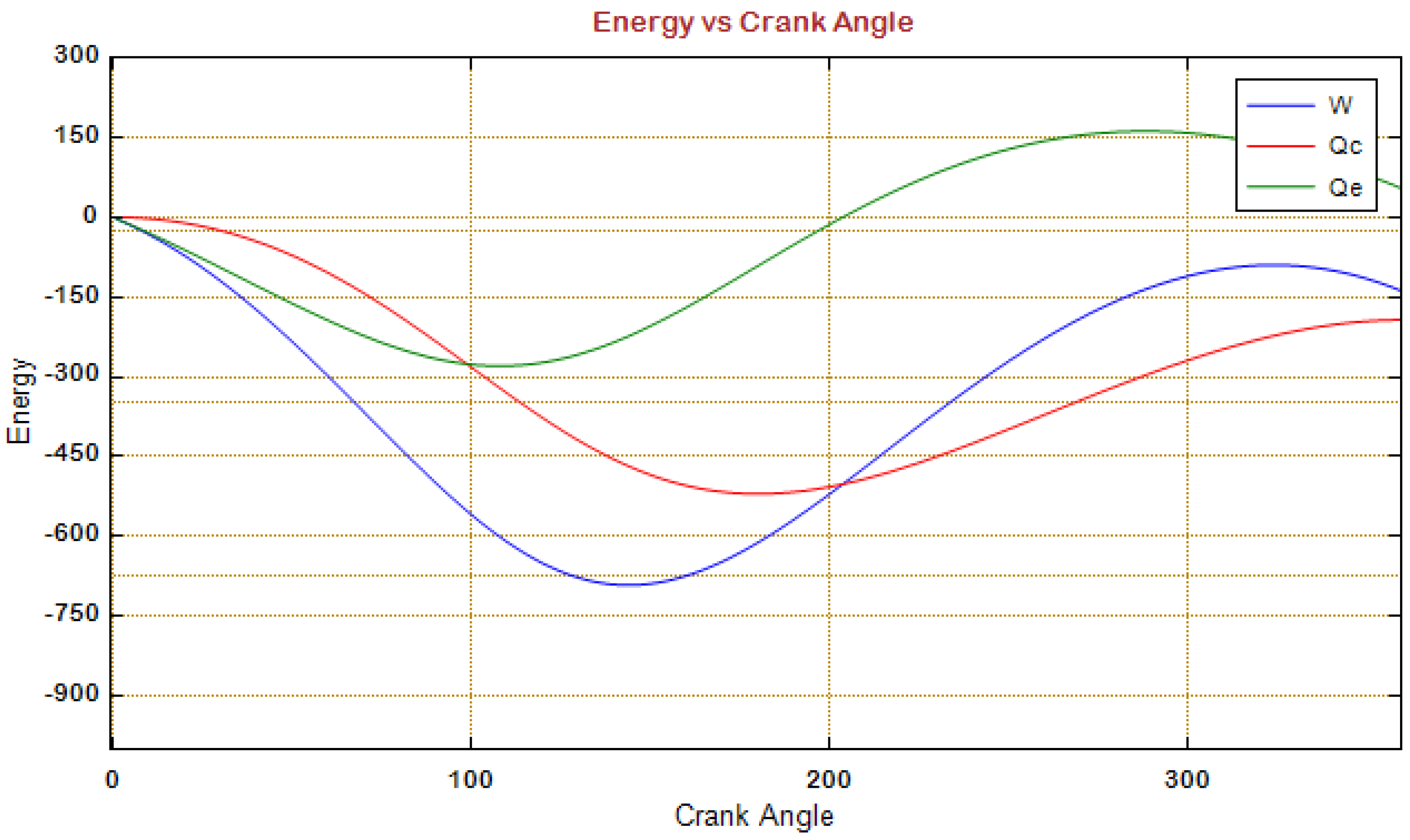
In Figure 5, the P-V diagrams are presented, showing how they were formed in the compression and expansion spaces. The area enclosed by the curves represents the refrigeration work produced in the expansion space, the work consumed in the compression space, and the total required work. The pressure to volume of the entire apparatus is represented by the blue oval, with the green and red ovals representing the compression and expansion volumes, respectively. Since the apparatus is a cryocooler, the work of the expander is equivalent to the cooling power of the cooler in this isothermal model. Similarly, Figure 6 illustrates the accumulated energies per crank angle in joules. The significant fluctuation of energy flows can be observed, as well as the final amount obtained through the completion of the cycle, namely at a crank angle of 360 degrees. It can be seen that the heat of the cooler is positive and the heat of the expander is negative, as expected in a cryocooler with the expander drawing heat from the cold box and providing the cooling power of the apparatus.

4.2. Schmidt Analysis Results

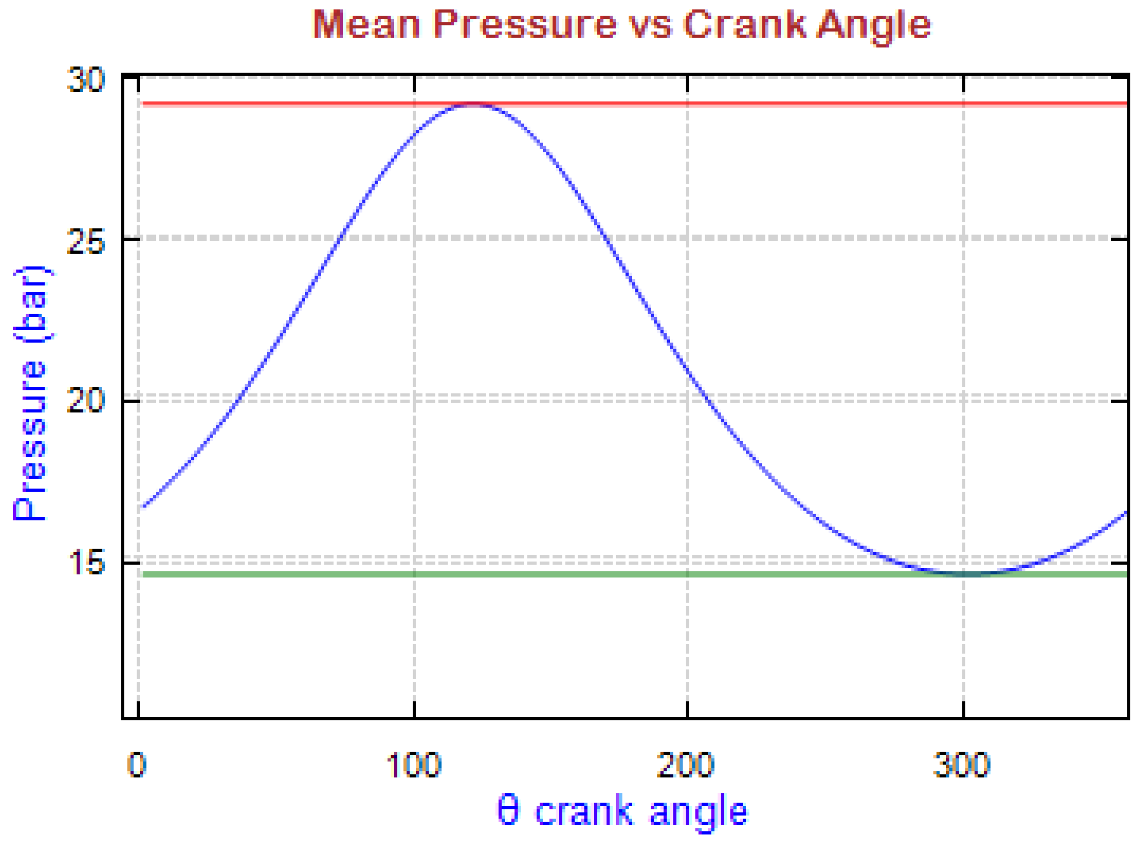
Using the Schmidt analysis, a corresponding computational code was developed, incorporating the geometric characteristics of the machine, the thermophysical properties of the materials, and the working fluid, as well as the operating conditions. Figure 7 illustrates the variation in the average pressure of the working fluid.
In the following figure (Figure 8), a diagram of the accumulated energies as a function of the crank angle is presented, as obtained from the Schmidt analysis. Differentiation can be observed regarding the timing at which the maximum and minimum values occurred, but this is solely due to the arbitrary selection of the initial time moment.
In Table 3, the energy results obtained from the Schmidt analysis are presented, whereas Table 4 presents a comparison of these results and the corresponding results from the isothermal analysis.

4.3. Adiabatic Analysis Results

As mentioned above, the ideal adiabatic model is not a problem of initial conditions but a problem of boundary conditions. We do not know the initial values of the temperatures in the compression spaces, T c , and expansion spaces, T e . The only help we have in selecting the correct initial values is the requirement that these values should be equal to their respective values at the beginning of the cycle. However, due to the cyclic nature of the problem, it can be considered as an initial condition problem. We define some initial conditions, and after a small number of cycle iterations, the conditions and variables should stabilize. Additionally, at the end of each cycle, they should return to their respective values at the beginning of the cycle. Our experience has shown that the most sensitive variable in such problems is the heat exchanged with the regenerator, Q r , which should be zero at the end of each cycle since we are dealing with an adiabatic model. As mentioned before, the temperatures in the compression and expansion spaces are initially set to T k and T h , respectively. The system of equations is solved as many times as needed to stabilize the operating conditions, typically requiring 5 to 10 cycles. Once the initial conditions of the variables are defined, an iterative process (loop) begins with up to 10 iterations, each representing one cycle of operation. The configuration and operating conditions of the PPG-102 cryocooler were described in the isothermal analysis. To analyze the operation of the machine, we need the equations for the volume variations, V c and V e , and their derivatives, D V c and D V e . The initial values of the temperatures in the working compression and expansion spaces are T c = T k and T e = T h , respectively. The initial conditions are set the same as in the isothermal analysis to facilitate the direct comparison of the obtained results. The response of the adiabatic model in the cyclic approximation is sufficient, as the values of the variables, as well as their derivatives with the crank angle, are seen to be equivalent in angles of 0 and 360 after a small number of cycles. Within a time equivalent to four cycles of machine operation, substantial convergence, and stabilization of the operating conditions are observed.
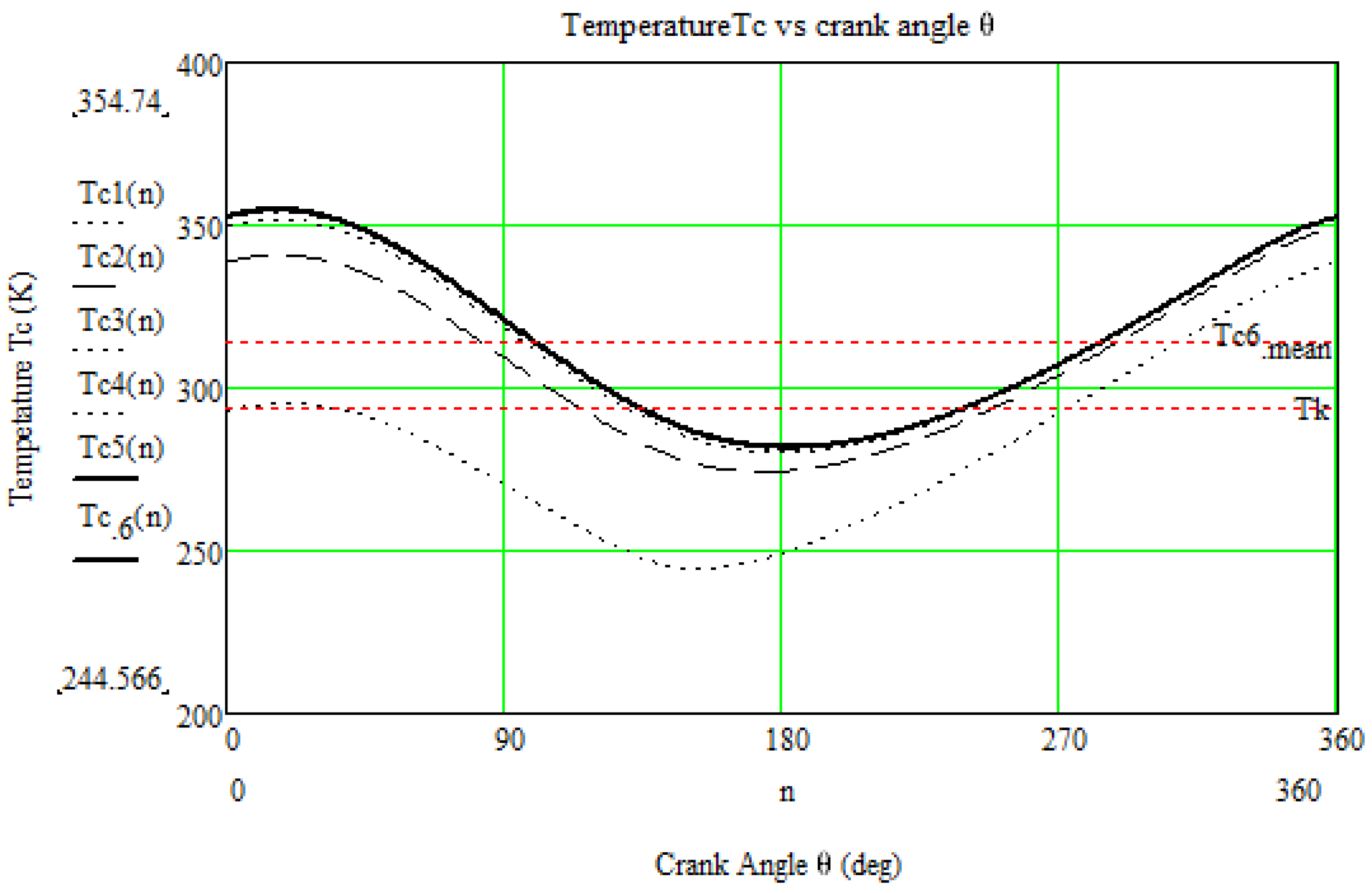
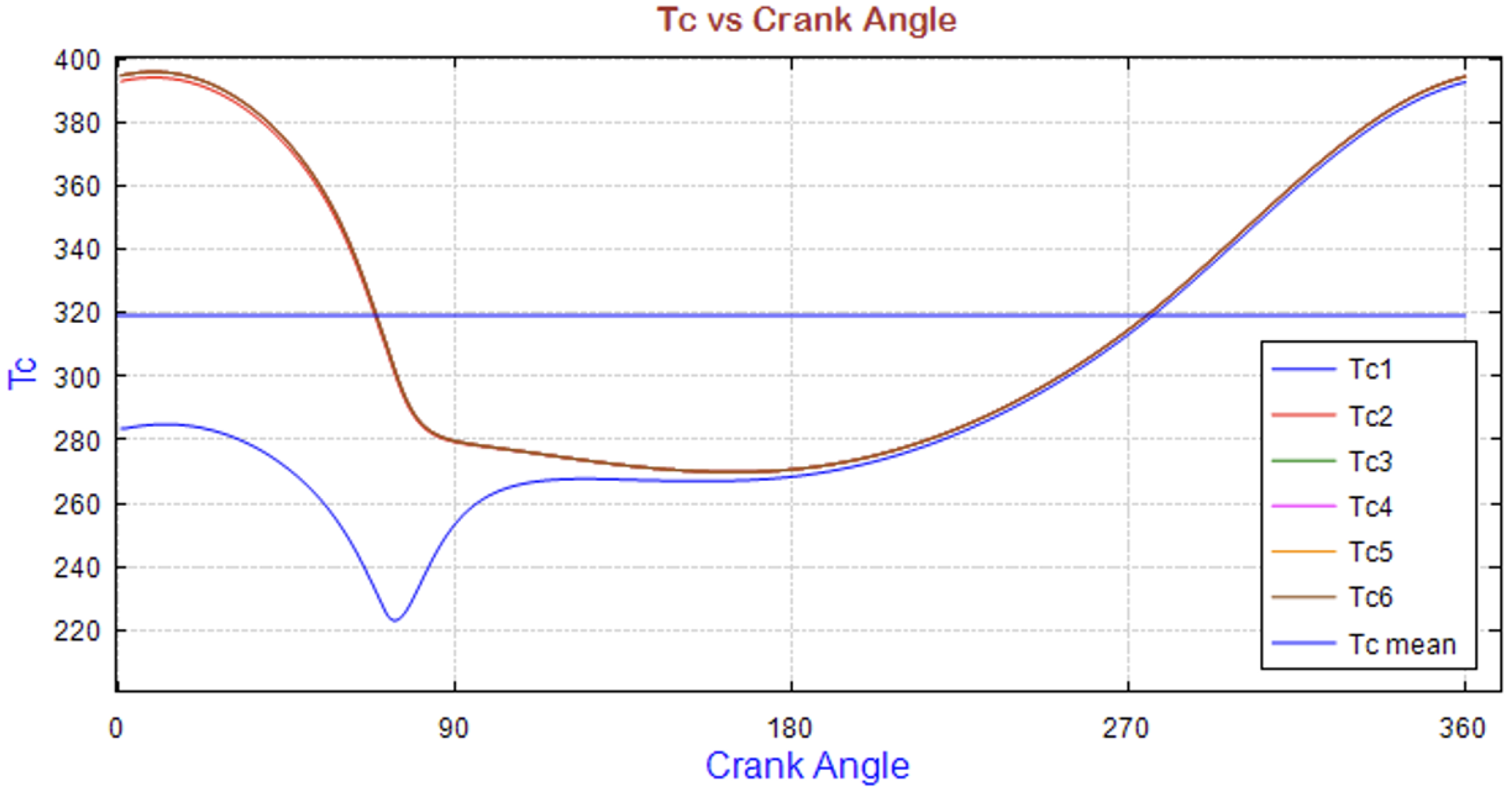
The convergence of the cycle is further showcased in the graphs in Figure 9. Figure 9 illustrates the convergence of the temperature fluctuations during each of the cycles, showing that after a small number of cycles, a near-complete convergence is reached.
After the completion of the second cycle of machine operation, all thermodynamic characteristics are stabilized (Figure 10), which provides further validation of the convergence of the system.
In the figures below, the variations in different parameters as a function of the crank angle θ are presented. In the diagram of the temperature as a function of the crank angle, the large range of the gas temperature fluctuation in the compression space can be observed, which ranged between 220 K and 400 K, with the average temperature significantly higher than the temperature of the heat exchanger, which was 180 K. Similarly, the average temperature of the working gas in the expansion space was lower than the temperature in the cooler. A significant observation is the change in the final coefficient of performance (COP) from 35.56% to 27.27%. The diagram of the energy as a function of the crank angle θ shows the dependence of the transferred heat and required work in the machine’s operating cycle. The power expected from the analysis of the adiabatic model was approximately 1.344 kW. However, the wide range of the temperature fluctuation in the adiabatic working spaces resulted in an increased range of the pressure fluctuation, which led to higher power generation. Both the diagram of the crank angle as a function of θ and the diagram of the heat flow rate as a function of the crank angle show a remarkable relationship between the heat flow rate in the regenerator and the power generated by the machine. This leads us to the conclusion that the performance of the machine is directly connected to the efficiency of the regenerator and its ability to absorb and transfer high heat flows. In Figure 11 and Figure 12 it can be seen that in the adiabatic model, a greater divergence of the temperatures can be seen to occur, which is consistent with previous results such as [16,17].
In Figure 11 and Figure 12, it is evident that the temperatures of the working medium stabilized very quickly, albeit on a theoretical level.
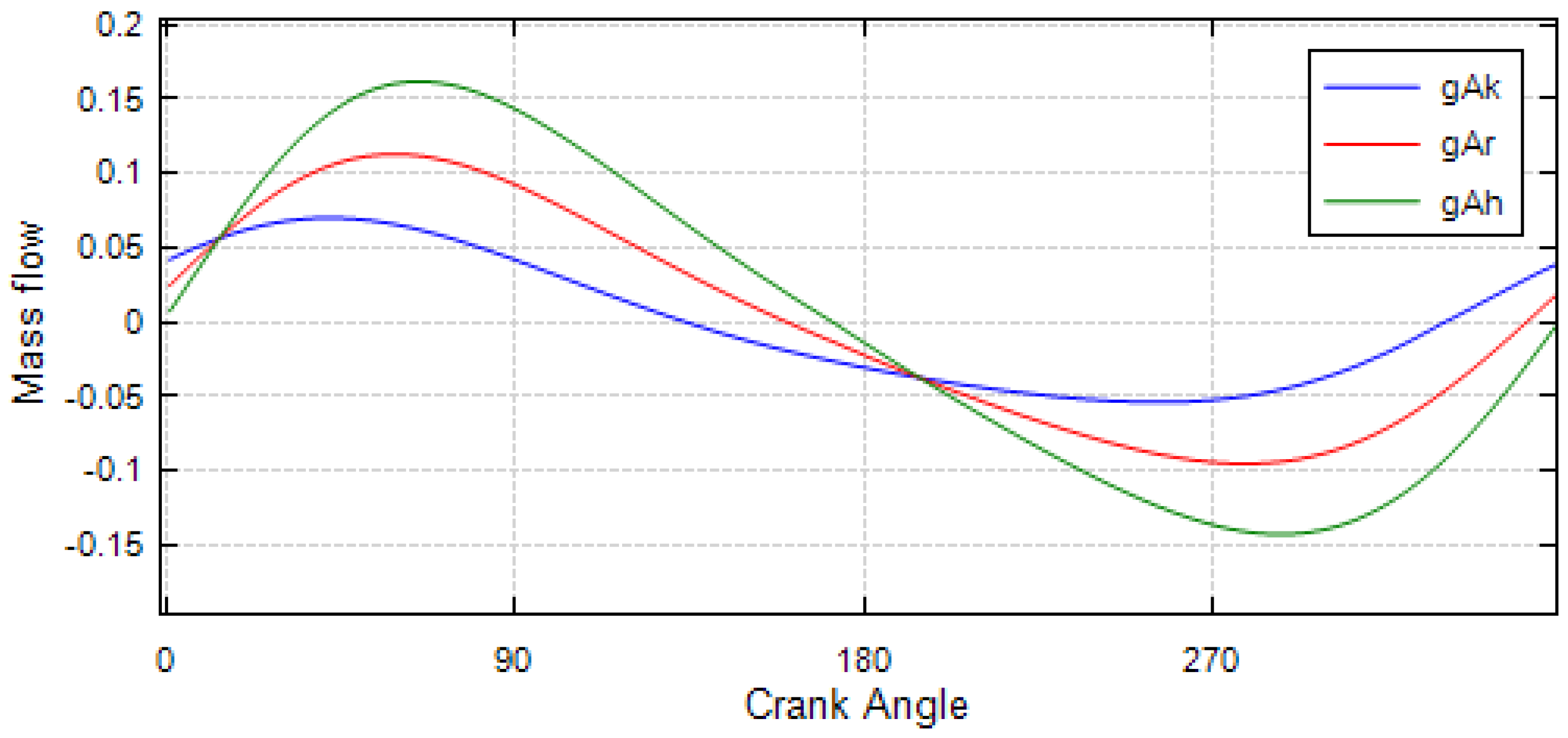
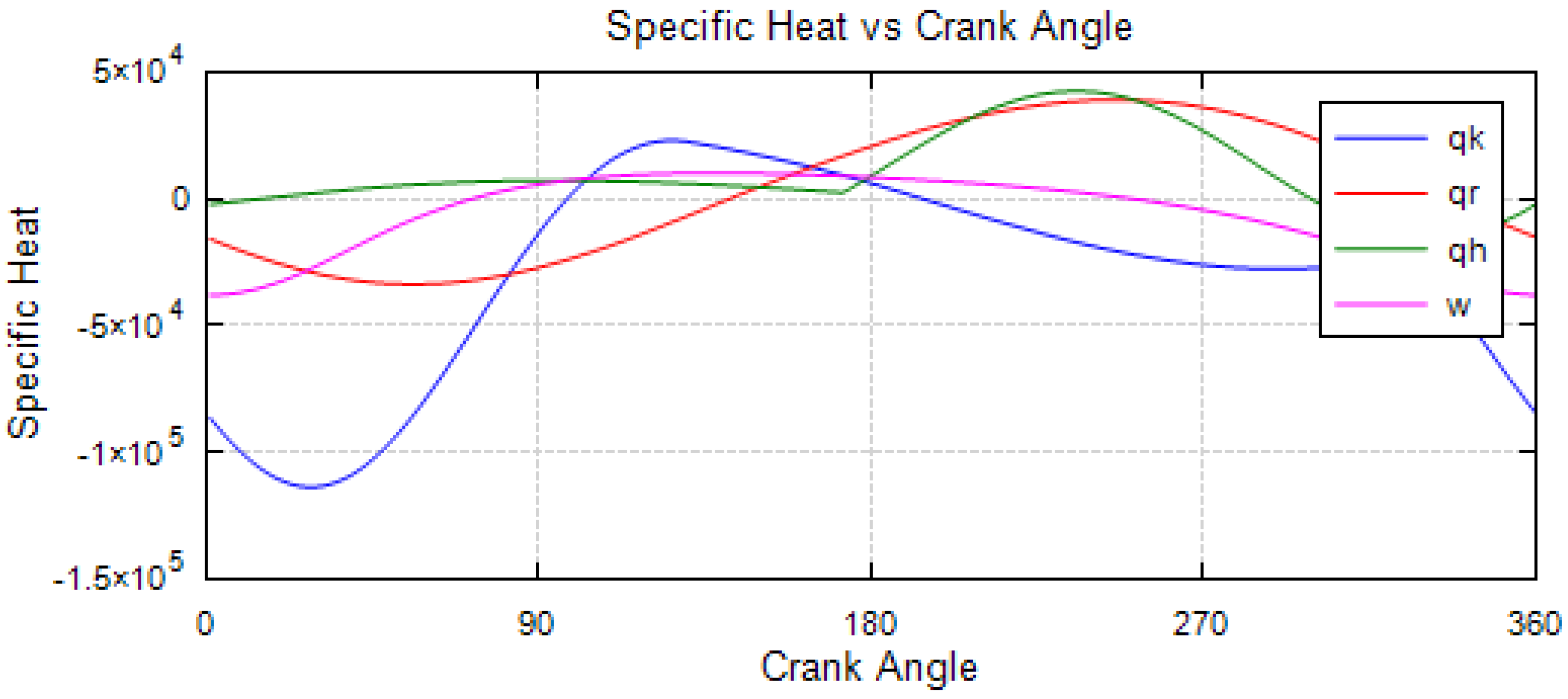
In Figure 13, the specific heat values at the cooler (qk), regenerator (qr), and heater (qh) are presented. Simultaneously, the variations between the specific works (Figure 14) are also shown as a function of the crank angle. The specific results for the adiabatic analysis can be seen in Table 5.
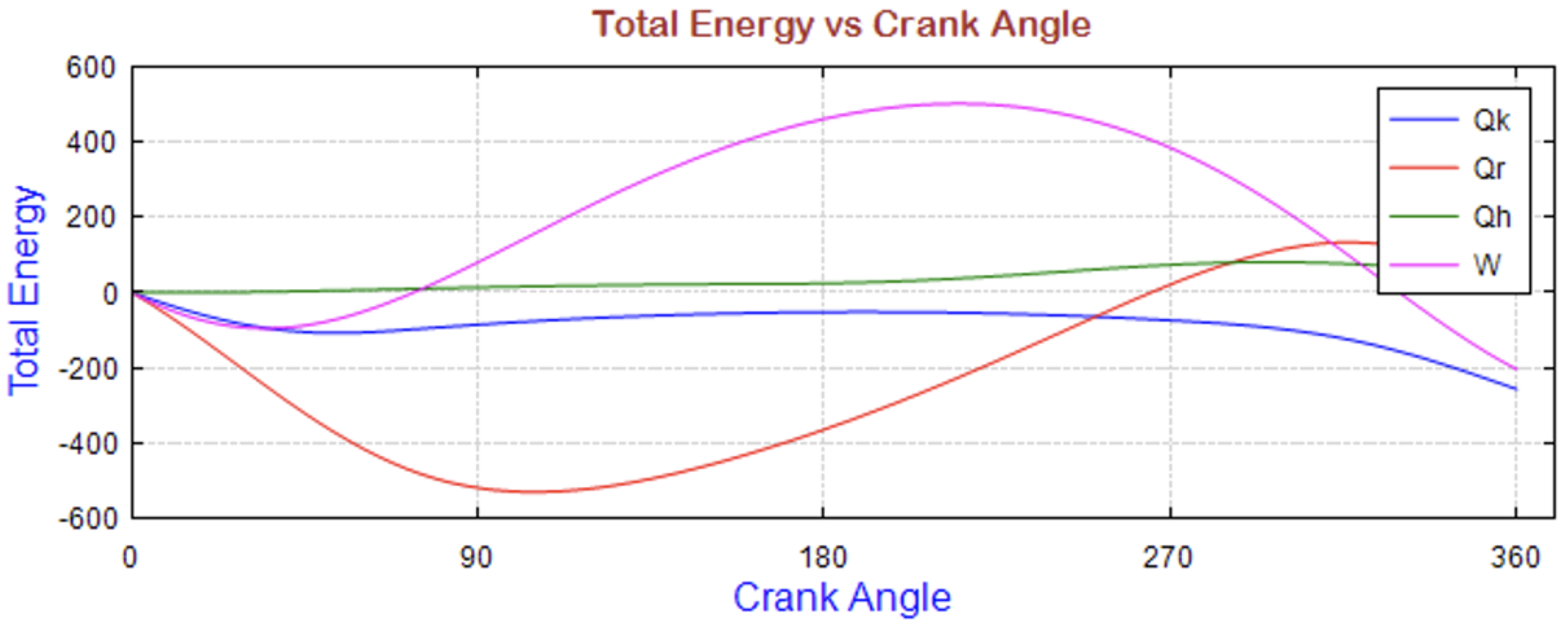
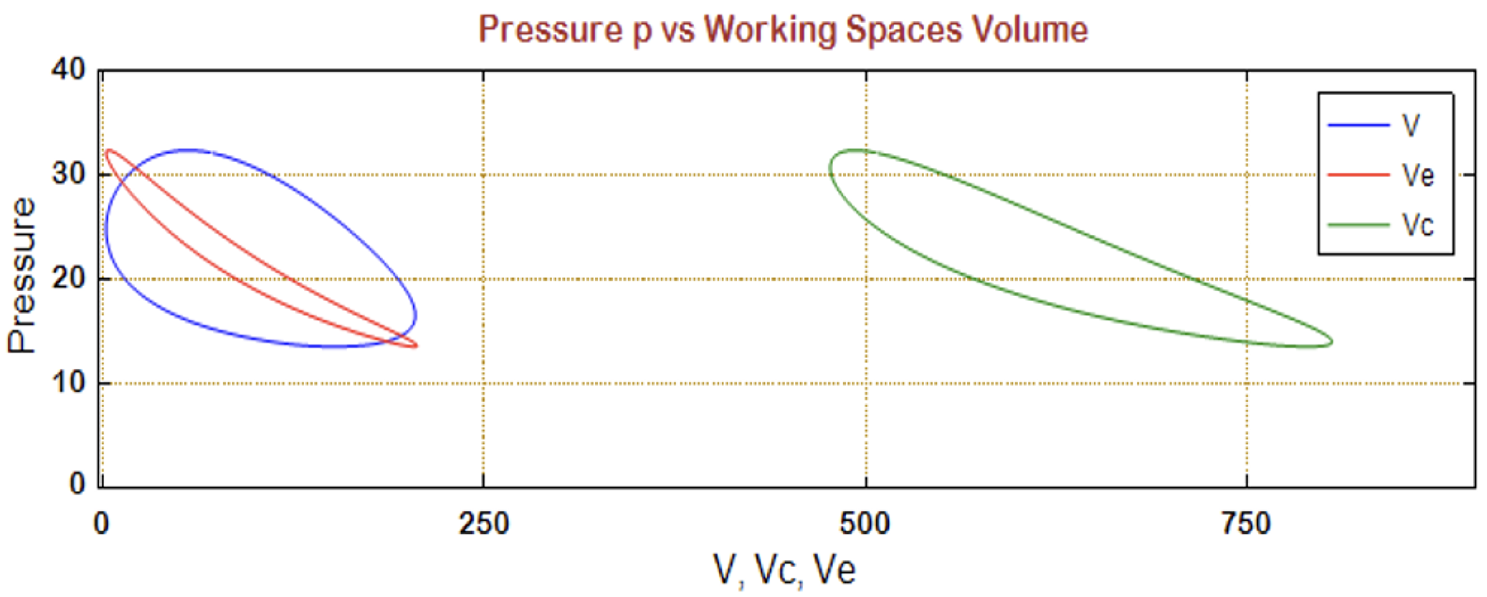
The accumulated energies as a function of the crank angle are presented in Figure 15, whereas Figure 16 shows the P-V diagrams.

4.4. Comparison of Computational Results of Thermodynamic Analysis

Table 6 presents the results obtained from the three models developed for this specific study (isothermal, Schmidt, adiabatic analysis), along with their respective theoretical counterparts according to Walker [7], Altrey et al. [8], and Ruijie et al. [9].

5. Thermal Behavior Simulation of the PPG-102 Thermal Performance in Solidworks Environment

The components involved in the thermal behavior simulation of the PPG-102 in the Solidworks environment were as follows:
  • Power piston and cylinder;
  • Displacer and crankshaft with a phase angle of 90 degrees;
  • Regenerator;
  • Piston housings (base and cylinder);
  • External engine casing;
  • Cooler;
  • Power delivery system;
  • Engine supports.
The design sequence of the individual parts of the engine was carried out from the internal section toward the outer section to avoid any issues during the final digital assembly of the engine. Simultaneously, we ensured its smooth operation under real conditions by including the design of appropriate supports. The schematics of the parts and the assemblies are provided in the Appendix A.
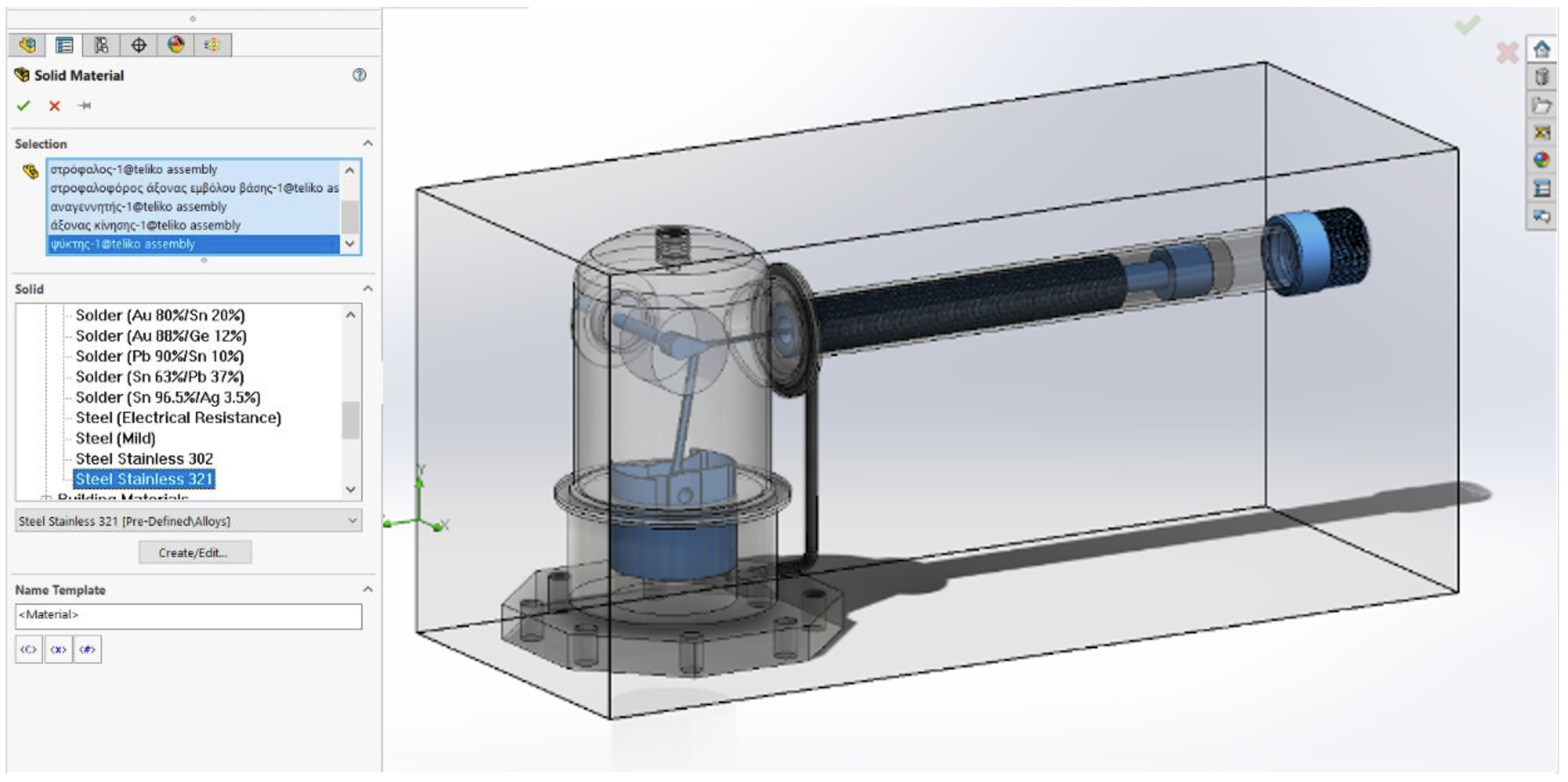
After introducing the initial and boundary conditions into the model, the materials used to build the various parts of the engine were specified (Figure 17).
Upon completing the necessary adjustments regarding the boundary conditions, the required simulation time was determined. At this point, it should be noted that we aimed for a balance between optimal performance and the shortest possible simulation time. Focusing on optimal performance alone can lead to significantly longer simulation times and require correspondingly high computational power, whereas a short simulation time can yield less accurate results. To simulate the apparatus given the designed geometry, all the engine parts were designed in 3D and then combined into a single arrangement. Then, utilizing the “wizard” tool in Solidworks, a flow simulation project was created. The flow characteristics, being the rpm speed, time-dependent heat transfer parameters for the chosen materials (as found in the literature [18]), and the working medium, were chosen. Helium, as the optimal working medium for the temperature range of this simulation, was used and modeled as an ideal gas according to the Solidworks libraries. According to the cryogenic behavior of helium, at these temperatures, the assumption of an ideal gas provides an excellent representation [19]. Aluminum was chosen for the parts of the machine, and given the extensive libraries in Solidworks in Al., the included models were used. The roughness of the walls was implemented in the model, and the initial conditions based on the environment were chosen. Overall, by setting the system as described, the simulation proceeded, without any need to specify either an isothermal or adiabatic model, giving us the best possible representation of the system based on its properties. Through this simulation, the full thermodynamic analysis of such an apparatus at cryogenic temperatures, without forcing any model upon the simulation, was achieved, and the results are presented below.
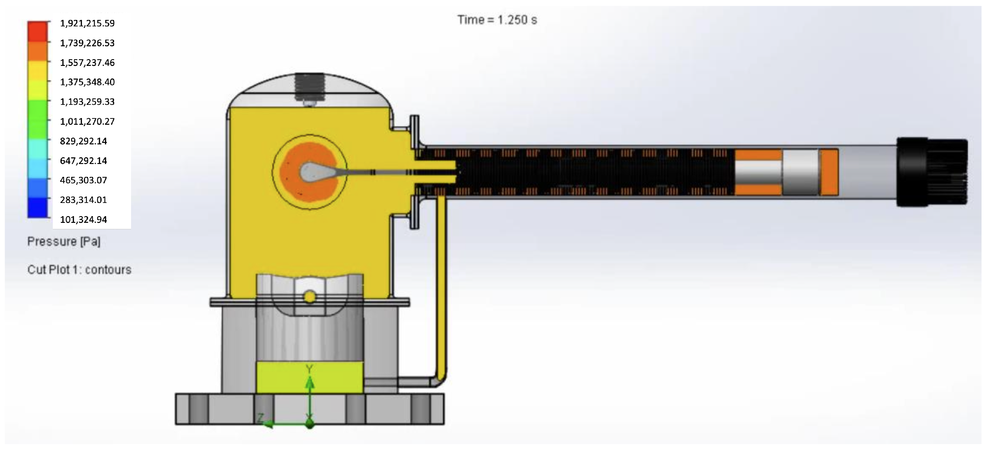
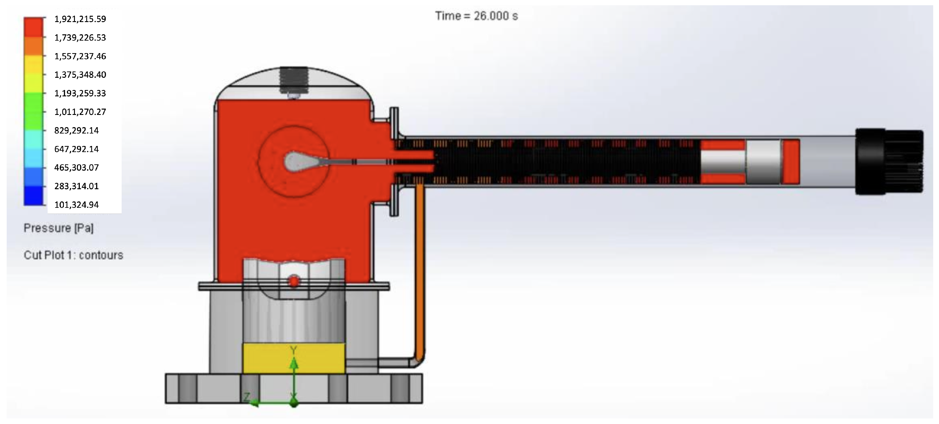
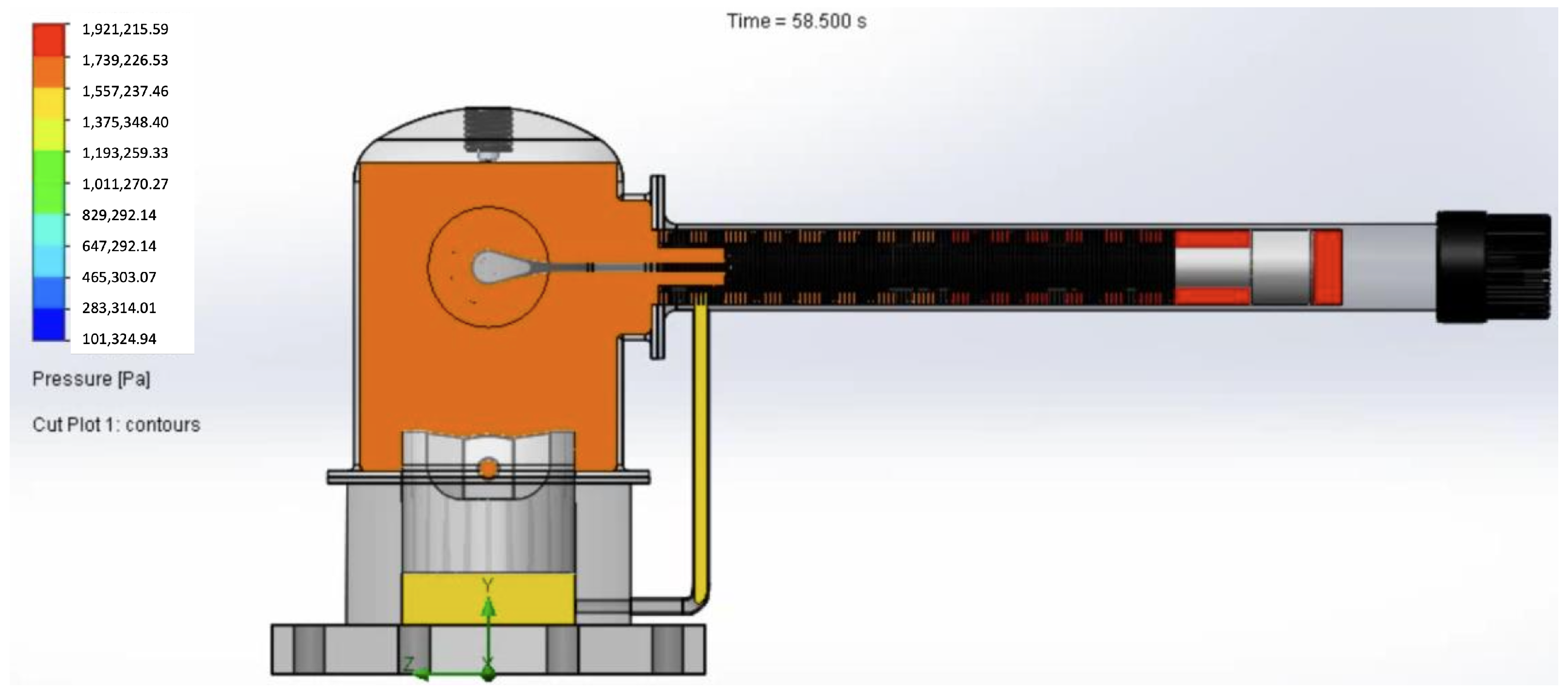
In Figure 18, Figure 19 and Figure 20, the pressure fluctuations are presented at time points of 1.25, 26, and 58.5 s after reaching the steady state in the simulation.
The following diagram in Figure 21 presents the minimum, maximum, and average pressure values in the compression and expansion chambers.
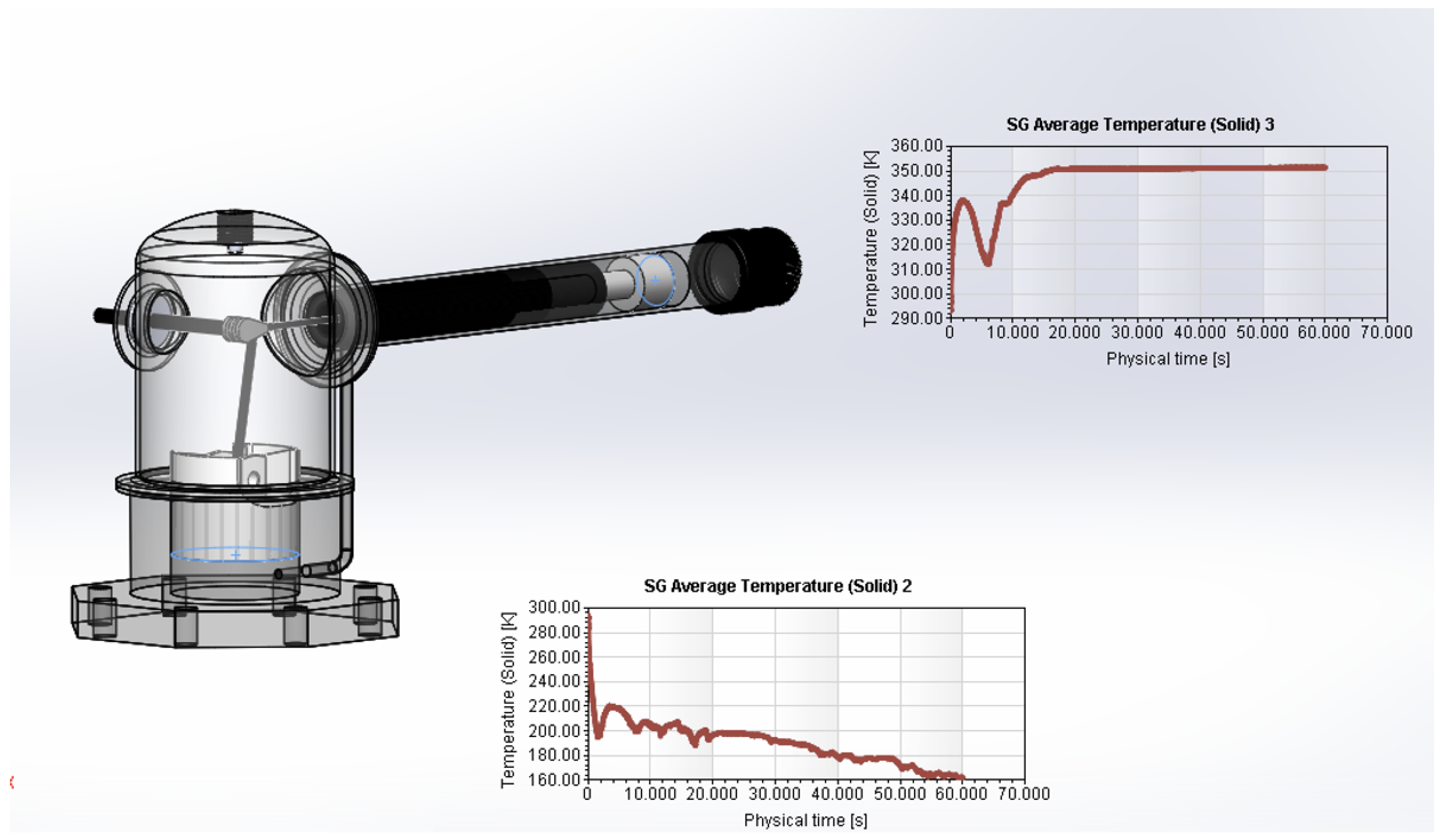
In Figure 22, the temperature variation of the working fluid is presented for both the cooler and the freezer, from the start of the simulation until thermal equilibrium is reached.
With the simulation, it was possible to extract pressure and temperature results at each level along the internal space of the engine and identify points where our model experienced a higher load. Additionally, as seen in Figure 18, Figure 19 and Figure 20, it was possible to calculate the pressures exerted by the fluid during its motion, even on the solid parts of the engine. This information can be utilized to assess stresses and the overall lifespan of the model under specific operating conditions. However, one limitation of the simulation is that it did not allow for the simultaneous prediction of both the model’s motion and the fluid flow. Therefore, the analysis was conducted over a one-minute time interval instead of infinite operating conditions. During the simulation, the temperature at the exhaust end stabilized at 160 K, whereas in the compressor, it stabilized at 350 K. Similarly, the average pressure throughout the entire engine interior was approximately 18 MPa. This behavior appears to be similar to the results obtained from the adiabatic analysis in the code.

6. Conclusions

In this study, three different thermodynamic analysis models for Stirling engines were developed and applied: the isothermal model, the ideal Schmidt model, and the ideal adiabatic model. These models were implemented on the well-known PPG-102 cryogenic engine. Subsequently, a comparison was carried out between the theoretical results obtained from the three developed analysis models and the corresponding theoretical results presented by Walker [7], Atrey et al. [8], and Ruijie et al. [9]. The comparison showed significant convergence of the results, and any deviations were primarily attributed to the assumptions of each model. Finally, the engine was designed in the Solidworks environment, and a simulation was performed under the same operating conditions as those of the computational models developed. The simulation results closely approximated those of the adiabatic analysis, which was expected. The utilization of multiple analysis models, along with the incorporation of a comprehensive simulation approach, can lead to a more comprehensive understanding of the thermodynamic behavior and performance of the PPG-102 cryogenic engine. These findings enhance the existing knowledge and provide valuable insights into the design and optimization of Stirling engines for cryogenic applications. As demonstrated in this study, the augmentation and utilization of traditional models developed for thermal Stirling engines led to an in-depth understanding of both thermodynamic and fluid mechanic behaviors when applied to a cryogenic engine. In addition, the relative convergence of the three models supported the provided results, given that the systems operated at relatively low speeds. At lower speeds, it is known that the adiabatic model for Stirling coolers converges with the isothermal model [17], something that can be directly observed in the provided results. Moreover, as the ideal adiabatic model calculates the pressure drop due to the flow of the working medium, it was expected that the differentiation between the results would be mitigated. The isothermal and Schmidt models are similar in terms of the principles they use for the thermodynamic analysis of the apparatus. Therefore, it is expected that they would yield converging results, providing a form of cross-validation for the model when their results are compared. As far as the ranges of the models are concerned, the presented models were compared using the provided thermodynamic descriptions, taking into account the different levels of analysis they offered. As such, given the results of this work, the authors suggest that if a Stirling cooler with a higher rpm is used, the adiabatic model is the better choice; otherwise, for lower working speeds, the isothermal or Schmidt models are sufficient. Further research endeavors could explore the refinement of the analysis models by incorporating additional factors, such as fluid dynamics and heat transfer characteristics, as well as conducting experimental validation to enhance the accuracy and reliability of the proposed models. Such advancements will contribute to the advancement of Stirling engine technology and foster its widespread implementation in various cryogenic applications.

Author Contributions

Methodology, G.A. and I.K.; Software, G.A. and S.B.; Validation, G.A.; Formal analysis, G.A.; Investigation, G.A. and G.-R.D.; Resources, G.A. and G.-R.D.; Data curation, G.A. and G.-R.D.; Writing—original draft, G.A.; Writing—review & editing, G.-R.D. and S.B.; Supervision, I.K.; Project administration, I.K. All authors have read and agreed to the published version of the manuscript.

Funding

This research received no external funding.

Data Availability Statement

The data used in this research are presented in this work.

Conflicts of Interest

The authors have no conflict of interest to declare.

Nomenclature

g A r mass flow rate ( k g / s )
Tworking gas temperature (K)
Qheat rate (W)
Wwork ( J / c y c l e )
W e consumed work by the displacer piston per cycle ( J / c y c l e )
Ppower output (W)
Mworking gas total mass ( k g )

Appendix A

Table A1. Basic specifications of the cryocooler.
General
Machine Type (Configuration)B
Number of Cylinders1
Piston Drive MechanismPhilips-crankshaft
Working FluidHelium
Mass of He M = 4.808 g
Mean Pressure p m e a n = 22 bar
Frequency f = 24.167 Hz
Mean Phase Difference between Pistons 72
Active Exhaust Space Temperature T e = 77.1250 K
Cold Metal Temperature T h = 80 K
Exhaust Temperature Difference Δ T e = 2.8750 K
Active Compression Space Temperature T c = 352.5 K
Cooling Water Temperature T k = 293.86 K
Compression Temperature Difference Δ T c = 58.64 K
Displacement Volume of Compression V c l c = 1.924 cc
Displacement Volume of Exhaust V c l e = 1.924 cc
Swept Volume in Compression V s w c = 202.804 cc
Swept Volume in Exhaust V s w e = 203.968 cc
Maximum “Dead” Volume V m a x l i v = 324.157 cm
Minimum “Dead” Volume V m i n l i v = 82.633 cm
Cooler Volume V k = 42.127 cc
- Regenerator Volume V r = 379.463 cc
- Condenser Volume V h = 12.668 cc
- Cylinder Diameter7.00 cm
- Displacer Clearance Diameter0.500 cm
- Clearance at End of Piston0.050 cm
- Clearance at End of Displacer0.050 cm
- Clearance Gap of Exhaust Cover0.040 cm
- Length of Exhaust Cover10.000 cm
- Clearance Volume of Exhaust Cylinder1.924 cc
- Clearance Volume of Compression Cylinder1.924 cc
- Bugger Factor1.000
- Cold Water Flow Rate1.000 L/s
- Thermal Conductivity of Metal0.010 W/m·K
- Mechanical Efficiency70%
- Thickness of Exhaust Cylinder Wall0.250 cm
- Thickness of Exhaust Cover Wall0.250 cm
- Thickness of Regenerator Protective Cover0.250 cm
- Internal Diameter of Cooler Tubes0.160 cm
- Length of Cooler Tubes10.00 cm
- Length of Heat Transfer10.00 cm
- Number of Cooler Tubes per Cylinder200
- External Diameter of Regenerator12.700 cm
- Internal Diameter of Regenerator7.620 cm
- Length of Regenerator7.620 cm
- Number of Regenerators per Cylinder1
- Diameter of Wire Mesh0.008 cm
- Void Fraction0.400
- Surface Area per Unit Volume179.000 cm 2 /cm 3
- Weave Density (Threads per cm)63.662
- Internal Diameter of Freezer Tubes0.100 cm
- Length of Freezer Tubes7.600 cm
- Length of Heat Transfer7.600 cm
- Number of Freezer Tubes per Cylinder180
- Length of Connecting Displacer15.000 cm
Length of Pulley2.650 cm

3D Schematics

In this section, representative 3D schematics from the Solidworks software are included for the reader to better understand the system and simulation.
The following figures illustrate the 3D designs of the basic parts of the PPG-102 according to the dimensions presented in Table 3.
Figure A1. The power piston of the Stirling PPG-102 cryocooler.
Energies 16 06815 g0a1
Figure A2. The kinematic mechanism of the PPG-102 cryocooler.
Energies 16 06815 g0a2
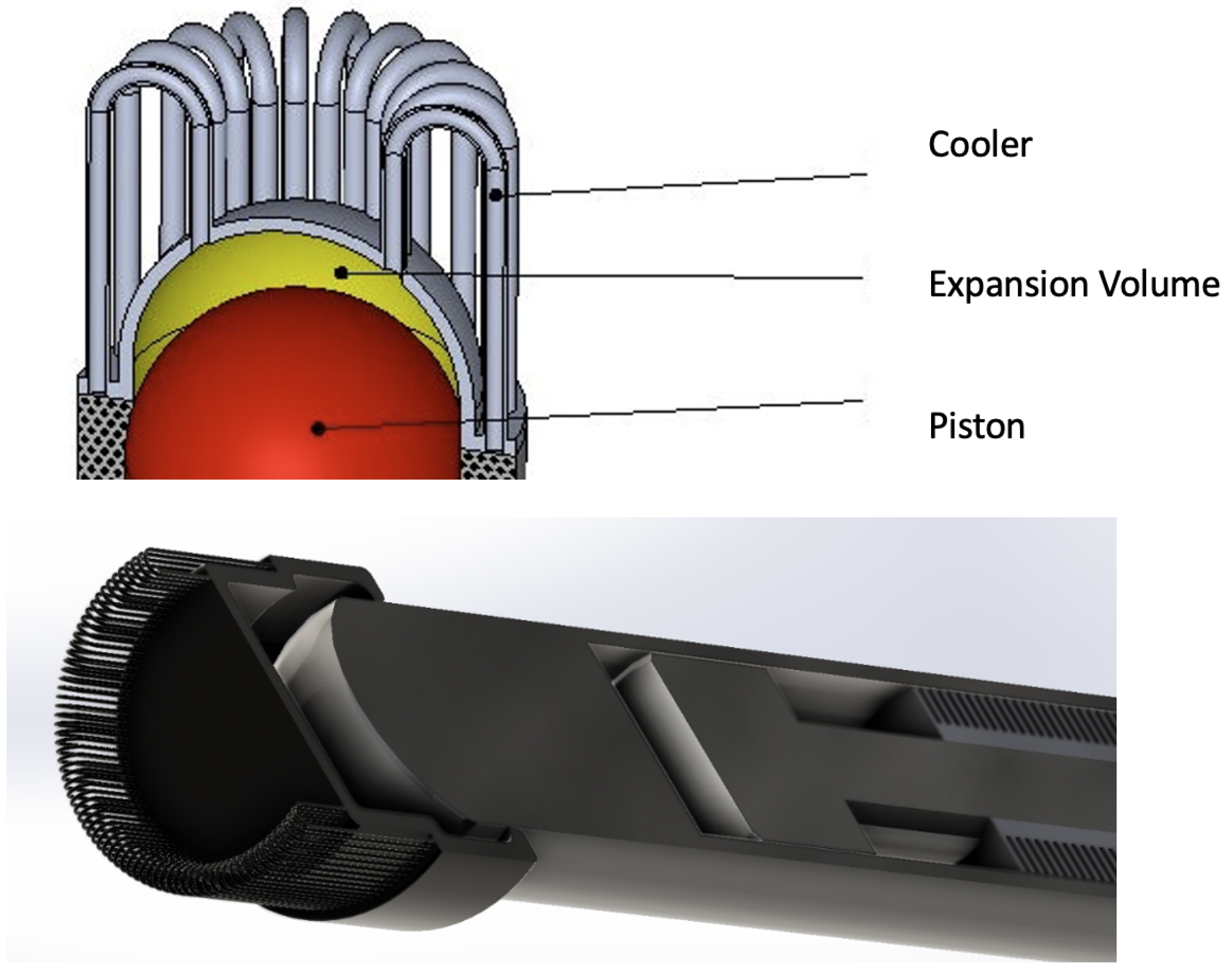
Figure A3 depicts a detailed view of the cooler of the engine, including the compression chamber and the power piston.
Figure A3. Some detail of the heat rejection end of the engine is shown.
Energies 16 06815 g0a3
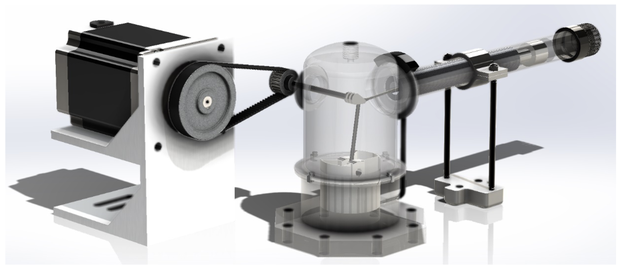
The final three-dimensional model used for the simulation analysis is presented in Figure A4.
Figure A4. The kinematic mechanism of the PPG-102 Stirling engine with the regenerator.
Energies 16 06815 g0a4

References

  1. Walker, G. Cryocoolers; Springer: New York, NY, USA, 1990. [Google Scholar]
  2. Chen, N.C.; Griffin, F.P. Review of Stirling-Engine Mathematical Models; Oak Ridge National Lab. (ORNL): Oak Ridge, TN, USA, 1983. [CrossRef]
  3. Kongtragool, B.; Wongwises, S. A review of solar-powered Stirling engines and low temperature differential Stirling engines. Renew. Sustain. Energy Rev. 2003, 7, 131–154. [Google Scholar] [CrossRef]
  4. Collins, S.C.; Cannaday, R.L. Expansion Machines for Low Temperature Processes; Oxford University Press: London, UK, 1958. [Google Scholar]
  5. Martini, W. Stirling Engine Design Manual; Technical Report; NASA National Technical Information Services, US Department of Commerce: Spring Field, VA, USA, 1978.
  6. Martini, W. A non-proprietary nonsecret program for calculating Stirling cryocoolers. In Proceedings of the Third Cryocooler Conference, Boulder, CO, USA, 17–18 September 1984; NBS Spec. Pub 698. NTIS: Springfield, VA, USA, 1984. [Google Scholar]
  7. Walker, G.; Weiss, M.; Fauvel, R.; Reader, G. Microcomputer simulation of Stirling cryocoolers. Cryogenics 1989, 29, 846–849. [Google Scholar] [CrossRef]
  8. Atrey, M.D.; Bapat, S.; Narayankhedkar, K. Cyclic simulation of Stirling cryocoolers. Cryogenics 1990, 30, 341–347. [Google Scholar] [CrossRef]
  9. Li, R.; Grosu, L. Parameter effect analysis for a Stirling cryocooler. Int. J. Refrig. 2017, 80, 92–105. [Google Scholar] [CrossRef]
  10. Rogdakis, E.D.; Borbilas, N.A. Second Law Analysis of a Stirling Cryocooler with Optimal Design of the Regenerator and Losses. In Proceedings of the IMCE ASME International Mechanical Engineering Congress and Exposition, New York, NY, USA, 11–16 November 2001. [Google Scholar]
  11. Urieli, I.; Berchowitz, D. Stirling Cycle Engine Analysis; Adam Hilger Ltd.: Bristol, UK, 1984. [Google Scholar]
  12. Schmidt, G. The theory of Lehmann’s Calorimetric Machine. Z. Ver. Dtsch. Ing. 1871, 15, 98–112. [Google Scholar]
  13. Domenikos, G.R.; Bitsikas, P.; Rogdakis, E. Thermodynamic Modelling of Superfluid Stirling Cryocoolers. In Proceedings of the ASME International Mechanical Engineering Congress and Exposition, Salt Lake City, UT, USA, 11–14 November 2019; American Society of Mechanical Engineers: New York, NY, USA, 2019; Volume 59438, p. V006T06A069. [Google Scholar]
  14. Rogdakis, E.; Bitsikas, P.; Dogkas, G.; Antonakos, G. Three-dimensional CFD study of a β-type Stirling Engine. Therm. Sci. Eng. Prog. 2019, 11, 302–316. [Google Scholar] [CrossRef]
  15. Bitsikas, P.; Rogdakis, E.; Dogkas, G. CFD study of heat transfer in Stirling engine regenerator. Therm. Sci. Eng. Prog. 2020, 17, 100492. [Google Scholar] [CrossRef]
  16. Domenikos, G.R.; Bitsikas, P.; Rogdakis, E. Computational Analysis of Cryogenic Stirling Refrigerator. In Proceedings of the ASME 2019 International Mechanical Engineering Congress and Exposition, Salt Lake City, UT, USA, 11–14 November 2019; American Society of Mechanical Engineers Digital Collection: Lawrence, KS, USA. [Google Scholar]
  17. Domenikos, G.R.; Rogdakis, E.; Koronaki, I. Computational Analysis, Three-Dimensional Simulation, and Optimization of Superfluid Stirling Cryocooler. J. Energy Resour. Technol. 2023, 145, 111701. [Google Scholar] [CrossRef]
  18. Amundsen, T.; Furuseth, O.; Sovik, R. The lattice thermal conductivity of aluminium at low temperatures (and dilute aluminium-copper alloys). J. Phys. F Met. Phys. 1977, 7, L159. [Google Scholar] [CrossRef]
  19. Domenikos, G.; Rogdakis, E.; Koronaki, I. Continuous equation of state and thermodynamic maps for cryogenic helium 4. In Proceedings of the ASME International Mechanical Engineering Congress and Exposition, Virtual, 1–5 November 2021; American Society of Mechanical Engineers: New York, NY, USA, 2021; Volume 85642, p. V08BT08A009. [Google Scholar]
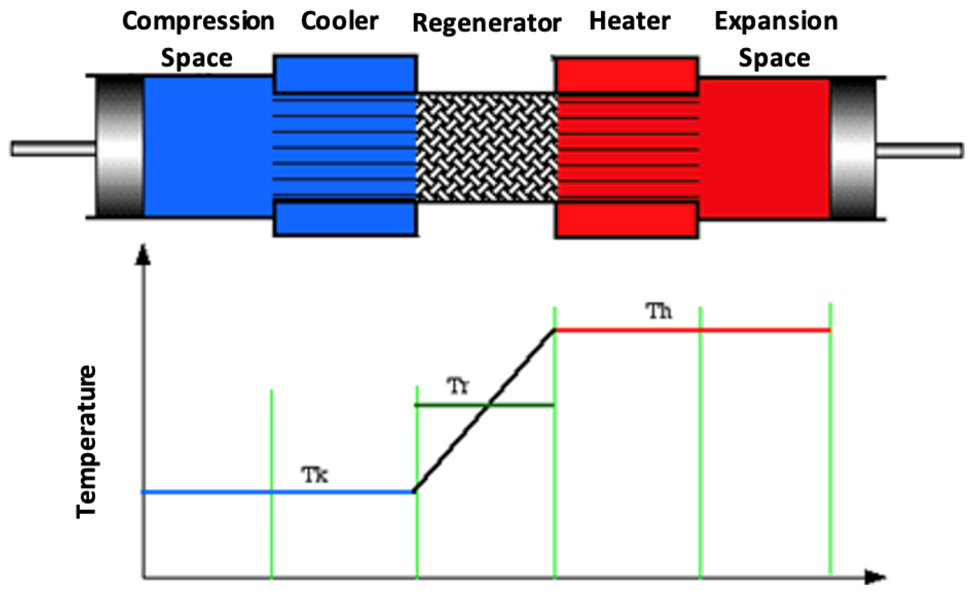
Figure 1. The isothermal model for thermal Stirling engines. The blue color refers to the low temperature and the red color to the high temperature of the cycle.
Energies 16 06815 g001
Figure 2. Typical cell enclosure of the working medium.
Energies 16 06815 g002
Figure 3. The ideal adiabatic model for thermal Stirling engines.
Energies 16 06815 g003
Figure 4. Isothermal analysis: mean pressure (Pa) vs. crank angle of working fluid (helium).
Energies 16 06815 g004
Figure 5. Pressure (bar)–volume (cm 3 ) diagrams for the expansion and compression spaces in an isothermal analysis.
Energies 16 06815 g005
Figure 6. Energy flows (J) vs. crank angle in an isothermal analysis.
Energies 16 06815 g006
Figure 7. Mean pressure vs. crank angle. The red line signified the maximum pressure and the green line the minimum pressure, while the blue line is the mean pressure.
Energies 16 06815 g007
Figure 8. Schmidt analysis energy flows (J) vs. crank angle.
Energies 16 06815 g008
Figure 9. Working fluid pressure vs. crank angle for the first 6 cycles of the simulation. It is seen that as the cycles progress there is a greater leading to full convergence of the Temperature values and fluctuations.
Energies 16 06815 g009
Figure 10. Working fluid pressure vs. crank angle for the first 6 cycles of the simulation. It is seen that from the second cycle the temperature converges with the equivalent lines overlapping.
Energies 16 06815 g010
Figure 11. Working fluid temperature of the hot end of the engine (freezer) vs. crank angle. As per the previous graph, it is seen that from the second cycle the temperature converges with the equivalent lines overlapping.
Energies 16 06815 g011
Figure 12. Working fluid temperature of the cold end of the engine (cooler) vs. crank angle. It is seen again that from the second cycle the temperature converges with the equivalent lines overlapping.
Energies 16 06815 g012
Figure 13. Working fluid mass flow in the engine’s working spaces vs. crank angle.
Energies 16 06815 g013
Figure 14. Accumulated specific heat vs. crank angle.
Energies 16 06815 g014
Figure 15. Accumulated energy vs. crank angle.
Energies 16 06815 g015
Figure 16. Pressure–volume diagrams in the adiabatic analysis.
Energies 16 06815 g016
Figure 17. Specification for the materials used for the construction of the various parts of the Stirling PPG-102 cryocooler.
Energies 16 06815 g017
Figure 18. The pressure fluctuation diagram at the time point of 1.25 s.
Energies 16 06815 g018
Figure 19. The pressure fluctuation diagram at the time point of 26 s.
Energies 16 06815 g019
Figure 20. The pressure fluctuation diagram at the time point of 58.5 s.
Energies 16 06815 g020
Figure 21. The extreme values of the working fluid pressure in various parts of the engine.
Energies 16 06815 g021
Figure 22. Temperature fluctuation toward the steady state.
Energies 16 06815 g022
Table 1. Fundamental Equations used.
p = M R ( V c T k + V k T k + V r l n ( T h T k ) T h T k + V h T h + V e T h ) 1 Pressure
Q e = W e = p d V e d θ d θ Transferred heat to the expansion space
Q c = W c = p d V c d θ d θ Transferred heat to the compression space
W = W e + W c Required work
C O P = Q e W Coefficient of performance (COP)
Table 2. Key results from adiabatic thermodynamic.
Required work W = 114.115 J/cycle
Useful heat in the expansion Q e = 42.860 J/cycle
Rejected heat in the compression Q c = 156.976 J/cycle
Coefficient of performance (COP) C O P = Q e / W = 0.376
Indicated cooling powerP = 1035.8 kW at 1450 rpm
Mean pressure P m e a n = 1.83106 MPa
Table 3. Key results of thermodynamic Schmidt analysis.
Required work W = 140.197 J/cycle
Schmidt equation W s c = 140.197 J/cycle
Useful heat in expansion Q e = 52.656 J/cycle
Rejected heat in compression Q c = 192.854 J/cycle
Coefficient of performance (COP) C O P = Q e / W = 0.3755
Indicative cooling powerP = 1272.54 kW at 1450 rpm
Mean pressure P m e a n = 1.46106 MPa
Table 4. Comparison of Schmidt and Isothermal key results.
Engine ModelSchmidt Analysis
PowerCoefficient of Performance COP
(kW)
PPG – 102 Cryocooler1.27237.55%
Engine ModelIsothermal Analysis
PowerCoefficient of Performance COP
(kW)
PPG – 102 Cryocooler1.03537.56%
Table 5. Key results of thermodynamic adiabatic analysis.
Required work W = 203.943 J/cycle
Required heat from the refrigerant Q k = 256.464 J/cycle
Transferred heat in the regenerator Q r = 4.8 × 10 8 J/cycle
Supplied heat in the freezer Q h = 55.625 J/cycle
Useful heat in the expansion Q c = 257.912 J/cycle
Rejected heat in the compression P = 1272.54 kW at 1450 rpm
Coefficient of performance (COP) C O P = Q e / W = 0.272 %
Indicative refrigerating power P = 1.344 kW at 1450 rpm
Mean pressure P m e a n = 21.49 MPa
Table 6. Comparison of calculation results to literature.
Indicated Power (W)Indicated Cooling Power (W)COP
Walker [7] 4920.52 1379.23 0.280302
Atrey et al. [8] 5541.04 1567.67 0.28292
Ruijie et al. [9] 4071.32 1450.9 0.356371
Isothermal Analysis 5088.29 1425.08 0.280071
Schmidt analysis 3388.16 1272.54 0.375584
Adiabatic Analysis 4928.62 1344.28 0.27275
Disclaimer/Publisher’s Note: The statements, opinions and data contained in all publications are solely those of the individual author(s) and contributor(s) and not of MDPI and/or the editor(s). MDPI and/or the editor(s) disclaim responsibility for any injury to people or property resulting from any ideas, methods, instructions or products referred to in the content.