Wind Turbine Gearbox Condition Monitoring Using Hybrid Attentions and Spatio-Temporal BiConvLSTM Network

Abstract

Gearbox fault deterioration can significantly impact the safety, reliability, and efficiency of wind turbines, resulting in substantial economic losses for wind farms. However, current condition monitoring methods face challenges in effectively mining the hidden spatio-temporal features within SCADA data and establishing reasonable weight allocations for model input variables. To tackle these issues, we proposed a novel condition monitoring method for wind turbine gearboxes called HBCE, which integrated a feature-time hybrid attention mechanism (HA), the bidirectional convolutional long short-term memory networks (BiConvLSTM), and an improved exponentially weighted moving-average (iEWMA). Specifically, utilizing historical health SCADA data acquired through the modified Thompson tau data-cleaning algorithm, a normal behavior model (HA-BiConvLSTM) of gearbox was constructed to effectively extract the spatio-temporal features and learn normal behavior patterns. An iEWMA-based outlier detection approach was employed to set dynamic adaptive thresholds, and real-time monitor the prediction residuals of HA-BiConvLSTM to identify the early faults of gearbox. The proposed HBCE method was validated through actual gearbox faults and compared with conventional spatio-temporal models (i.e., CNN-LSTM and CNN&LSTM). The results illustrated that the constructed HA-BiConvLSTM model achieved superior prediction precision in terms of RMSE, MAE, MAPE, and R², and the proposed method HBCE can effectively and reliably identify early anomalies of a wind turbine gearbox in advance.

1. Introduction

Predictive maintenance aims to realize the detection of abnormal conditions for wind turbine key components such as blade, main bearings, gearbox, and generator, by real-time condition monitoring and statistical analysis. Then, timely maintenance measures can be taken to eliminate hidden dangers at the early stage of faults, preventing further expansion of faults and even catastrophic accidents [1]. As one of the key technologies of predictive maintenance, wind turbine condition monitoring (WTCM) has become an important research hotspot in the past decade [2]. By online monitoring, the operation conditions of wind turbine key components to issue early fault alarms is an effective way to improve the safety and reliability of wind turbines, and reduce the operation and maintenance (O&M) costs of wind farm [3].

Condition monitoring methods for wind turbines can be broadly categorized into three groups: empirical knowledge-based methods [4,5], physical model-based methods [6,7,8], and data driven-based methods [9,10,11]. Empirical knowledge-based methods have disadvantages of excessive dependence on the knowledge and experience of domain experts, making it difficult to mine complex and highly reliable equipment failure mechanism features, and have significant limitations with the application in the WTCM field. With the increasing size and unit capacity of wind turbines, high complexity and strong coupling between different subsystems make it difficult to establish accurate mathematical models for key components by physical model-based methods, which often results in unsatisfied monitoring performance. Different from empirical knowledge-based methods and physical model-based methods, data driven-based methods do not require massive priori knowledge or to establish an accurate mathematical model. They can learn the operating rules of wind turbines under health conditions by only mining spatio-temporal features inherent in massive high-dimensional SCADA operating data, and construct normal behavior models to carry out online condition monitoring for wind turbine key components, which make them research hotspots and they have achieved a widespread application in the WTCM field recently.

With the rapid development of sensor technologies based on vibration signals [12,13,14], oil signals [15], acoustic signals [16,17], and infrared thermal image [18,19], etc., numerous data driven WTCM methods were proposed for wind turbine key components and achieved good anomaly detection results. However, the above-mentioned methods often require installations of additional hardware such as acquisition, transmission, and storage, which is costly and difficult to fully popularize.

In order to ensure the daily management of wind farms and the effective operation and maintenance of wind turbines, most wind farms have implemented the supervisory control and data acquisition (SCADA) system. The SCADA system records abundant operation condition parameters of wind turbines (e.g., main bearing temperature, gearbox oil temperature, generator speed, and active power), and external environmental conditions information (e.g., wind speed, wind direction, temperature, humidity, and pressure). Due to its advantages of massive high-dimensional, easy-access, and low-cost characteristics, SCADA data have been widely used for condition monitoring and fault diagnosis of wind turbines.

Traditional SCADA-based data driven methods, which utilize conventional machine learning algorithms such as back-propagation neural network (BPNN) [11], support vector machine (SVM) [20], transfer learning (TL) [21], isolation forest (IF) [22], Gaussian process (GP) [10], and XGBoost [23], have been employed to monitor operating conditions of wind turbine key components. However, faced with massive high-dimensional, multi-source heterogeneous SCADA data, it is often difficult to mine the effective feature representations hidden in SCADA data with the above-mentioned shallow machine models, which frequently results in unsatisfied model performance.

Deep learning, due to its advantages of superior nonlinear fitting and data representation capabilities, has achieved a widespread application in the WTCM field. There are deep learning algorithms, which possess powerful spatial features mining capabilities such as convolutional neural network (CNN) [24,25], restricted Boltzmann machine (RBM) [26], deep belief network (DBN) [27,28], denoising autoencoder (DAE) [29], and stacked denoising autoencoder (SDAE) [30], as well as temporal algorithms, which are good at processing time series, such as long short-term memory network (LSTM) [31], gated recurrent unit network (GRU) [32], and attention mechanism (AM) [33]. The above-mentioned spatial and temporal algorithms have been widely used in the condition monitoring and fault diagnosis of wind turbine key components.

By comparing instantaneous monitoring parameters of four wind turbines with significant correlation and analyzing their gearbox bearing power-temperature distribution, Guo et al. [24] employed a convolutional neural network to model historical health SCADA data to realize rapid warnings of gearbox bearing over-temperature faults. Using 24 h SCADA data prior to actual faults and employing Pearson correlation coefficient to calculate coupling levels among different condition parameters, Wang et al. [25] built a correlation graph convolutional neural network to identify early fault signals for generator brush fault and pitch system drive fault. Based on a stacked restricted Boltzmann machine, Yang et al. [26] established a normal behavior model using only health data instead of labeled data, and realized an unsupervised anomaly detection approach for wind turbine condition monitoring. To fulfill early detection of wind turbine gearbox sensor faults, a multiscale spatio-temporal convolutional deep belief network was construed by Wang et al. [27] to learn the spatio-temporal features inherent in SCADA data. By pre-training and fine-tuning the weights and biases parameters using BPNN, and setting model hyper-parameters using an improved exponential change learning factor particle swarm optimization, Zhang et al. [28] proposed an IPSO-DBN based condition monitoring method to identify early anomalies of generator windings and bearings. Denoising autoencoder or stacked denoising autoencoder, due to their powerful nonlinear characteristic mining capabilities among multivariate variables, were employed by Jia et al. [29] and Zhang et al. [30] to build generator normal behavior models to automatically identify generator bearing early deteriorated conditions, respectively. To better capture temporal features inherent in high-dimensional SCADA time series, Wu et al. [31] proposed a novel early faults detection method, which incorporates long short-term memory network and the Kullback–Leibler divergence statistical algorithm for generator windings and gearbox bearings. Li et al. [32] used another improved variant of recurrent neural networks, a two-layer gated recurrent unit network, to establish the blade breakage detection model using SCADA data that were pre-processed by the Euclidian distance and feature simplification random forest algorithm. In order to further improve model performance, Xiao et al. [33] combined an attention mechanism, which can optimize computational resource allocation and learn adaptive weights for model inputs, with bidirectional long short-term memory network to construct a dual-attention BiLSTM-based model for main bearing condition monitoring.

However, SCADA data are essentially multivariate time series that possess dual spatio-temporal attributes. It is often difficult to comprehensively consider the mining of inherent spatio-temporal characteristics with the above-mentioned single spatial or temporal models. Consequently, composite models integrating spatial and temporal algorithms have recently attracted people’s attention. More and more spatio-temporal composite models integrating convolutional neural networks and recurrent neural networks in the parallel or sequential ways have been widely utilized in the wind turbine condition monitoring field [34,35]. After using kernel principal component analysis to select monitoring variables as model inputs, Zhu et al. [36] established a new generator windings anomaly detection approach through employing convolutional neural networks cascaded with long short-term memory networks. Based on spatio-temporal feature fusion of SCADA data, Kong et al. [37] proposed a novel gearbox condition monitoring method, which first mines spatial features by convolutional neural networks, then learns temporal characteristics using gated recurrent unit networks. To further optimize model performance, Xiang et al. [38] and Zhan et al. [39] introduction attention mechanisms and bidirectional network structures to construct normal behavior models to identify deterioration conditions for gearbox and main bearings, respectively.

However, traditional composite models have certain limitations, which include issues like non-interactive or non-synchronous problems in extracting spatio-temporal features due to inherent defects in parallel or sequential structures. Therefore, there is still space for improvement of their performance.

In summary, scholars have conducted numerous studies on condition monitoring methods for wind turbine key components, considering various types of modeling data and employing different model structures. However, there are still certain limitations that need to be addressed.

(1)

Existing condition monitoring approaches primarily incorporate attention mechanisms in the following two ways: (a) Introducing the feature attention mechanism on the model-input variables dimension to assign attention weights according to the impact of different model input features on model output; (b) Introducing the time attention mechanism on the time dimension to assign larger attention weights to time steps that are highly correlated with the current prediction. However, these approaches often lack consideration for a multi-dimensional attention fusion.

(2)

The network structures of spatio-temporal models in the previous studies have inherent disadvantages, specifically the issues of non-interactivity and non-synchronicity when attempting to extract spatio-temporal features from SCADA time series data. These limitations can have adverse effects on model performance.

Consequently, to tackle the above-mentioned issues, combining multi-dimensional attention mechanisms, convolutional long short-term memory network, and a dynamic adaptive threshold, a novel hybrid-attention spatio-temporal condition monitoring method for a wind turbine gearbox was proposed in this study, with the following main contributions.

(1)

This study proposed a multi-dimensional hybrid-attention mechanism (HA). By introducing attention mechanisms into the spatial-dimension and temporal-dimension of model input data matrices produced by the sliding window approach, multi-dimensional attention weights can be calculated and assigned to input matrices to increase key feature weights and weaken or discard redundant features. The experimental results showed that the hybrid-attention mechanism can significantly improve the model performance.

(2)

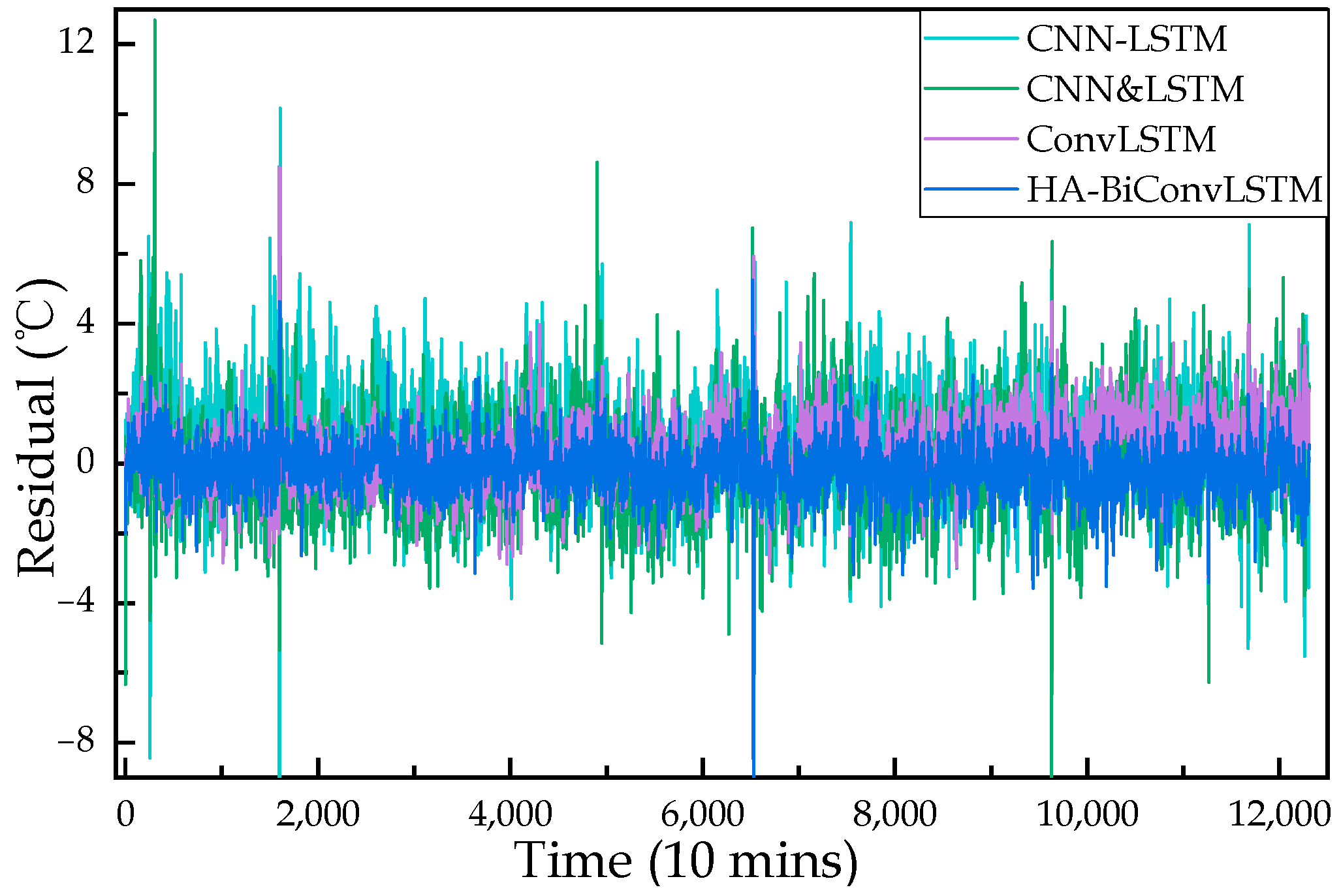
We constructed a novel HA-BiConvLSTM spatio-temporal normal behavior model (NBM) for a wind turbine gearbox. Convolutional long short-term memory (ConvLSTM) perfectly integrates the powerful local spatial-feature extractive capability of CNN and the efficient time series processing capability of LSTM, the embedded network structure of which compensates disadvantages of conventional parallel or sequential structures (denoted as CNN-LSTM and CNN&LSTM) to some extent. Compared with CNN-LSTM and CNN&LSTM, the constructed HA-BiConvLSTM model achieved better valuation result in terms of RMSE, MAE, MAPE, and R² metrics.

(3)

We designed an improved EWMA-based dynamic anomaly detection approach. Based on the exponentially weighted moving-average algorithm (EWMA), the adaptive outlier thresholds of prediction residuals of different well-trained gearbox NBMs can be calculated to identify outliers. To reduce false alarms caused by some isolated outliers, an anomaly detection index, i.e., the outlier ratio within a sliding window, was proposed to improve the reliability of early gearbox faults. Results of the case study illustrated that the proposed HA-BiConvLSTM-iEWMA (HBCE) method can detect gearbox deteriorated conditions earlier than conventional CNN-LSTM and CNN&LSTM models, which verified the effectiveness, superiority, and robustness of the constructed HA-BiConvLSTM model.

The remainder of this paper is arranged as follows. Section 2 introduces the framework of the proposed HA-BiConvLSTM-iEWMA (HBCE) spatio-temporal condition monitoring method for wind turbine gearbox. Section 3 introduces the methodologies and structures of the constructed HA-BiConvLSTM gearbox normal behavior model. Section 4 introduces an improved EWMA-based dynamic anomaly detection approach. The proposed HBCE method is validated using actual gearbox oil over-temperature fault collected from a wind farm located in north China in Section 5, followed by brief conclusions in Section 6.

2. Framework of the Proposed HBCE Method

The framework of the proposed HA-BiConvLSTM-iEWMA (HBCE) condition monitoring method is depicted in Figure 1, which mainly contains two phrases: offline training and online monitoring.

Phase 1. Offline training.

Step 1. Data preprocessing. In order to eliminate outliers caused by turbulent wind, power curtailment, and sensor failure, the modified Thompson tau approach was used for the data cleaning of the original historical SCADA data to acquire a health modeling dataset. Additionally, data normalization needs to be implemented to reduce the difficulty of model training and shorten training time.

Step 2. Variable selection. Generally, when there are no limitations on computational resources and model complexity, the more input variables there are, the more likely it is to obtain a model with higher performance. However, to balance model complexity with model performance, a compound correlation analysis approach consisting of Pearson, Spearman, Kendall correlation coefficients was employed to select model input variables that have high correlation with model output.

Step 3. Data matrices for modeling. Sliding window approach was employed to process the selected model input variables to acquire modeling data matrices D, which were further split into train set ${\mathrm{D}}_{\mathrm{t}\mathrm{r}\mathrm{a}\mathrm{i}\mathrm{n}}$ and test set ${\mathrm{D}}_{\mathrm{t}\mathrm{e}\mathrm{s}\mathrm{t}}$ for model training and test.

Step 4. HA-BiConvLSTM model training and test. Based on train set ${\mathrm{D}}_{\mathrm{t}\mathrm{r}\mathrm{a}\mathrm{i}\mathrm{n}}$ and test set ${\mathrm{D}}_{\mathrm{t}\mathrm{e}\mathrm{s}\mathrm{t}}$ obtained in Step 3, the constructed HA-BiConvLSTM model in this study can be trained and tested to learn the behavior modes of a wind turbine gearbox when operating under health conditions.

Phase 2. Online monitoring.

Step 5. Predictions and prediction residuals of HA-BiConvLSTM. Based on the online SCADA data and the well-trained HA-BiConvLSTM model, real-time predictions of wind turbine gearbox temperature can be generated, and prediction residuals between the predictions and measurements can be calculated.

Step 6. Condition monitoring and fault alarm. To reduce false alarm caused by some isolated outlier, the exponentially weighted moving-average algorithm was used to smooth residual sequence and calculate the upper limit of the control chart UCL as adaptive outlier threshold to identify anomaly conditions. Then, the outlier ratio was computed within a sliding window as an anomaly detection index to determine whether to issue early fault alarm signals.

3. Constructed HA-BiConvLSTM Model

3.1. Data Preprocessing

3.1.1. Data Cleaning

Generally, the supervisory control and data acquisition (SCADA) system has been widely deployed in modern large-scale wind turbines regardless of online or offline wind farms, which can record and store massive high-dimensional and multi-source heterogeneous operation data of wind turbine key components, as well as environmental information around wind turbines. However, original historical SCADA data often contain outliers caused by turbulent wind, power curtailment, and sensor failure, which need to be eliminated to achieve health SCADA data for modeling.

In this study, the modified Thompson tau approach, which is a statistical method for deciding whether to keep or discard suspected outliers in a sample of a single variable, was employed for data cleaning using wind speed and active power of wind turbines. As for the wind speed and active power data, first divide the wind speed range into 0.5 m/s contiguous bins centered on multiples of 0.5 m/s, and then group the active power data into wind speed intervals (i.e., bins).

Mathematically, for the increasing ordered active power dataset $P_{\mathrm{i}}=\{p_{i, 1}, p_{i, 2}, \dots , p_{i, n}\}$ of the ith wind speed bin, where $i=1, 2, \dots , m$, $p_{i, 1}\le p_{i, 1}\le \cdots \le p_{i, n}$, m represents the number of wind speed bins, n stands for the number of active power samples in each wind speed bin, the mean ${\overline{p}}_i$ and standard deviation $S_i$ of $P_i$ can be calculated according to Equations (1) and (2).

$${\overline{p}}_i=\frac{1}{n}\sum _{j=1}^n{p}_{i, j}$$

(1)

$$S_i=\sqrt{\frac{1}{n}\sum _{j=1}^n\left(p_{i, j}-{\overline{p}}_i\right)}$$

(2)

Then, for an active power sample $p_{i, j}$, the absolute error ${\delta }_{i, j}$ can be calculated through Equation (3).

$${\delta }_{i, j}=\left|p_{i, j}-{\overline{p}}_i\right|$$

(3)

Generally, the larger the absolute error ${\delta }_{i, j}$, the more likely active power sample $p_{i, j}$ is to be a suspected outlier. Typically, either the first or last active power samples are most suspected, since they are the lowest and highest values of $P_i$, respectively.

Furthermore, the value of the modified Thompson tau $\tau$, which is a function of the number of active power samples (i.e., n), can be calculated by Equation (4).

$$\tau =\frac{t_{\alpha /2}\left(n-1\right)}{\sqrt{n\left(n-2+t_{\alpha /2}^2\right)}}$$

(4)

where $t_{\alpha /2}$ is the critical student’s t value, $\alpha$ refers to significance level and is set as $\alpha =0.01$ in this study.

The outlier detection strategy is as follows:

If ${\delta }_{i, j}>\tau S_i$, remove the active power sample. It is an outlier.

If ${\delta }_{i, j} \le \tau S_i$, keep the active power sample. It is not an outlier.

One suspected outlier is detected and eliminated at each time, and the mean ${\overline{p}}_i$ and standard deviation $S_i$ of $P_i$ will be recalculated. The process will be repeated until no more outliers are detected.

3.1.2. Data Normalization

SCADA data have multi-source heterogeneous characteristics and the values of different monitoring variables vary in size. To eliminate the impact of different variables’ dimensions on model training and to reduce the difficulty of model training, it is necessary to carry out data normalization to scale down the data range to [0, 1] according to Equation (5).

$$x^{\prime }=\frac{x-x_{min}}{x_{max}-x_{min}}$$

(5)

where $x$ is the original data, $x^{\prime }$ is the normalized data, $x_{min}$ and $x_{max}$ are the minimum and maximum of dataset X, respectively.

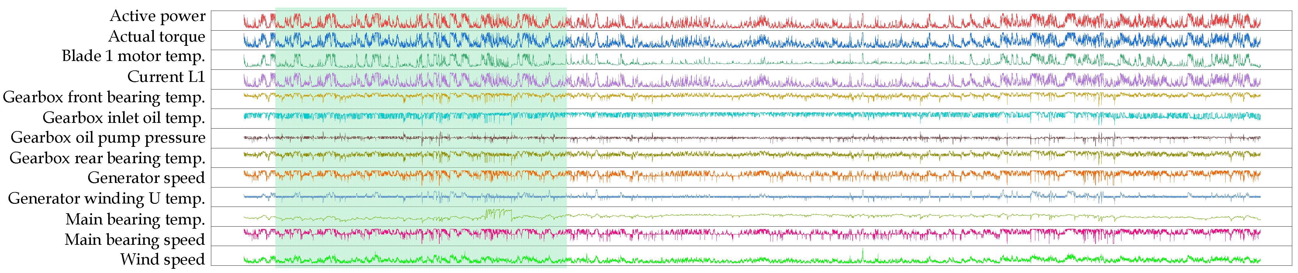
3.1.3. Variable Selection

The SCADA system records and stores hundreds of continuous or discrete operation condition parameters of wind turbine key components and environmental information around wind turbines. To reduce the complexity of the model and to improve the training efficiency, a hybrid correlation analysis approach was employed to select monitoring variables, which have high correlation with model output, as model inputs.

The hybrid correlation analysis designed in this study consists of three correlation coefficients, i.e., Pearson correlation coefficient $R_p$, Spearman correlation coefficient $R_s$, and Kendall correlation coefficient $R_k$, which can be calculated according to Equations (6)–(8), respectively.

$$R_p=\frac{{\sum }_{i=1}^N\left(x_i-\overline{x}\right)\left(y_i-\overline{y}\right)}{\sqrt{{\sum }_{i=1}^N(x_i-\overline{x}{)}^2}\sqrt{{\sum }_{i=1}^N(y_i-\overline{y}{)}^2}}$$

(6)

$$R_s=1-\frac{6{\sum }_{i=1}^N{d}_i^2(rank\left(x_i\right)-rank(y_i){)}^2}{N\left(N^2-1\right)}$$

(7)

$$R_k=\frac{{\sum }_{i<j}sign\left(\left(x_i-x_j\right)\left(y_i-y_j\right)\right)}{0.5N\left(N-1\right)}$$

(8)

where N represents the number of samples, $x_i$, $x_j$, $y_i$, $y_j$ represent the measurements, $\overline{x}$, $\overline{y}$ represent the average values of the measurements, d_i represents the difference between the two variables in ranks of the “ith” elements, rank (·) represents an order function, sign (·) represents a sign function.

Statistically, the absolute values of different correlation coefficients can quantitatively measure the correlation between variables, |R| < 0.3 indicates a weak correlation between variables; 0.3 < |R| < 0.7 indicates a moderate correlation between variables; and |R| > 0.7 indicates a strong correlation between variables. In this study, we directly chose 0.3 as the correlation threshold, based on which we carried out the variable selection procedure.

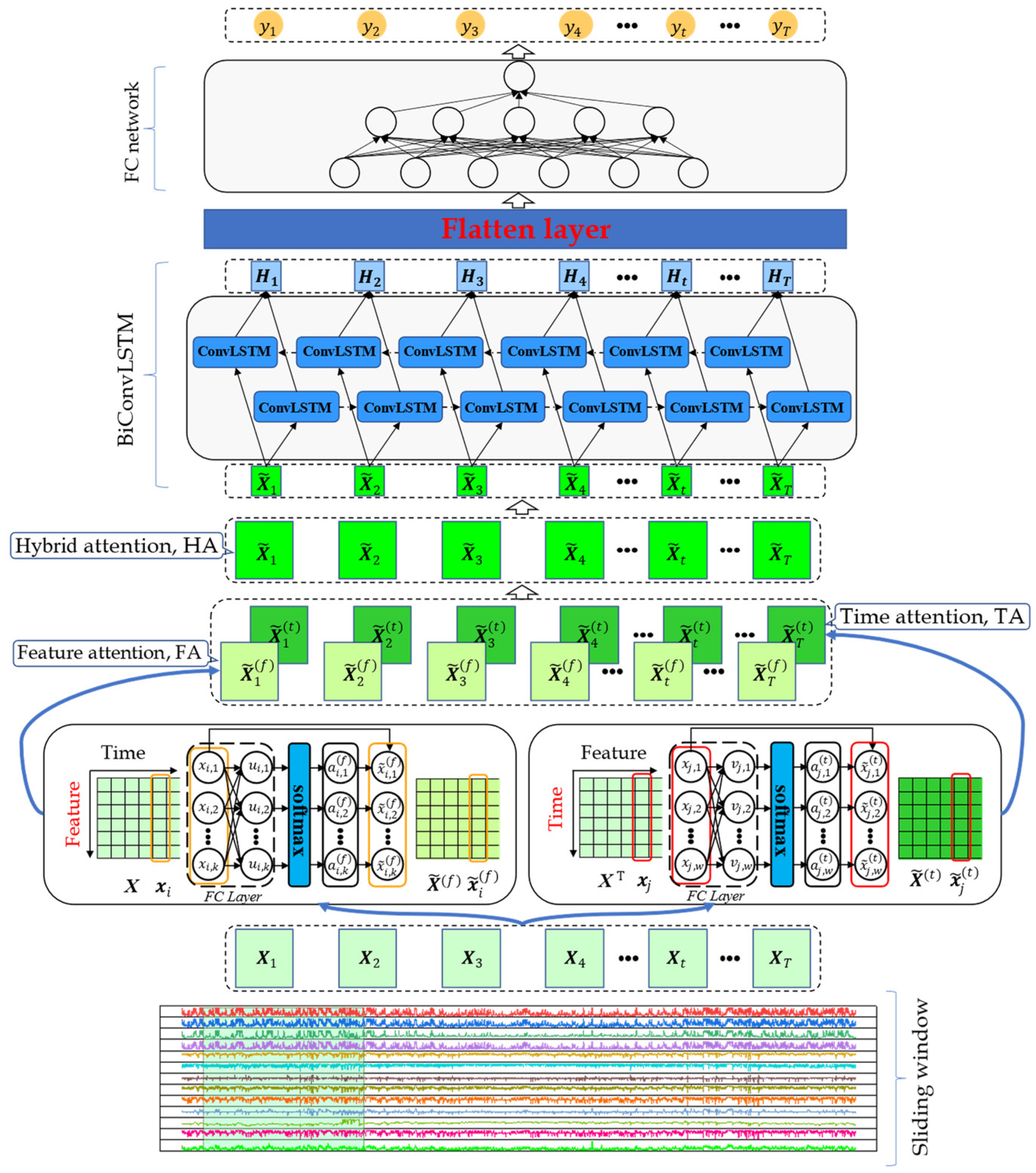
3.1.4. Model Input Matrices Based on the Sliding Window Algorithm

Additionally, prior to model training, the sliding window algorithm was employed to process the health modeling dataset obtained after data preprocessing and variable selection to acquire model input data matrices $X_1, X_2, X_3, \dots , X_n, \dots$ within windows. The brief data processing process of sliding window is displayed in Figure 2, and the nth model input matrix can be described as Equation (9).

$$\begin{array}{ll}{X}_n& =(x_1, x_2, \dots ,x_j, \dots , x_k{)}^T\\ & =\left(x_{\left(n-1\right)s+1}, x_{\left(n-1\right)s+2}, \dots ,x_{\left(n-1\right)s+i}, \dots , x_{\left(n-1\right)s+w}\right)\\ & =\left(\begin{array}{cccccc}{x}_{\left(n-1\right)s+1, 1}& x_{\left(n-1\right)s+2, 1}& \dots & x_{\left(n-1\right)s+i, 1}& \dots & x_{\left(n-1\right)s+w, 1}\\ x_{\left(n-1\right)s+1, 2}& x_{\left(n-1\right)s+2, 2}& \dots & x_{\left(n-1\right)s+i, 2}& \dots & x_{\left(n-1\right)s+w, 2}\\ \dots & \dots & \dots & \dots & \dots & \dots \\ x_{\left(n-1\right)s+1, j}& x_{\left(n-1\right)s+2, j}& \dots & x_{\left(n-1\right)s+i, j}& \dots & x_{\left(n-1\right)s+w, j}\\ \dots & \dots & \dots & \dots & \dots & \dots \\ x_{\left(n-1\right)s+1, k}& x_{\left(n-1\right)s+2, k}& \dots & x_{\left(n-1\right)s+i, k}& \dots & x_{\left(n-1\right)s+w, k}\end{array}\right)\end{array}$$

(9)

where s is the time step length of the sliding window, w is the width of the sliding window, k is the number of selected variables (i.e., model input features), $x_{\left(n-1\right)s+i}=(x_{\left(n-1\right)s+i, 1}, x_{\left(n-1\right)s+i, 2}, \dots , x_{\left(n-1\right)s+i, j}, \dots , x_{\left(n-1\right)s+i, k})$ represents the feature vector of the nth matrix at $\left(n-1\right)s+i$ time point, $x_j=(x_{\left(n-1\right)s+1, j}, x_{\left(n-1\right)s+2, j}, \dots , x_{\left(n-1\right)s+i, j}, \dots , x_{\left(n-1\right)s+w, j})$ represents the time series of the jth feature.

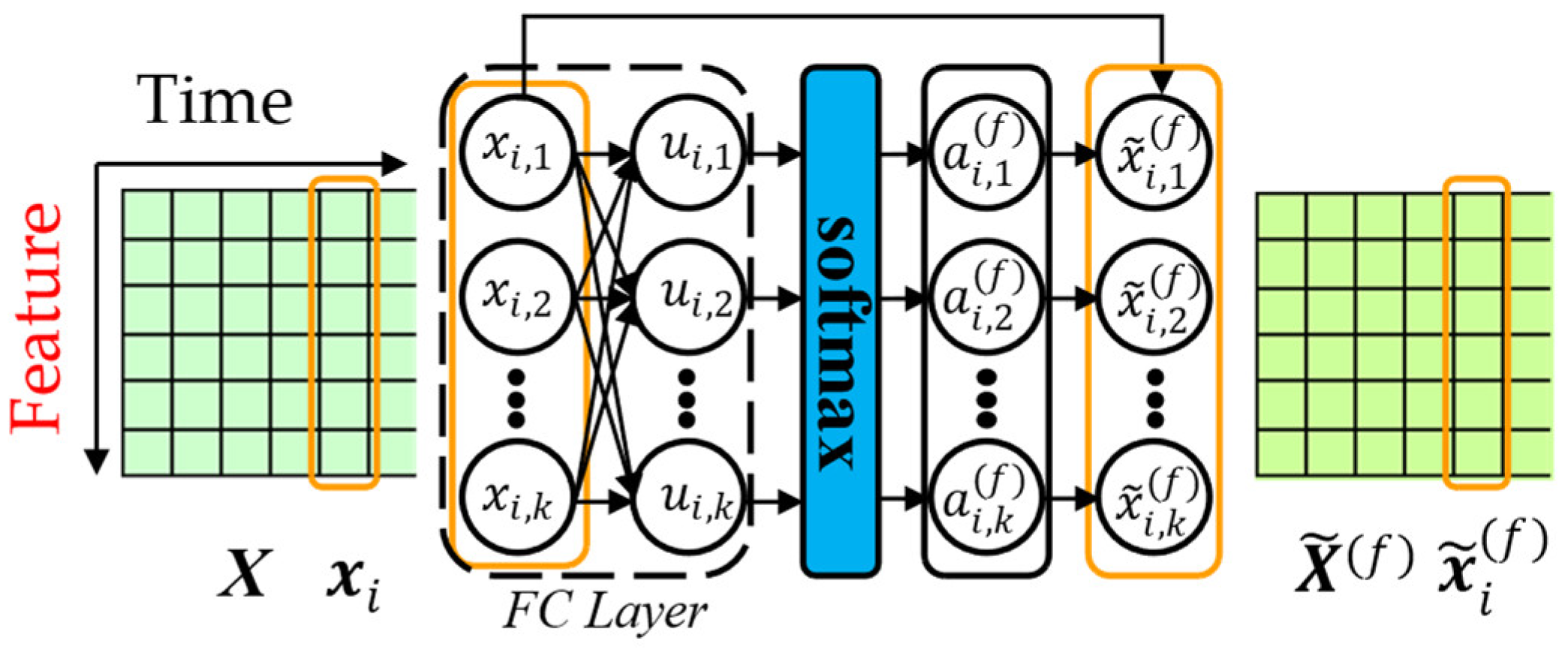
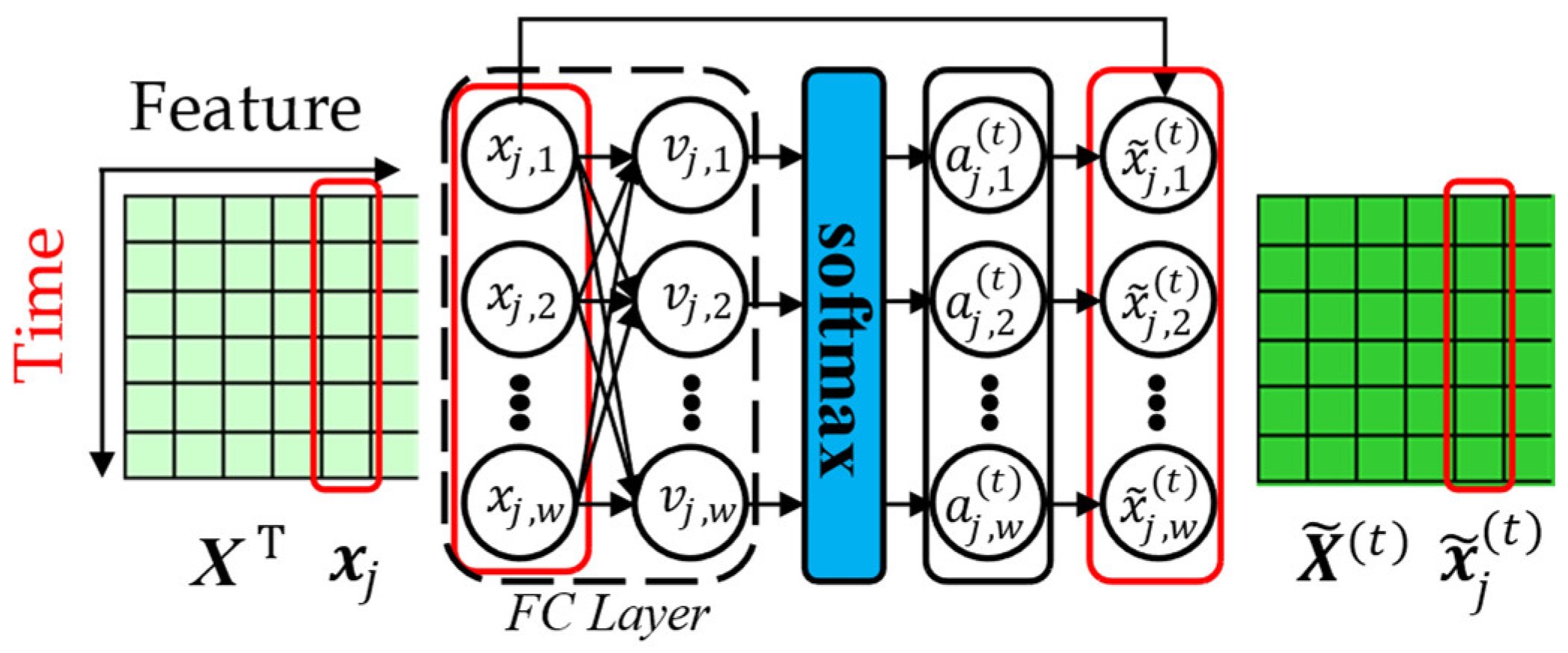
3.2. Spatio-Temporal Hybrid Attention Mechanism

Attention mechanisms originate from the study of human vision. The earliest application of attention mechanism in deep learning is Bahdanau attention proposed by Bahdanau et al. [40], which is used to solve the alignment problem of source languages with different lengths in machine translation. At present, attention mechanisms are widely used in natural language processing, speech recognition, and other aspects. As a resource allocation strategy, attention mechanisms can adaptively allocate attention weights to input information, enhance the model’s attention to key features, weaken or even discard redundant features, and ultimately achieve the goal of improving model performance. In this study, a hybrid attention mechanism consisting of feature attention and time attention was designed to allocate attention weights to model input matrices.

3.2.1. Feature Attention

The feature attention module focuses on the correlation between different input variables and the target variable from the spatial dimension, assigning higher weights to input variables with higher correlation. Based on the model input matrix X obtained by the sliding window algorithm, the calculation process of feature attention can be described as Figure 3.

Specifically, the original model input matrix X was fed into a one-hidden-layer fully connected network and a softmax-normalization layer to acquire the feature attention weights matrix $A^{\left(f\right)}$, which was further multiplied with X to achieve the feature attention weighted matrix ${\tilde{X}}^{\left(f\right)}$. The detailed mathematical calculation process is shown in Equations (10)–(14).

$$\begin{array}{ll}X& =\left(x_1, x_2, \dots ,x_i, \dots , x_w\right)\\ & =\left(\begin{array}{cccccc}{x}_{1, 1}& x_{2, 1}& \dots & x_{i, 1}& \dots & x_{w, 1}\\ x_{1, 2}& x_{2, 2}& \dots & x_{i, 2}& \dots & x_{w, 2}\\ \dots & \dots & \dots & \dots & \dots & \dots \\ x_{1, j}& x_{2, j}& \dots & x_{i, j}& \dots & x_{w, j}\\ \dots & \dots & \dots & \dots & \dots & \dots \\ x_{1, k}& x_{2, k}& \dots & x_{i, k}& \dots & x_{w, k}\end{array}\right)\end{array}$$

(10)

$$u_i=\sigma \left(W_f{x}_i+b_f\right)=(u_{i, 1}, u_{i, 2}, \dots ,u_{i, j}, \dots , u_{i, k}{)}^T$$

(11)

$${\tilde{x}}_{i, j}^{\left(f\right)}=a_{i, j}^{\left(f\right)}{x}_{i, j}=\frac{{\mathrm{e}\mathrm{x}\mathrm{p}(u}_{i, j})}{{\sum }_{j=1}^k{u}_{i, j}}{x}_{i, j}$$

(12)

$${\tilde{x}}_i^{\left(f\right)}=({\tilde{x}}_{i, 1}^{\left(f\right)}, {\tilde{x}}_{i, 2}^{\left(f\right)}, \dots , {\tilde{x}}_{i, j}^{\left(f\right)}, \dots , {\tilde{x}}_{i, k}^{\left(f\right)}{)}^T$$

(13)

$${\tilde{X}}^{\left(f\right)}=\left({\tilde{x}}_1^{\left(f\right)}, {\tilde{x}}_2^{\left(f\right)}, \dots , {\tilde{x}}_i^{\left(f\right)}, \dots , {\tilde{x}}_w^{\left(f\right)}\right)$$

(14)

where σ (.) is the Sigmoid activation function, $W_f$ is the weight matrix, $b_f$ is the bias vector, $u_{i, j}$ and $a_{i, j}^{\left(f\right)}$, respectively, represent the feature attention weights before and after the softmax normalization.

3.2.2. Time Attention

The time attention module focuses on the correlation between the measurements different historical time points and the current prediction from the temporal dimension, assigning higher weights to historical time points with higher correlation. Based on the model input matrix X obtained by the sliding window algorithm, the calculation process of time attention can be described as Figure 4.

Specifically, the original model input matrix X was fed into a one-hidden-layer fully connected network and a softmax-normalization layer to acquire the time attention weights matrix $A^{\left(t\right)}$, which was further multiplied with X to achieve the time attention weighted matrix ${\tilde{X}}^{\left(t\right)}$. The detailed mathematical calculation process is shown in Equations (15)–(19).

$$\begin{array}{ll}{X}^T& =\left(x_1, x_2, \dots ,x_j, \dots , x_k\right)\\ & =\left(\begin{array}{cccccc}{x}_{1, 1}& x_{2, 1}& \dots & x_{j, 1}& \dots & x_{k, 1}\\ x_{1, 2}& x_{2, 2}& \dots & x_{j, 2}& \dots & x_{k, 2}\\ \dots & \dots & \dots & \dots & \dots & \dots \\ x_{1, i}& x_{2, i}& \dots & x_{j, i}& \dots & x_{k, i}\\ \dots & \dots & \dots & \dots & \dots & \dots \\ x_{1, w}& x_{2, w}& \dots & x_{j, w}& \dots & x_{k, w}\end{array}\right)\end{array}$$

(15)

$$v_i=\sigma \left(W_t{x}_j+b_t\right)=(v_{j, 1}, v_{j, 2}, \dots ,v_{j, i}, \dots , v_{j, w}{)}^T$$

(16)

$${\tilde{x}}_{j, i}^{\left(t\right)}=a_{j, i}^{\left(t\right)}{x}_{j, i}=\frac{{\mathrm{e}\mathrm{x}\mathrm{p}(v}_{j, i})}{{\sum }_{i=1}^w{v}_{j, i}}{x}_{j, i}$$

(17)

$${\tilde{x}}_j^{\left(t\right)}=({\tilde{x}}_{j, 1}^{\left(t\right)}, {\tilde{x}}_{j, 2}^{\left(t\right)}, \dots , {\tilde{x}}_{j, i}^{\left(t\right)}, \dots , {\tilde{x}}_{j, w}^{\left(t\right)}{)}^T$$

(18)

$${\tilde{X}}^{\left(t\right)}=\left({\tilde{x}}_1^{\left(t\right)}, {\tilde{x}}_2^{\left(t\right)}, \dots , {\tilde{x}}_j^{\left(t\right)}, \dots , {\tilde{x}}_k^{\left(t\right)}\right)$$

(19)

where σ (.) is the Sigmoid activation function, $W_t$ is the weight matrix, $b_t$ is the bias vector, $v_{j, i}$ and $a_{j, i}^{\left(t\right)},$ respectively, represent the time attention weights before and after the softmax normalization.

3.2.3. Hybrid Attention

Based on the feature attention weighted matrix and the time attention weighted matrix, the hybrid attention weighted matrix can be calculated by Equation (20).

$$\tilde{X}={\tilde{X}}^{\left(s\right)} ⨀ ({\tilde{X}}^{\left(t\right)}{)}^T$$

(20)

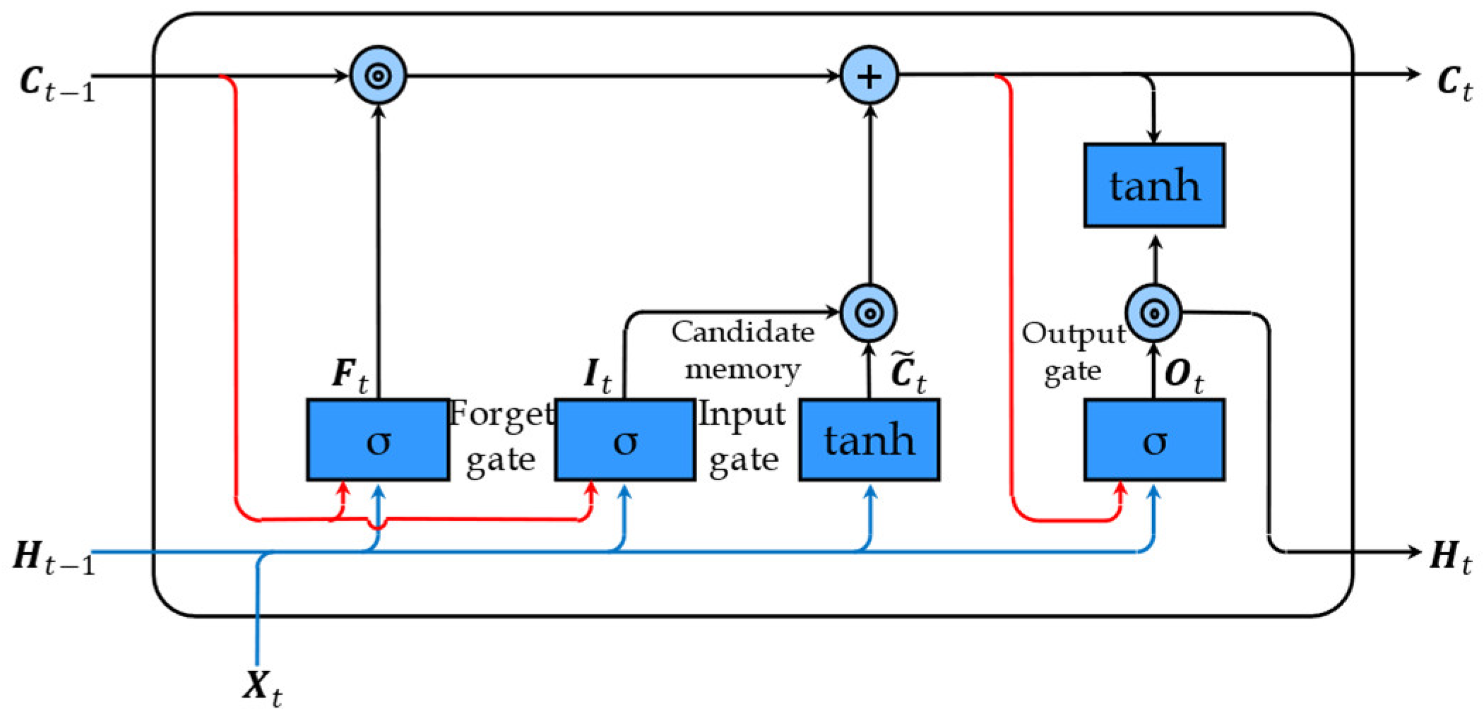
3.3. Bidirectional Conventional Long Short-Term Memory Network

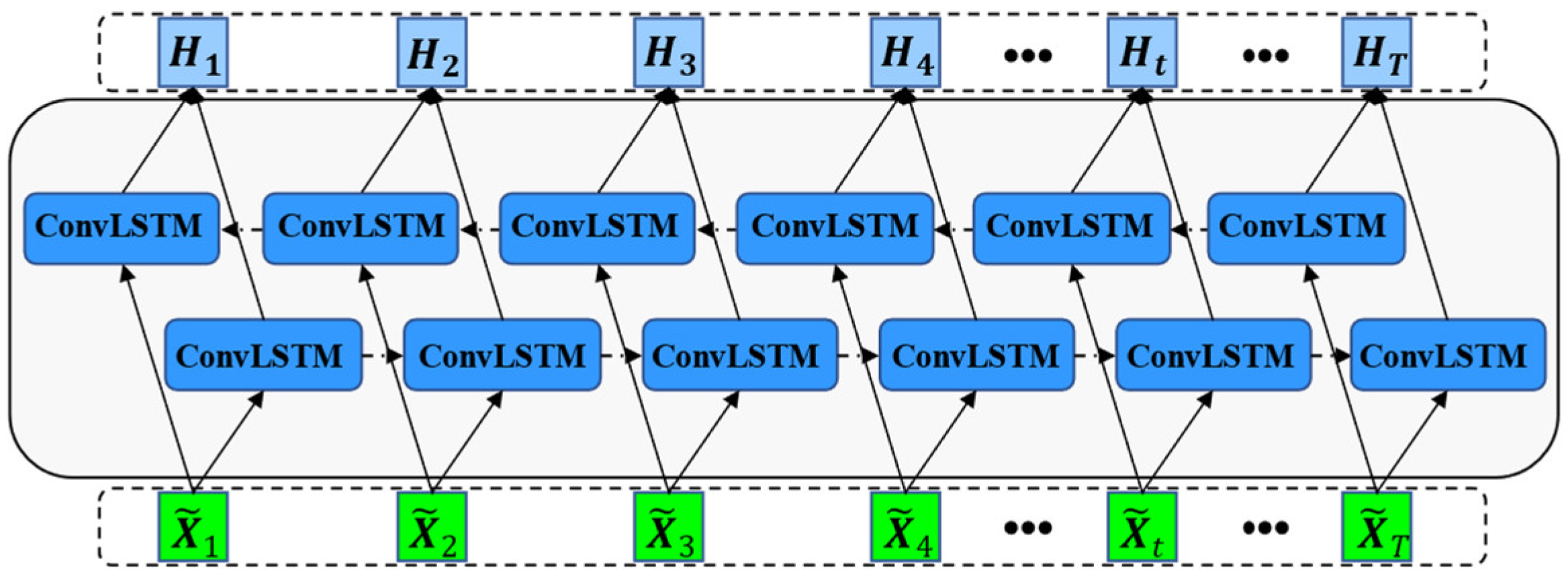
Recurrent neural networks (RNNs) are a family of neural networks with short-term memory capability, which are good at processing time series data. The neurons of recurrent neural networks can not only receive information from other neurons, but also from themselves, forming a network structure with loops. Recurrent neural networks have been widely used in speech recognition, language model, natural language generation and other tasks. The parameter learning of recurrent neural network can be learned according to the back-propagation through time (BPTT) algorithm [41], which can transfer the error information backward step by step in the reverse order of time. However, for the conventional recurrent neural network (RNN), when the input sequence is relatively long, there will be gradient explosion or gradient vanishing problems [42], also known as long-range dependence problems. In order to solve those problems, people have made many improvements to the conventional recurrent neural network, among which the most effective way is to introduce a gating mechanism.

3.3.1. ConvLSTM

Conventional long short-term memory network (ConvLSTM), proposed by Shi et al. [43] in 2015 for precipitation nowcasting, is an improved variant of the fully connected long short-term memory (FC-LSTM). Fully connected long short-term memory (FC-LSTM) is a variant of RNN, which takes one-dimensional sequential feature vectors as model input and calculates both the input-to-state and state-to-input transactions in the fully connected manner [44]. By replacing the fully connected operators with the convolution operators in the input-to-state and state-to-input transactions, the ConvLSTM network can possess the mining capabilities of local spatial features while learning the temporal feature hidden in model inputs. Additionally, different from traditional spatio-temporal models (i.e., CNN-LSTM and CNN&LSTM), which achieve both the spatial features and temporal features extraction capabilities by simply combining CNN and LSTM in sequential or parallel ways, the ConvLSTM network integrates CNN and LSTM in an embedded manner and has better spatiotemporal interaction and synchronization. The structure of the conventional long short-term memory unit is displayed in Figure 5.

As can be seen from Figure 5, compared with the conventional FC-LSTM unit, the improvements of ConvLSTM unit are to replace the fully connected operations by the convolutional operations (i.e., the blue lines of the structure of the ConvLSTM unit), which make it additionally possess the powerful capabilities of mining the spatial feature hidden in the input data matrices, except for effectively handling the temporal correlations.

The introduction of the gate mechanisms can make the convolutional long short-term networks (ConvLSTM) effectively address the problems of gradient disappearance or gradient explosion existed in the traditional deep recurrent neural networks. As can be seen from Figure 5, three gates—a forget gate that determines the information ratio that the memory cell $C_{t-1}$ needs to discard, an input gate that determines the information ratio that the candidate memory cell ${\tilde{C}}_t$ need to reserve, and an output gate that determines the information ratio that the memory cell $C_t$ need to pass to the hidden state $H_t$.

The input gate $I_t$, forget gate $F_t$, memory cell $C_t$, output gate $O_t$, and hidden state $H_t$ can be calculated according to Equations (21)–(25).

$$I_t=\sigma \left(W_{xi}\ast X_t+W_{hi}\ast H_{t-1}+W_{ci }⨀{ C}_{t-1}+b_i\right)$$

(21)

$$F_t=\sigma \left(W_{xf}\ast X_t+W_{hf}\ast H_{t-1}+W_{cf} ⨀ C_{t-1}+b_f\right)$$

(22)

$$C_t=F_t ⨀{ C}_{t-1}+I_{t }⨀ \tanh \left(W_{xc}\ast X_t+W_{hc}\ast H_{t-1}+b_c\right)$$

(23)

$$O_t=\sigma \left(W_{xo}\ast X_t+W_{ho}\ast H_{t-1}+W_{co }⨀ C_t+b_o\right)$$

(24)

$$H_t=O_t ⨀ \mathrm{t}\mathrm{a}\mathrm{n}\mathrm{h}\left(C_t\right)$$

(25)

where $\ast$ represents the convolution operator, $⨀$ represents the Hadamard product.

3.3.2. BiConvLSTM

The bidirectional conventional long short-term memory network (BiConvLSTM) is composed of two ConvLSTM networks with identical structures and opposite propagation directions, namely, the forward layer and the backward layer. The structure of the BiConvLSTM network is displayed in Figure 6. Compared with ConvLSTM, BiConvLSTM inherits its many advantages and can also capture sequence information in both positive and negative directions.

Assuming that the forward and backward hidden states of the BiConvLSTM network can be denoted as ${\overrightarrow{H}}_t$ and ${\overleftarrow{H}}_t$, respectively, the update of both two-direction hidden states can be calculated by Equations (26) and (27).

$${\overrightarrow{H}}_t=\varnothing \left({\overrightarrow{W}}_{xh}{X}_t+{\overrightarrow{W}}_{hh}{\overrightarrow{H}}_{t-1}+{\overrightarrow{b}}_h\right)$$

(26)

$${\overleftarrow{H}}_t=\varnothing \left({\overleftarrow{W}}_{xh}{X}_t+{\overleftarrow{W}}_{hh}{\overleftarrow{H}}_{t+1}+{\overleftarrow{b}}_h\right)$$

(27)

where ${\overrightarrow{W}}_{xh}$, ${\overleftarrow{W}}_{xh}$, ${\overrightarrow{W}}_{hh}$, ${\overleftarrow{W}}_{hh}$ are weight parameter matrices, ${\overrightarrow{b}}_h$, ${\overleftarrow{b}}_h$ are bias parameter vectors.

Then, the hidden state ${\tilde{H}}_t$ can be achieved by concatenating the forward and backward hidden states, as shown by Equation (28), and the output $H_t$ can be calculated by Equation (29).

$${\tilde{H}}_t=\left[{\overrightarrow{H}}_t,{\overleftarrow{H}}_t\right]$$

(28)

$$H_t=W_{ho}{\tilde{H}}_t+b_o$$

(29)

where $W_{ho}$ is the weight parameter matrix, $b_o$ is the bias parameter vector.

3.4. Structure of the Constructed HA-BiConvLSTM Model

In summary, based on the sliding window algorithm, hybrid attention mechanism (HA), and bidirectional convolutional long short-term memory network (BiConvLSTM), the structure of the constructed HA-BiConvLSTM model in this study is shown in Figure 7, which consists of the sliding window module, spatio-temporal hybrid attention network, BiConvLSTM network, flatten layer, and two-layer fully connected network.

3.5. Evaluation Metrics

In this study, four commonly used evaluation metrics, i.e., root mean square error (RMSE), mean absolute error (MAE), mean absolute percentage error (MAPE), and determination coefficient (R²), were employed to quantitatively evaluate model performance, which can be computed by Equations (30)–(33).

$$RMSE=\sqrt{\frac{1}{n}\sum _{i=1}^n(y_i-{\widehat{y}}_i{)}^2}$$

(30)

$$MAE=\frac{1}{n}\sum _{i=1}^n\left|y_i-{\widehat{y}}_i\right|$$

(31)

$$MAPE=\frac{1}{n}\sum _{i=1}^n\frac{\left|y_i-{\widehat{y}}_i\right|}{y_i}$$

(32)

$$R^2=1-\frac{{\sum }_{i=1}^n(y_i-{\widehat{y}}_i{)}^2}{{\sum }_{i=1}^n(y_i-{\overline{y}}_i{)}^2}$$

(33)

where $y_i$, ${\widehat{y}}_i$, ${\overline{y}}_i$ stand for the measurements, predictions, and the mean of measurements, respectively.

4. Condition Monitoring

Based on the historical health SCADA data, the constructed HA-BiConvLSTM normal behavior model (NBM) for a wind turbine gearbox can be trained and tested. The well-trained HA-BiConvLSTM model can be further employed to carry out condition monitoring to identify early anomalies through online SCADA data. Generally, the predicted residuals between the real measurements and the predictions of NBMs are small with stable fluctuations around zero when the wind turbine operates under health conditions. However, once the wind turbine gearbox suffers from condition deterioration, the predicted residuals will slowly increase and fluctuate violently. Therefore, whether the operating conditions of the gearbox is normal or abnormal can be determined by real-time monitoring of the change trend of residuals, and further statistical analysis for the ratio of outliers can be used to judge whether to trigger the early fault alarms.

In this study, an improved exponentially weighted moving-average algorithm (iEWMA) based anomaly detection approach was designed for gearbox condition monitoring. Specifically, based on EWMA algorithm, the adaptive outlier threshold of prediction residuals is firstly calculated to identify outliers, then a further statistical analysis of the outlier ratio within a sliding window is conducted to reduce false alarms caused by some isolated outliers.

According to the original predicted residual $r_t$ as shown by Equation (34), the EWMA-smoothed residual $e_t$ can be calculated by Equation (35).

$$r_t=y_t-{\widehat{y}}_t$$

(34)

$$e_t=(1-\lambda )e_{t-1}+\lambda r_t=(1-\lambda {)}^t{e}_0+\lambda \sum _{k=0}^{t-1}(1-\lambda {)}^k{r}_{t-k}$$

(35)

where $y_t$, ${\widehat{y}}_t$ are the measurements and predictions, respectively, $\lambda \in \left(0,1\right]$ represents the smoothing coefficient. The larger the smoothing coefficient $\lambda$, the greater the weight of the current sample $r_t$. In this study, we set $\lambda =0.2$.

Then, the mean ${\mu }_{e_t}$ and standard deviation ${\sigma }_{e_t}$ of the EWMA-smoothed residual $e_t$ can be calculated by Equations (36) and (37), respectively.

$${\mu }_{e_t}={\mu }_{r_t}$$

(36)

$${{\sigma }_{e_t}}^2=\frac{\lambda [1-(1-\lambda {)}^{2t}]}{\left(2-\lambda \right)n_s}{{\sigma }_{r_t}}^2$$

(37)

where ${\mu }_{r_t}$ represents the mean of the original residuals, ${\sigma }_{r_t}$ represents the standard deviation of the original residuals, $n_s$ is the number of residual samples.

The upper limit of the EWMA control chart $U_{CL}\left(t\right)$ can be further calculated by Equation (38) and used as an adaptive outlier threshold to identify anomaly conditions (i.e., when residual exceeding $U_{CL}\left(t\right)$) of the wind turbine gearbox.

$$U_{CL}\left(t\right)={\mu }_{e_t}+\gamma {\sigma }_{e_t}={\mu }_{r_t}+\gamma {\sigma }_{r_t}\sqrt{\frac{\lambda [1-(1-\lambda {)}^{2t}]}{\left(2-\lambda \right)n_s}}$$

(38)

where $\gamma$ is a constant and set as 3 in this study.

Additionally, an outlier ratio $\eta$ within a sliding window was defined to reduce false alarms caused by some isolated outliers, as shown by Equation (39).

$$\eta =\frac{N_{outlier}}{N_{window}}$$

(39)

where $N_{outlier}$ and $N_{window}$ represent the number of outliers and the number of all residual samples within a sliding window, respectively. In this study, the window width was set as 6.

5. Case Study

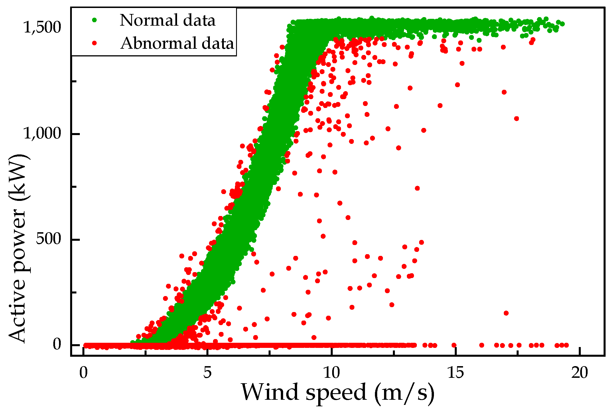
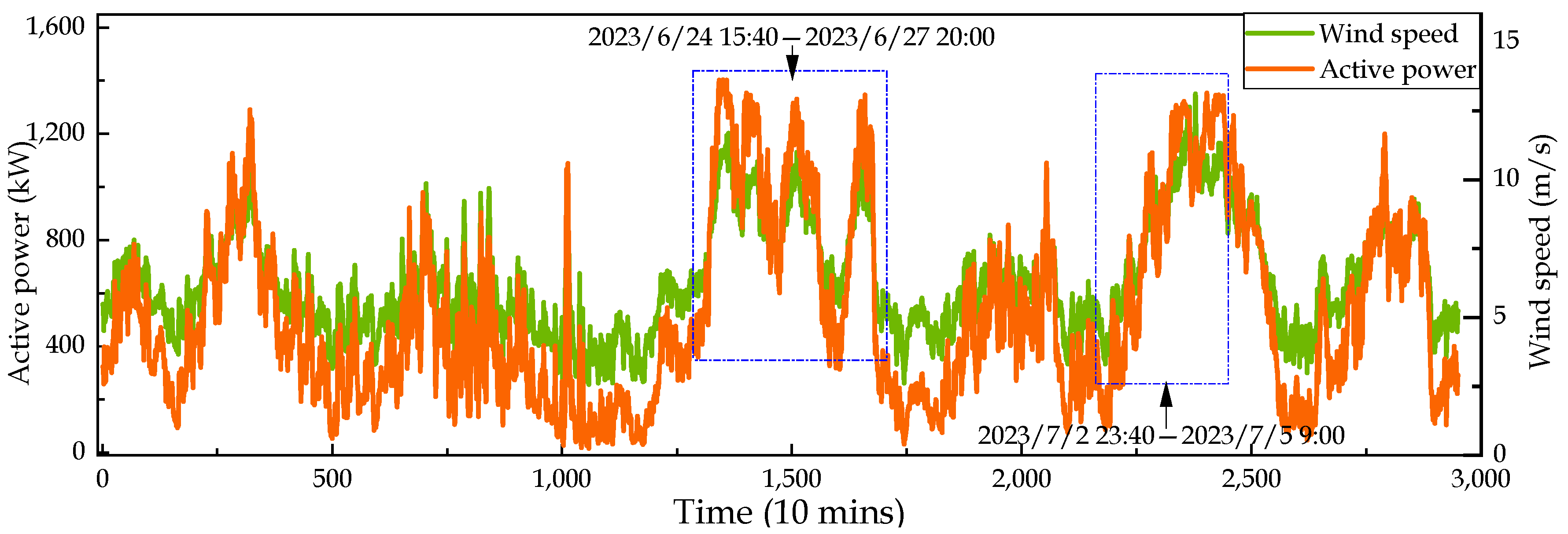
5.1. Data Description

In this study, the health dataset H acquired from the double-fed induction wind turbine WT #23 of a wind farm located in north China was used to train and test different normal behavior models (NBMs), which include the constructed HA-BiConvLSTM model and the traditional CNN-LSTM and CNN&LSTM spatio-temporal models. The fault dataset F collected from WT #17, which experienced a gearbox oil over-temperature fault on 5 July 2023 at 9:00, was employed to verify early fault detection capabilities of different NBMs by carrying out condition monitoring on WT #17. Detailed information about the health dataset H and fault dataset F is listed in

Table 1. Detailed information of health and fault datasets for modeling.

Dataset	WT Number	Time Range	Data Size	Fault Time	Fault Type
Health dataset H	#23	1 January 2020–31 December 2020	51,451	——	——
Fault dataset F	#17	10 June 2020–11 July 2020	2983	5 July 2023 9:00	Gearbox oil overtemperature

.

5.2. Data Preprocessing

Based on the modified Thompson tau approach described in Section 3.1.1, data cleaning can be implemented on the original health dataset H to acquire modeling dataset M, which will be further split by 0.7:0.3 to obtain train set A and test set B.

Table 2. Results of data cleaning and data splitting.

Original Health Dataset	Model Dataset	Train Set	Test Set
51,451	43,167	30,217	12,950

lists the detailed results of data cleaning and data splitting, and Figure 8 visually displays the results of data cleaning.

Moreover, to decrease the NBMs’ training difficulty and enhance the NBMs’ training speed, SCADA monitoring variables need to carry out data normalization according to Equation (5).

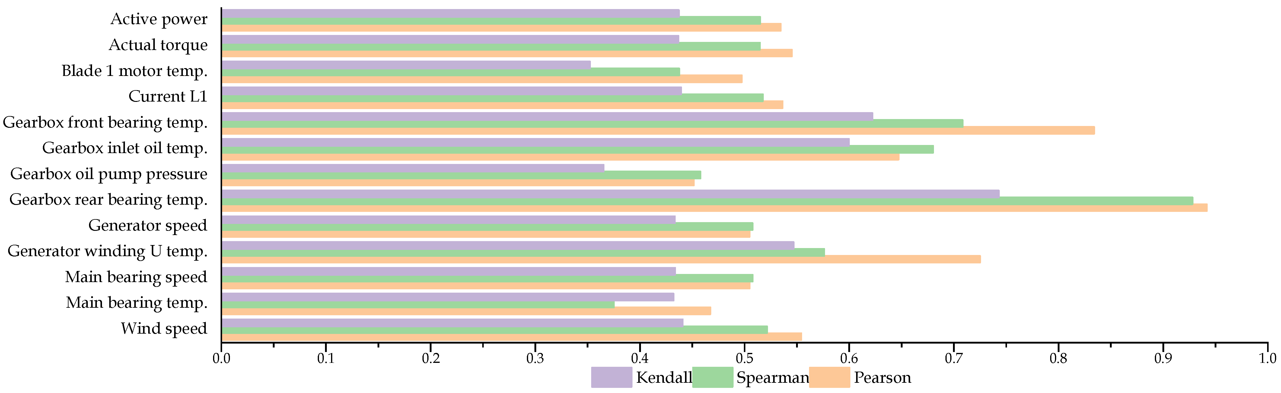
5.3. Variable Selection

To reduce the model complexity, based on the variable selection method described in Section 3.1.3, the hybrid correlation analysis including Pearson, Spearman, and Kendall correlation coefficients was performed on numerous SCADA monitoring variables to select variables that had higher correlations with the model output as the model inputs. In this study, comprehensively considering the correlation analysis result and wind turbine operation control principle, we selected 13 variables with correlation coefficients greater than 0.3 (i.e., active power, actual torque, blade 1 motor temperature, current L1, gearbox front bearing temperature, gearbox inlet oil temperature, gearbox oil pump pressure, gearbox rear bearing temperature, generator speed, generator winding U temperature, main bearing temperature, main bearing speed, wind speed) as the model inputs, gearbox oil temperature as the model output. It should be noted that for variables like currents (L1, L2, L3) and generator winding temperature (U, V, W), we only chose one phase as the model input. Detailed calculation results of three correlation coefficients are shown in Figure 9.

5.4. Model Train and Test

Based on the train set A and test set B acquired in Section 5.2, the constructed HA-BiConvLSTM model and three other comparative models (i.e., CNN-LSTM, CNN&LSTM, ConvLSTM) were trained and tested. In this study, the mean square error (MSE) loss was used to training the constructed model, and the learning rate, the batch size, the number of epochs were set as 0.001, 64, 1000, respectively. The quantitative evaluation metrics (i.e., RMSE, MAE, MAPE, R²) of prediction residuals of different well-trained gearbox normal behavior models for the test set B are listed in

Table 3. Evaluation results of different NBMs.

Model	RMSE	MAE	MAPE	R2
CNN-LSTM	1.5003	1.1395	0.0196	0.9533
CNN&LSTM	1.3537	1.0252	0.0176	0.9669
ConvLSTM	0.9759	0.7471	0.0129	0.9814
HA-BiConvLSTM	0.7683	0.5696	0.0098	0.9918

.

As can be observed from Table 3, compared with CNN-LSTM and CNN&LSTM, the ConvLSTM model presented better performance with lower RMSE, MAE, and MAPE values and a higher R² value, obtaining the RMSE, MAE, MAPE reductions by about 31.61%, 30.97%, and 30.79% and the R2 improvement by 2.22% on average. The possible reason behind those may be that the special embedded network structure of ConvLSTM perfectly overcome the disadvantages of the non-interactive problem caused by the CNN&LSTM parallel network structure, or the non-synchronous problem caused by the CNN-LSTM cascaded network structure, which means that it can effectively mine the spatial-temporal features inherent in the massive high-dimensional SCADA time series.

Among all four comparative models, the constructed HA-BiConvLSTM model possessed the best prediction performance, due to the bidirectional network structure that can capture the sequential information from both forward and backward directions simultaneously, and the hybrid-attention introduction that can adaptively assign attention weights to input variables to enhance the model’s focus on key features or weaken the redundant features. The RMSE, MAE, and MAPE values of the HA-BiConvLSTM networks were 0.7683 °C, 0.5696 °C, and 0.0098, which were 21.27%, 23.75%, and 23.97% lower than those of the ConvLSTM network, respectively. The R² value of the HA-BiConvLSTM network was 0.9918, which was 1.06% higher than that of the ConvLSTM network.

Figure 10, Figure 11 and Figure 12 intuitively display the timing diagrams of prediction residuals of different models for test set B, the probability density distributions (PDF) of prediction residuals of different models for test set B, and the gearbox oil temperature predictions of different models for partial test set B, respectively.

As can be seen from Figure 10, Figure 11 and Figure 12, compared with CNN-LSTM and CNN&LSTM, the prediction results clearly illustrated the ConvLSTM’s advantages of smaller residual values, less residual outliers, more stable residual fluctuations, sharper probability density function (PDF) curve, and predictions closer to the real measurements, which verify the superiority of the network structure of ConvLSTM as a gearbox normal behavior model. It can be also found that the introduction of hybrid-attention and bidirectional-structure improved the model performance of ConvLSTM, and the constructed HA-BiConvLSTM model of this study performed best in all aspects (i.e., smallest residual values, sharpest PDF curve, and closest to the real measurements), which was consistent with the quantitative evaluation results in terms of RMSE, MAE, MAPE, and R² values, as listed in Table 3.

Overall, from both a quantitative metric and qualitative display perspective, the above-mentioned results listed in Table 3 and displayed in Figure 10, Figure 11 and Figure 12 verified the effectiveness and superiority of the constructed HA-BiConvLSTM model due to its powerful spatio-temporal feature mining ability, as a normal behavior model for a gearbox.

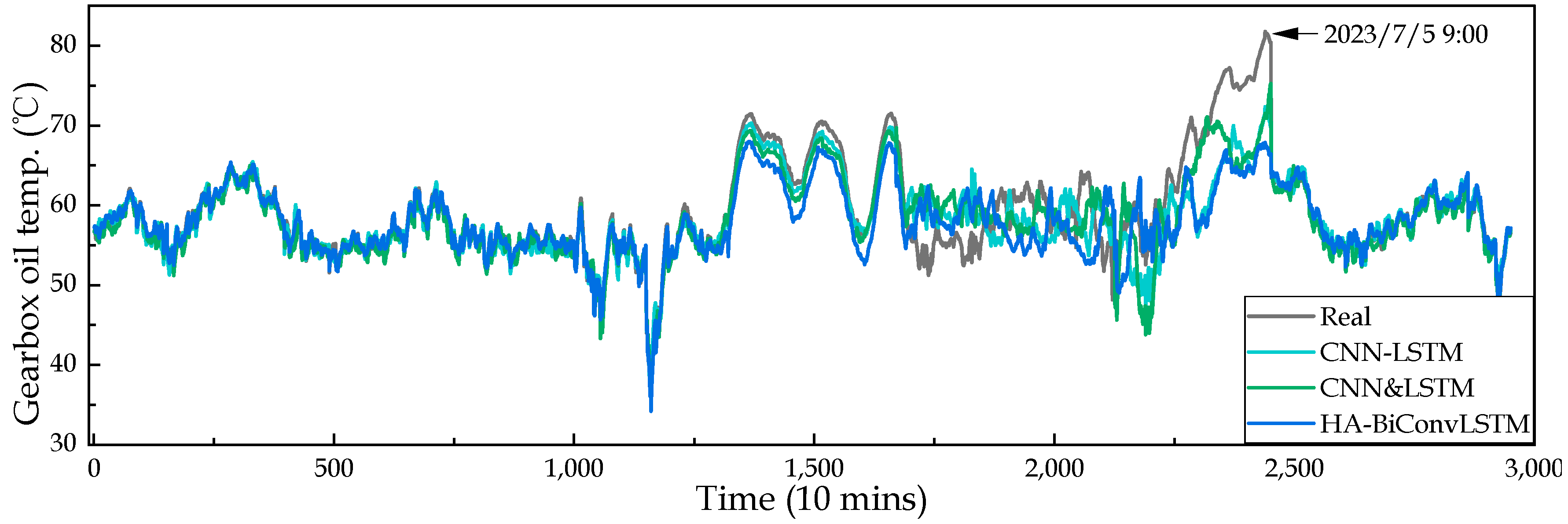
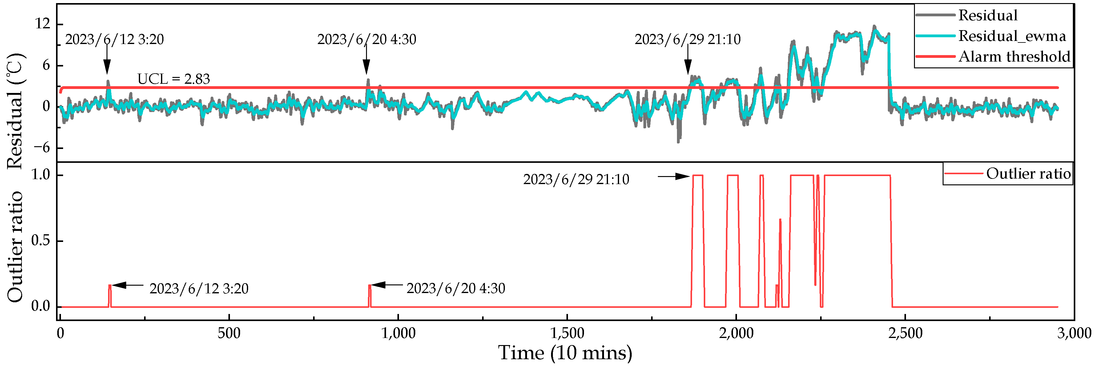
5.5. Condition Monitoring

When model offline training is completed, the well-trained HA-BiConvLSTM normal behavior model can be employed to implement online condition monitoring for a wind turbine gearbox. Generally, when a wind turbine operates normally, the NBMs prediction residuals would be small with stable fluctuations. Nevertheless, when a wind turbine gearbox suffers from condition deteriorations, the NBMs prediction residuals would be larger with violent fluctuations. Therefore, by real-time monitoring the change trend of the NBMs prediction residuals and residual statistical analysis using sliding windows, early faults of wind turbine gearboxes can be identified automatically in advance.

An actual gearbox fault case collected from a wind farm located in north China was used to verify the effectiveness of the proposed HBCE method for early fault detection. Meanwhile, to verify the superiority of the proposed HBCE method, conventional spatio-temporal models (i.e., CNN-LSTM, CNN&LSTM) were employed to compare and analyze the early fault detection results with the constructed HA-BiConvLSTM model. According to the alarm records of the SCADA system and the operation and maintenance logs of wind farm, WT #17 experienced a gearbox oil over-temperature fault on 5 July 2023 at 9:00. Approximate one month SCADA data around 5 July 2023 9:00 were selected for the validation analysis of the model’s early anomaly capability.

Figure 13 displays the wind speed and active power of WT #17, from which it can be found that the wind speed fluctuated violently between 5.4 m/s and 11.69 m/s during the period from 24 June 2023 15:40 to 27 June 2023 20:00, and gradually climbed from 3.31 m/s to the maximum 13.12 m/s during the period from 2 July 2023 23:40 to 5 July 2023 9:00.

Figure 14 displays the real measurements and different NBMs’ predictions of WT #17 gearbox oil temperature.

As can be observed in Figure 14, at beginning of the period, different NBMs’ predictions are very close to real measurements and consistent with the variation trend of real gearbox oil temperature. However, from around 24 June 2023, prediction residuals that indicate differences between predictions and measurements start to increase little by little with bigger fluctuations, and the consistencies of predictions and measurements also gradually deteriorate until the real gearbox oil temperature exceeds 80 °C on 5 July 2023 at 9:00.

Then, different NBMs’ prediction residuals can be calculated by predictions and measurements and smoothed by the exponentially weighted moving-average (EWMA) method, which can be further employed to calculate adaptive outlier thresholds by Equation (38). Then, through statistical analysis of outliers using sliding windows, early fault alarm can be triggered if the number of outliers in the window exceeds 6 (i.e., gearbox abnormal condition lasting for more than one hour). In this study, we set the window range as 6 and an alarm signal will be issued if the outlier ratio reaches 1.

For the fault dataset acquired from WT #17, which experienced a gearbox oil over-temperature fault, the original prediction residuals, smoothed residuals, adaptive thresholds, and outlier sliding window statistical results of three contrastive NBMs (i.e., the constructed HA-BiConvLSTM model in this study, the conventional spatio-temporal models CNN-LSTM and CNN&LSTM) are displayed in Figure 15, Figure 16 and Figure 17.

Figure 15 displays the condition monitoring results of the traditional CNN-LSTM model for WT #17.

As can be observed from Figure 15, during approximately the first half of the study period, the CNN-LSTM prediction residuals, including the original residual and the EWMA smoothed residual, were small with stable fluctuations; most residuals were under the adaptive outlier threshold UCL = 2.83 °C except for two isolated outliers on 12 June 2023 at 3:20 and 20 June 2023 at 4:30. However, from around 24 June 2023, prediction residuals started to gradually increase and fluctuate violently in amplitude until continuously exceeding the outlier threshold UCL = 2.83 °C around 29 June 2023 21:10, and the outlier ratio within a sliding window continuously reached the maximum 1 after 29 June 2023 21:10, which indicates that the CNN-LSTM model can identified the early fault signal 131.83 h in advance of the actual failure time 2023/7/5 9:00.

Figure 16 displays the condition monitoring results of the traditional CNN&LSTM model for WT #17.

As can be observed from Figure 16, the condition monitoring results of CNN&LSTM for WT #17 were similar to CNN-LSTM during approximately the first half of the study period, and most residuals were under the adaptive outlier threshold UCL = 2.62 °C, except for an isolated outlier on 18 June 2023 at 9:50. Moreover, within the second half-period, prediction residuals started to gradually increase and fluctuate violently in amplitude until continuously exceeding the outlier threshold UCL = 2.82 °C around 26 June 2023 5:30, and the outlier ratio within a sliding window continuously reached the maximum 1 after 26 June 2023 5:30, which indicates that the CNN&LSTM model can identified the early fault signal 219.5 h in advance of the actual failure time 5 July 2023 9:00.

Figure 17 displays the condition monitoring results of the constructed HA-BiConvLSTM model for WT #17.

As can be observed from Figure 17, different from the conventional CNN-LSTM and CNN&LSTM models, the prediction residuals of the constructed HA-BiConvLSTM model in this study did not include isolated outliers when the wind turbine gearbox operated under health conditions during approximately the first half-period, which illustrates the robustness of HA-BiConvLSTM. All residuals were below the outlier threshold UCL = 2.48 °C until continuously exceeding it around 24 June 2023 19:50, and the outlier ratio within a sliding window continuously reached the maximum 1 after 24 June 2023 19:50, which indicates that the HA-BiConvLSTM model can identify the early fault signal 253.17 h in advance of the actual failure time 5 July 2023 9:00.

In summary, through contrastively analyzing the condition monitoring results of different NBMs for fault wind turbine WT #17, the effectiveness, superiority, and robustness of the HA-BiConvLSTM model for wind turbine gearbox early fault detection were verified.

6. Conclusions

In this study, based on the hybrid attention mechanism (HA), the convolutional long short-term memory network (BiConvLSTM), and the improved exponentially weighted moving-average algorithm (iEWMA) based anomaly detection approach, we proposed a novel spatio-temporal condition monitoring method (HBCE) for a wind turbine gearbox. The effectiveness, superiority, and robustness of the proposed HBCE method was verified by the SCADA datasets collected from a wind farm in north China, and further compared with two conventional spatio-temporal models (i.e., CNN-LSTM and CNN&LSTM). The following conclusions can be drawn from the comparative experimental results.

(1)

The ConvLSTM model efficiently integrates CNN and LSTM through an embedded network structure, and overcomes the non-interactive or non-synchronous problems of conventional models when extracting spatio-temporal features. Compared with CNN-LSTM and CNN&LSTM, the ConvLSTM model presented better performance with lower RMSE, MAE, and MAPE values and a higher R² value.

(2)

The introduced hybrid attention mechanism can significantly enhance the model performance by calculating and assigning different attention weights from the spatio-temporal dimension for model input features. The constructed HA-BiConvLSTM model achieved the RMSE, MAE, and MAPE reductions by about 21.27%, 23.75%, and 23.97%, and the R² improvement by 1.06%, in comparison with the ConvLSTM model.

(3)

The proposed HBCE method has superior and robust early fault warning capabilities, which can efficiently identify early deteriorated conditions of a wind turbine gearbox 253.17 h in advance of the actual failure time, and 121.34 h, 33.67 h earlier than CNN-LSTM and CNN&LSTM.

In the future study, we will attempt to apply the proposed HBCE method to other different components (e.g., blade motor, main bearings, or generator) of wind turbines of the same or different type, to expand its application and evaluate its generalization.

References

1. Wang, J.; Liang, Y.; Zheng, Y.; Gao, R.X.; Zhang, F. An Integrated Fault Diagnosis and Prognosis Approach for Predictive Maintenance of Wind Turbine Bearing with Limited Samples. Renew. Energy 2020, 145, 642–650. [Google Scholar] [CrossRef]
2. Wang, Z.; Liu, C. Wind Turbine Condition Monitoring Based on a Novel Multivariate State Estimation Technique. Measurement 2021, 168, 108388. [Google Scholar] [CrossRef]
3. Park, J.; Kim, C.; Dinh, M.-C.; Park, M. Design of a Condition Monitoring System for Wind Turbines. Energies 2022, 15, 464. [Google Scholar] [CrossRef]
4. Zhu, Y.; Zhu, C.; Song, C.; Li, Y.; Chen, X.; Yong, B. Improvement of Reliability and Wind Power Generation Based on Wind Turbine Real-Time Condition Assessment. Int. J. Electr. Power Energy Syst. 2019, 113, 344–354. [Google Scholar] [CrossRef]
5. Zhu, Y.; Zhu, C.; Tan, J.; Wang, Y.; Tao, J. Operational State Assessment of Wind Turbine Gearbox Based on Long Short-Term Memory Networks and Fuzzy Synthesis. Renew. Energy 2022, 181, 1167–1176. [Google Scholar] [CrossRef]
6. Pérez-Pérez, E.-J.; López-Estrada, F.-R.; Puig, V.; Valencia-Palomo, G.; Santos-Ruiz, I. Fault Diagnosis in Wind Turbines Based on ANFIS and Takagi–Sugeno Interval Observers. Expert Syst. Appl. 2022, 206, 117698. [Google Scholar] [CrossRef]
7. Cho, S.; Choi, M.; Gao, Z.; Moan, T. Fault Detection and Diagnosis of a Blade Pitch System in a Floating Wind Turbine Based on Kalman Filters and Artificial Neural Networks. Renew. Energy 2021, 169, 1–13. [Google Scholar] [CrossRef]
8. Su, H.; Zhao, Y.; Wang, X. Analysis of a State Degradation Model and Preventive Maintenance Strategies for Wind Turbine Generators Based on Stochastic Differential Equations. Mathematics 2023, 11, 2608. [Google Scholar] [CrossRef]
9. Jiang, G.; Jia, C.; Nie, S.; Wu, X.; He, Q.; Xie, P. Multiview Enhanced Fault Diagnosis for Wind Turbine Gearbox Bearings with Fusion of Vibration and Current Signals. Measurement 2022, 196, 111159. [Google Scholar] [CrossRef]
10. Pandit, R.K.; Infield, D. SCADA-Based Wind Turbine Anomaly Detection Using Gaussian Process Models for Wind Turbine Condition Monitoring Purposes. IET Renew. Power Gener. 2018, 12, 1249–1255. [Google Scholar] [CrossRef]
11. Sun, P.; Li, J.; Wang, C.; Lei, X. A Generalized Model for Wind Turbine Anomaly Identification Based on SCADA Data. Appl. Energy 2016, 168, 550–567. [Google Scholar] [CrossRef]
12. Xie, T.; Xu, Q.; Jiang, C.; Lu, S.; Wang, X. The Fault Frequency Priors Fusion Deep Learning Framework with Application to Fault Diagnosis of Offshore Wind Turbines. Renew. Energy 2023, 202, 143–153. [Google Scholar] [CrossRef]
13. Zhang, J.; Xu, B.; Wang, Z.; Zhang, J. An FSK-MBCNN Based Method for Compound Fault Diagnosis in Wind Turbine Gearboxes. Measurement 2021, 172, 108933. [Google Scholar] [CrossRef]
14. Liu, X.; Guo, H.; Liu, Y. One-Shot Fault Diagnosis of Wind Turbines Based on Meta-Analogical Momentum Contrast Learning. Energies 2022, 15, 3133. [Google Scholar] [CrossRef]
15. López de Calle, K.; Ferreiro, S.; Roldán-Paraponiaris, C.; Ulazia, A. A Context-Aware Oil Debris-Based Health Indicator for Wind Turbine Gearbox Condition Monitoring. Energies 2019, 12, 3373. [Google Scholar] [CrossRef]
16. Fuentes, R.; Dwyer-Joyce, R.S.; Marshall, M.B.; Wheals, J.; Cross, E.J. Detection of Sub-Surface Damage in Wind Turbine Bearings Using Acoustic Emissions and Probabilistic Modelling. Renew. Energy 2020, 147, 776–797. [Google Scholar] [CrossRef]
17. Ma, Z.; Zhao, M.; Luo, M.; Gou, C.; Xu, G. An Integrated Monitoring Scheme for Wind Turbine Main Bearing Using Acoustic Emission. Signal Process. 2023, 205, 108867. [Google Scholar] [CrossRef]
18. Attallah, O.; Ibrahim, R.A.; Zakzouk, N.E. CAD System for Inter-Turn Fault Diagnosis of Offshore Wind Turbines via Multi-CNNs & Feature Selection. Renew. Energy 2023, 203, 870–880. [Google Scholar] [CrossRef]
19. Attallah, O.; Ibrahim, R.A.; Zakzouk, N.E. Fault Diagnosis for Induction Generator-Based Wind Turbine Using Ensemble Deep Learning Techniques. Energy Rep. 2022, 8, 12787–12798. [Google Scholar] [CrossRef]
20. Heydari, A.; Garcia, D.A.; Fekih, A.; Keynia, F.; Tjernberg, L.B.; De Santoli, L. A Hybrid Intelligent Model for the Condition Monitoring and Diagnostics of Wind Turbines Gearbox. IEEE Access 2021, 9, 89878–89890. [Google Scholar] [CrossRef]
21. Zhu, Y.; Zhu, C.; Tan, J.; Tan, Y.; Rao, L. Anomaly Detection and Condition Monitoring of Wind Turbine Gearbox Based on LSTM-FS and Transfer Learning. Renew. Energy 2022, 189, 90–103. [Google Scholar] [CrossRef]
22. McKinnon, C.; Carroll, J.; McDonald, A.; Koukoura, S.; Plumley, C. Investigation of Isolation Forest for Wind Turbine Pitch System Condition Monitoring Using SCADA Data. Energies 2021, 14, 6601. [Google Scholar] [CrossRef]
23. Tao, T.; Liu, Y.; Qiao, Y.; Gao, L.; Lu, J.; Zhang, C.; Wang, Y. Wind Turbine Blade Icing Diagnosis Using Hybrid Features and Stacked-XGBoost Algorithm. Renew. Energy 2021, 180, 1004–1013. [Google Scholar] [CrossRef]
24. Guo, P.; Fu, J.; Yang, X. Condition Monitoring and Fault Diagnosis of Wind Turbines Gearbox Bearing Temperature Based on Kolmogorov-Smirnov Test and Convolutional Neural Network Model. Energies 2018, 11, 2248. [Google Scholar] [CrossRef]
25. Wang, D.; Cao, C.; Chen, N.; Pan, W.; Li, H.; Wang, X. A Correlation-Graph-CNN Method for Fault Diagnosis of Wind Turbine Based on State Tracking and Data Driving Model. Sustain. Energy Technol. Assess. 2023, 56, 102995. [Google Scholar] [CrossRef]
26. Yang, W.; Liu, C.; Jiang, D. An Unsupervised Spatiotemporal Graphical Modeling Approach for Wind Turbine Condition Monitoring. Renew. Energy 2018, 127, 230–241. [Google Scholar] [CrossRef]
27. Wang, H.; Wang, H.; Jiang, G.; Wang, Y.; Ren, S. A Multiscale Spatio-Temporal Convolutional Deep Belief Network for Sensor Fault Detection of Wind Turbine. Sensors 2020, 20, 3580. [Google Scholar] [CrossRef]
28. Zhang, Z.; Wang, S.; Wang, P.; Jiang, P.; Zhou, H. Research on Fault Early Warning of Wind Turbine Based on IPSO-DBN. Energies 2022, 15, 9072. [Google Scholar] [CrossRef]
29. Jia, X.; Han, Y.; Li, Y.; Sang, Y.; Zhang, G. Condition Monitoring and Performance Forecasting of Wind Turbines Based on Denoising Autoencoder and Novel Convolutional Neural Networks; Social Science Research Network: Rochester, NY, USA, 2021. [Google Scholar]
30. Zhang, C.; Hu, D.; Yang, T. Anomaly Detection and Diagnosis for Wind Turbines Using Long Short-Term Memory-Based Stacked Denoising Autoencoders and XGBoost. Reliab. Eng. Syst. Saf. 2022, 222, 108445. [Google Scholar] [CrossRef]
31. Wu, Y.; Ma, X. A Hybrid LSTM-KLD Approach to Condition Monitoring of Operational Wind Turbines. Renew. Energy 2022, 181, 554–566. [Google Scholar] [CrossRef]
32. Li, G.; Wang, C.; Zhang, D.; Yang, G. An Improved Feature Selection Method Based on Random Forest Algorithm for Wind Turbine Condition Monitoring. Sensors 2021, 21, 5654. [Google Scholar] [CrossRef] [PubMed]
33. Xiao, X.; Liu, J.; Liu, D.; Tang, Y.; Qin, S.; Zhang, F. A Normal Behavior-Based Condition Monitoring Method for Wind Turbine Main Bearing Using Dual Attention Mechanism and Bi-LSTM. Energies 2022, 15, 8462. [Google Scholar] [CrossRef]
34. Xiang, L.; Wang, P.; Yang, X.; Hu, A.; Su, H. Fault Detection of Wind Turbine Based on SCADA Data Analysis Using CNN and LSTM with Attention Mechanism. Measurement 2021, 175, 109094. [Google Scholar] [CrossRef]
35. Pang, Y.; He, Q.; Jiang, G.; Xie, P. Spatio-Temporal Fusion Neural Network for Multi-Class Fault Diagnosis of Wind Turbines Based on SCADA Data. Renew. Energy 2020, 161, 510–524. [Google Scholar] [CrossRef]
36. Zhu, A.; Zhao, Q.; Yang, T.; Zhou, L.; Zeng, B. Condition Monitoring of Wind Turbine Based on Deep Learning Networks and Kernel Principal Component Analysis. Comput. Electr. Eng. 2023, 105, 108538. [Google Scholar] [CrossRef]
37. Kong, Z.; Tang, B.; Deng, L.; Liu, W.; Han, Y. Condition Monitoring of Wind Turbines Based on Spatio-Temporal Fusion of SCADA Data by Convolutional Neural Networks and Gated Recurrent Units. Renew. Energy 2020, 146, 760–768. [Google Scholar] [CrossRef]
38. Xiang, L.; Yang, X.; Hu, A.; Su, H.; Wang, P. Condition Monitoring and Anomaly Detection of Wind Turbine Based on Cascaded and Bidirectional Deep Learning Networks. Appl. Energy 2022, 305, 117925. [Google Scholar] [CrossRef]
39. Zhan, J.; Wu, C.; Yang, C.; Miao, Q.; Wang, S.; Ma, X. Condition Monitoring of Wind Turbines Based on Spatial-Temporal Feature Aggregation Networks. Renew. Energy 2022, 200, 751–766. [Google Scholar] [CrossRef]
40. Bahdanau, D.; Cho, K.; Bengio, Y. Neural Machine Translation by Jointly Learning to Align and Translate. arXiv 2016, arXiv:1409.0473. [Google Scholar]
41. Werbos, P.J. Backpropagation through Time: What It Does and How to Do It. Proc. IEEE 1990, 78, 1550–1560. [Google Scholar] [CrossRef]
42. Kolen, J.F.; Kremer, S.C. Gradient Flow in Recurrent Nets: The Difficulty of Learning LongTerm Dependencies. In A Field Guide to Dynamical Recurrent Networks; IEEE: New York, NY, USA, 2001; pp. 237–243. ISBN 978-0-470-54403-7. [Google Scholar]
43. Shi, X.; Chen, Z.; Wang, H.; Yeung, D.-Y.; Wong, W.; Woo, W. Convolutional LSTM Network: A Machine Learning Approach for Precipitation Nowcasting. Adv. Neural Inf. Process. Syst. 2015, 28. [Google Scholar]
44. Graves, A. Generating Sequences with Recurrent Neural Networks. arXiv 2014, arXiv:1308.0850. [Google Scholar]
Figure 1. Framework of the proposed HBCE condition monitoring method.
Energies 16 06786 g001
Figure 2. Sliding window (i.e., green background box) for model input matrices.
Energies 16 06786 g002
Figure 3. Structure of the feature attention module.
Energies 16 06786 g003
Figure 4. Structure of the time attention module.
Energies 16 06786 g004
Figure 5. Structure of the ConvLSTM unit.
Energies 16 06786 g005
Figure 6. Structure of the BiConvLSTM network.
Energies 16 06786 g006
Figure 7. Structure of the HA-BiConvLSTM model.
Energies 16 06786 g007
Figure 8. Result of data cleaning.
Energies 16 06786 g008
Figure 9. Results of Pearson, Spearman, and Kendall correlation coefficients.
Energies 16 06786 g009
Figure 10. Residual of different models for test set B.
Energies 16 06786 g010
Figure 11. PDFs of prediction residual of different models for test set B.
Energies 16 06786 g011
Figure 12. Gearbox oil temperature predictions of different models for partial test set B.
Energies 16 06786 g012
Figure 13. Wind speed and active power of WT #17.
Energies 16 06786 g013
Figure 14. Different NBMs’ predictions and real measurements of WT #17 gearbox oil temperature.
Energies 16 06786 g014
Figure 15. Condition monitoring result of CNN-LSTM for WT #17.
Energies 16 06786 g015
Figure 16. Condition monitoring result of CNN&LSTM for WT #17.
Energies 16 06786 g016
Figure 17. Condition monitoring result of HA-BiConvLSTM for WT #17.
Energies 16 06786 g017