An Online Fatigue Damage Evaluation Method for Gas Turbine Hot Components

Abstract

The failure of gas turbines’ hot components due to fatigue significantly affects their efficient and stable operation. Conducting online damage assessment of components subjected to complex cyclic loads based on the working conditions of gas turbines can provide real-time reflection of component fatigue damage and achieve the purpose of predictive maintenance. In this study, we propose an online cycle counting method that considers temperature fluctuations during the cycle process. Our method is based on the four-point online rainflow counting method by coupling the counting variable with time, introducing the concept of the duration time for full cycles and half cycles, and incorporating a characteristic temperature that better represents the temperature information during the cycle process. With reference to the characteristic temperature, our proposed method comprehensively considers the form and parameters of subsequent life assessment models. This paper provides a detailed explanation of the proposed method and applies it to the fatigue damage assessment of turbine vanes in a micro gas turbine, thereby verifying its accuracy and applicability.

1. Introduction

Gas turbines, due to their high energy efficiency, strong fuel adaptability, and low pollutant emissions, make them advanced power equipment for building clean, low-carbon, safe, and efficient energy systems. As a key component of gas turbines, blades have been operating under extremum conditions, enduring reciprocal interactions of various loads [1]. Studies have shown that failure caused by blade fatigue accounts for approximately 21% of the overall failure of gas turbines [2]. Blade failure and the resulting damage to other components have a significant impact on the economic and stability of gas turbines’ operation. Therefore, the development of accurate fatigue damage assessment models is crucial for the safe and stable operation of gas turbines. In recent years, online monitoring and remaining life prediction of gas turbine blades based on operating conditions have gained increasing attention, as they can effectively address the aforementioned issues [3]. Finite element analysis is a common method for damage assessment, but its lengthy calculation process limits its online applications [4]. Achieving predictive maintenance of components requires continuous assessment of their damage based on real-time load information. Precise life assessment models and efficient real-time load handling methods are key in this regard.

Various prediction models for fatigue damage assessment have been proposed by domestic and international scholars. Among them, the M-C model has been widely applied in engineering practice due to its simplicity. However, this model is only suitable for situations with cyclic symmetric loading and does not consider the influence of mean stress on fatigue damage, thus having certain limitations in its applicability [5]. To consider the influence of mean stress on fatigue damage, the modified Morrow model corrects the mean stress through the pseudo-tensile stress-strain curve [6]. The SWT model, on the other hand, assumes that the influence of mean stress on fatigue damage is related to the maximum stress and keeps the product of the maximum stress and the maximum strain range constant as a damage control parameter [7]. However, none of these models consider the influence of temperature fluctuations on fatigue damage in service. The above models must give the material performance parameters at the specified temperature to assess the fatigue damage, but the assessment result error is large when the temperature fluctuates.

Traditional load handling methods, such as rainflow counting, horizontal cross-counting, and peak counting, all require traversing the complete load information before counting, and reconstructing the load spectrum to identify the maximum cycles as accurately as possible [8]. Therefore, they are not suitable for online applications, and the reconstruction of the load spectrum ignores the influence of load sequence on fatigue damage, which may lead to inaccurate assessment of the damage state at specific moments. To address these issues, significant improvements have been made to the rainflow counting method by domestic and international scholars. The rainflow counting method can be mainly categorized into three-point and four-point methods, although McInnes and Meehan [9] have mathematically proven their consistency. Based on the four-point online rainflow counting method, Hui Hong [10] proposed an online creep-fatigue damage assessment method that considers creep behavior under fluctuating loads. The method expands the range of non-full cycles and has been verified for accuracy on high-temperature and high-pressure pipelines. Vahid Samavatian [11] also considered online counting of half cycles, the mean temperature variation with time and temperature, and creep failure mechanisms. They proposed a time-temperature-dependent creep-fatigue rainflow online counting algorithm, which enables more accurate cycle counting and reliability assessment. Chen Zhiwen and Musallam [12,13] also combined the online rainflow counting concept with stack-based recursive algorithms, demonstrating the feasibility and accuracy of fatigue damage assessment in the field of power electronics. The aforementioned methods, when calculating fatigue damage, only consider the influence of stress fluctuations on fatigue damage. Even if someone records temperature information during counting, the effect of temperature on fatigue damage is not taken into account.

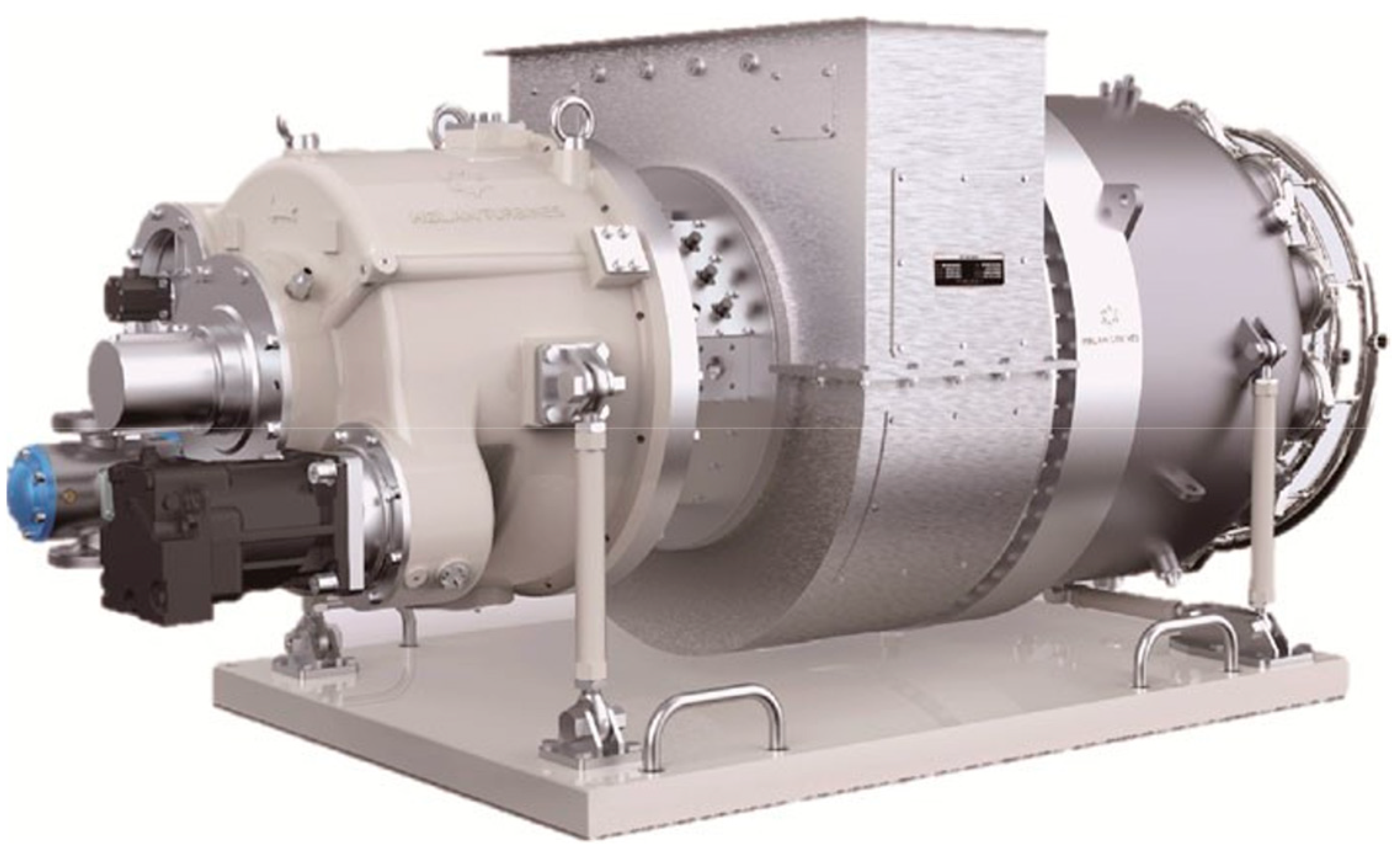
In response to the aforementioned issues, this study combines a fatigue damage assessment model considering temperature fluctuations with an online cycle counting method that takes into account temperature fluctuations during the cyclic process. A novel online fatigue damage assessment method is proposed to provide more accurate damage assessment of key components of gas turbines operating at high temperatures. This study selected 220 typical transient points from the experimental data of a micro gas turbine operating under a “cold start-full load-shutdown” cycle, which lasted for 5855 s. The corresponding temperature and stress distributions on the turbine vanes were calculated using CFD and FEA. The finite element calculation results were then utilized to train a surrogate model to traverse the entire temperature and stress variation process of the turbine vanes during the working cycle, which enabled fatigue damage assessment. It should be noted that the approach proposed in this paper is stress-based, and an elastic model should be employed during the finite element calculation. The structure of the micro gas turbine described in this study is illustrated in Figure 1, and the corresponding parameters are presented in

Table 1. Micro gas turbine parameters.

Parameter	Value
Power generation/MW	2
Power generation efficiency/%	25.7
Pressure ratio	7.5
Exhaust flow rate/(Kg/s)	10.1
Turbine inlet temperature/K	1223
Exhaust temperature/K	803

. The results indicate that the fatigue damage assessed using the method proposed in this study is D_f = 4.37 × 10⁻⁵. In comparison, the damage assessment based on the equivalent operating hours recommended by the OEM yields a value of D_OEM = 5.08 × 10⁻⁵. This method has the advantage of accurately and dynamically displaying the process of damage evolution, providing a visual representation of the structural integrity of the components.

The remaining sections of this paper are organized as follows: Section 2 presents an online cycle counting method that takes into account the cyclic characteristic temperature and the duration of cyclic loading. This algorithm is utilized for real-time processing of load information. Section 3 provides a fatigue damage assessment model for different deformation mechanisms and explains how to incorporate the influence of temperature fluctuations on fatigue damage. In Section 4, the proposed method in this paper is validated and the results are analyzed using experimental data from a micro gas turbine. Lastly, Section 5 summarizes the paper and provides an overview of the applicable scenarios, research limitations, and future research directions for this method.

2. Online Cycle Counting Method Considering the Characteristic Temperature of the Cycle

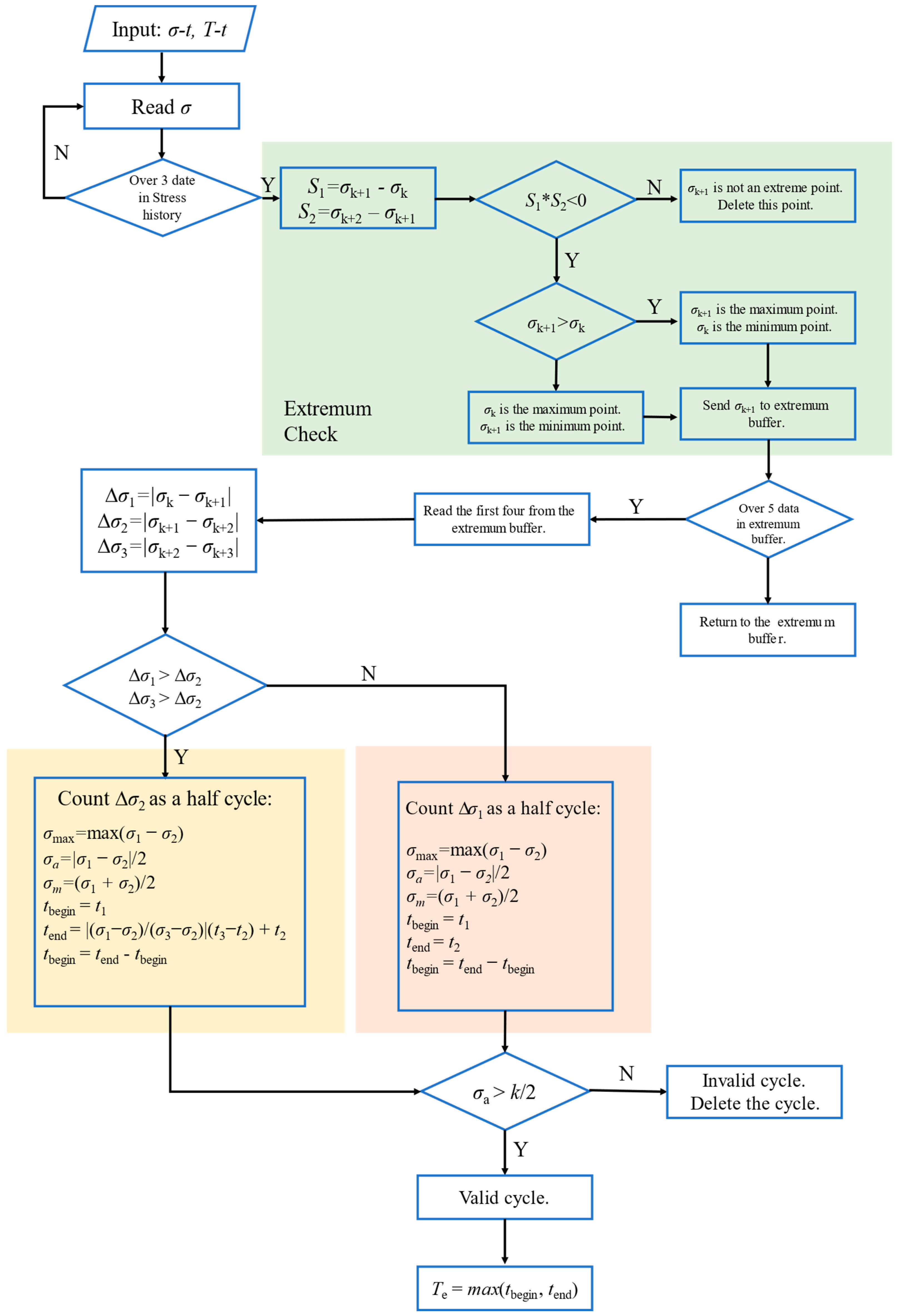
Based on the four-point online rainflow counting method, this paper proposes an improved online cycle counting method that considers temperature fluctuations during the cyclic process. The overall procedure is illustrated in Figure 2 and can be divided into four main parts: stress extremum identifying, cycle counting and cycle duration determining, invalid cycle eliminating, and characteristic temperature matching. These four parts will be described in detail in the following sections. It should be noted that the input of this algorithm is the stress-time and temperature-time information of the components during the operation of the gas turbine, which can be obtained through methods such as surrogate modeling, response surface methodology, and Kriging simulation [14,15,16].

Regarding the stress-time information, most of the existing fatigue damage assessment models calculate the Mises stress based on the fourth strength criterion and then perform strength calculations. The calculation formula is as follows:

$${\mathsf{\sigma }}_{\mathrm{e}}=\sqrt{\frac{1}{2}[{\left({\mathsf{\sigma }}_{\mathrm{x}} - {\mathsf{\sigma }}_{\mathrm{y}}\right)}^2+{\left({\mathsf{\sigma }}_{\mathrm{y}}- {\mathsf{\sigma }}_{\mathrm{z}}\right)}^2+{\left({\mathsf{\sigma }}_{\mathrm{z}}- {\mathsf{\sigma }}_{\mathrm{x}}\right)}^2+6({\mathsf{\tau }}_{\mathrm{xy}}^2+{\mathsf{\tau }}_{\mathrm{yz}}^2+{\mathsf{\tau }}_{\mathrm{zx}}^2\left)\right]}$$

(1)

where σ_x, σ_y, σ_z represents the normal stress on the X, Y, and Z planes, respectively, τ_xy represents the shear stress along the Y-axis on the X-plane, τ_yz represents the shear stress along the Z-axis on the Y-plane, τ_zx represents the shear stress along the X-axis on the Z-plane.

As can be seen from Equation (1), the Mises stress must be a positive value, representing the magnitude of the stress experienced by the component. It cannot determine the direction of the stress, thus unable to identify whether the component is under tension or compression. For certain components that experience both tensile and compressive stresses throughout the entire operating cycle, it is crucial to consider the direction of the stress. Failure to account for the stress direction may lead to significant errors in determining the stress range Δσ. To address this issue, the static hydrostatic pressure σ_h is introduced, and its calculation formula is as follows:

$${\mathsf{\sigma }}_{\mathrm{h}}=\frac{1}{3}({\mathsf{\sigma }}_{\mathrm{x}}+{\mathsf{\sigma }}_{\mathrm{y}}+{\mathsf{\sigma }}_{\mathrm{z}})$$

(2)

When σ_h > 0, σ_e is in the positive direction, indicating a tensile stress. When σ_h < 0, σ_e is in the opposite direction, indicating a compressive stress [17]. The verification component used in this paper is the turbine vanes, which are mainly subjected to thermal stresses caused by temperature variations. Throughout the entire operating cycle, the stress is predominantly compressive. Therefore, the algorithm in this study does not include a stress direction identification module. Stress is a tensor, so the range of stress should be as follows:

$$\mathsf{\Delta }{\mathsf{\sigma }}_{\mathrm{e}}=\frac{1}{\sqrt{2}}\sqrt{[{\left(\mathsf{\Delta }{\mathsf{\sigma }}_{\mathrm{x}} - \mathsf{\Delta }{\mathsf{\sigma }}_{\mathrm{y}}\right)}^2+{\left(\mathsf{\Delta }{\mathsf{\sigma }}_{\mathrm{y}} - \mathsf{\Delta }{\mathsf{\sigma }}_{\mathrm{z}}\right)}^2+{\left(\mathsf{\Delta }{\mathsf{\sigma }}_{\mathrm{z}} - \mathsf{\Delta }{\mathsf{\sigma }}_{\mathrm{x}}\right)}^2+6(\mathsf{\Delta }{\mathsf{\tau }}_{\mathrm{xy}}^2+\mathsf{\Delta }{\mathsf{\tau }}_{\mathrm{yz}}^2+\mathsf{\Delta }{\mathsf{\tau }}_{\mathrm{zx}}^2\left)\right]}$$

(3)

However, in this study, for two consecutive stresses σ₁ and σ₂, the stress range Δσ is directly calculated as Δσ = |σ₁ − σ₂| without considering the stress direction.

2.1. Stress Extremum Identifying

Previous research has shown that identifying the maximum and minimum values within a cycle is crucial for fatigue damage assessment, while any intermediate data points that are irrelevant to fatigue assessment can be eliminated. Stress extremum identifying aims to retain only the data points where the direction/slope reverses, requiring three consecutive data points. Let’s assume the stress values of these three consecutive data points are σ₁, σ₂ and σ₃.

If (σ₁ − σ₂) ∗ (σ₂ − σ₃) < 0, then σ₂ is considered an extremum point. If σ₂ > σ₁, then σ₂ is a local maximum point. If σ₂ < σ₁, then σ₂ is a local minimum point. In this case, σ₂ is stored in the stress extremum buffer, and the process continues to read new data points for new identification.

If (σ₁ − σ₂) ∗ (σ₂ − σ₃) > 0, then σ₂ is not an extremum point. In this case, σ₂ is eliminated, and the process continues to read new data points for new identification.

2.2. Cycle Counting and Cycle Duration Determining

As mentioned above, the cycle counting method used in this study is an improvement based on the concept of the four-point online rainflow counting. To ensure that the points read during each cycle counting are extreme points, the stress extremum buffer should store a minimum of five extremum. This allows for the determination of whether the fourth value is an extreme point based on the fifth value. Let’s assume that the stress values of the four consecutive extreme points read from the stress extremum buffer are σ₁, σ₂, σ₃ and σ₄. We define Δσ₁ = |σ₁ − σ₂|, Δσ₂ = |σ₂ − σ₃| and Δσ₃ = |σ₃ − σ₄|.

If Δσ₂ < Δσ₁ and Δσ₂ < Δσ₃, Δσ₂ is considered a full cycle. In this case, the maximum stress of the cycle is σ_max = max(σ₂, σ₃), the stress amplitude is σ_a = |σ₂ − σ₃|/2, the mean stress is σ_m = (σ₂ + σ₃)/2, and the cycle counting is 1. The points σ₂ and σ₃ are eliminated, while σ₁ and σ₄ are retained. The algorithm continues to read new points and re-identifies the cycles. 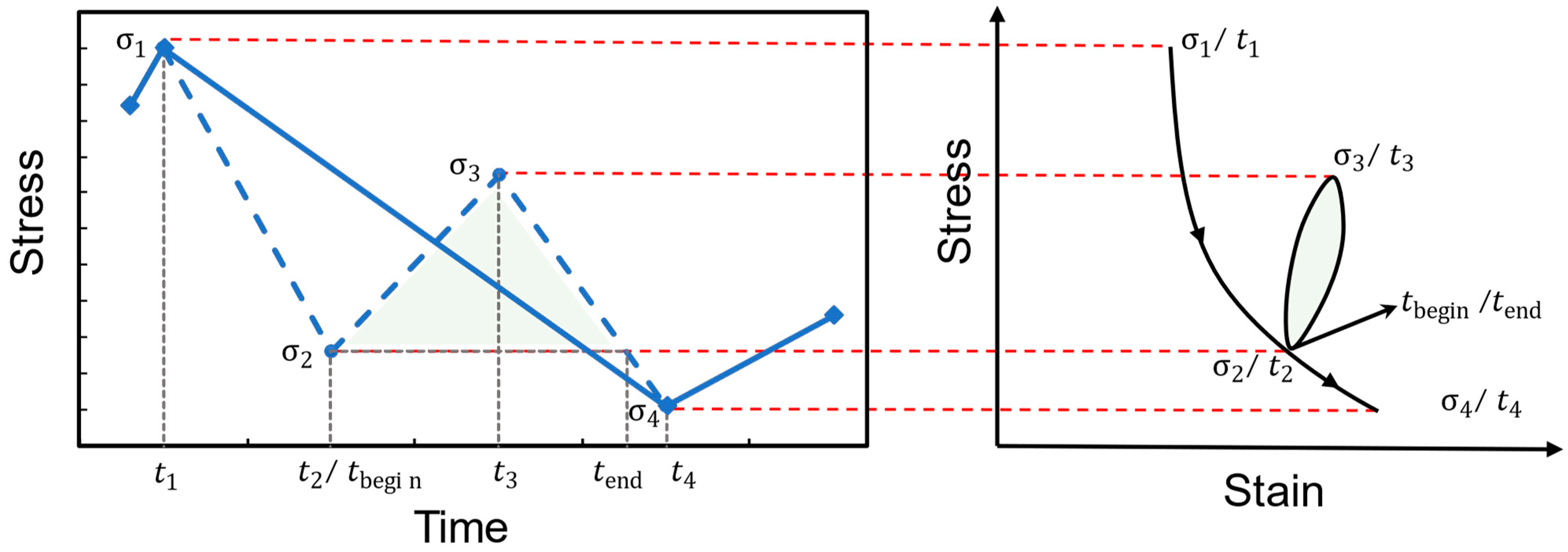In this study, we refer to the relationship between the load information and load duration in the case of a full cycle as proposed by GopiReddy [18] for online assessment of creep damage based on rainflow counting. We introduce the concepts of cycle start time t_begin, cycle end time t_end and cycle duration t_hold for assessing the online fatigue damage in the case of a full cycle. Please refer to Figure 3 for a graphical representation. The calculation formulas are as follows:

$${\mathit{t}}_{\mathrm{begin}}={\mathit{t}}_2$$

(4)

$${\mathit{t}}_{\mathrm{end}}=|\frac{{\mathsf{\sigma }}_2-{\mathsf{\sigma }}_3}{{\mathsf{\sigma }}_4-{\mathsf{\sigma }}_3}\left({\mathit{t}}_4-{\mathit{t}}_3\right)| +{ \mathit{t}}_3$$

(5)

$${\mathit{t}}_{\mathrm{hold}}={ \mathit{t}}_{\mathrm{end}}-{ \mathit{t}}_{\mathrm{begin}}$$

(6)

where t₁, t₂, t₃ and t₄ represents the time corresponding to σ₁, σ₂, σ₃ and σ₄, respectively.

If Δσ₁ > Δσ₂ > Δσ₃, Δσ₂ > Δσ₁ > Δσ₃, Δσ₂ > Δσ₃ > Δσ₁ or Δσ₃ > Δσ₂ > Δσ₁, Δσ₁ is considered a half-cycle. In this case, the maximum stress of the cycle is σ_max = max(σ₁, σ₂), the stress amplitude is σ_a = (|σ₁ − σ₂|)/2, the mean stress is σ_m = (σ₁ + σ₂)/2, and the cycle counting is 0.5. The point σ₁ is eliminated, while σ₂, σ₃, and σ₄ are retained. The algorithm continues to read new points and re-identifies the cycles. Referring to the full-cycle time matching method, the half-cycle time information are as follows:

$$t_{\mathrm{b}\mathrm{e}\mathrm{g}\mathrm{i}\mathrm{n}}=t_1$$

(7)

$${\mathit{t}}_{\mathrm{end}}={\mathit{t}}_2$$

(8)

$${\mathit{t}}_{\mathrm{hold}}={\mathit{t}}_{\mathrm{end}} - {\mathit{t}}_{\mathrm{begin}}$$

(9)

2.3. Invalid Cycle Eliminating

The purpose of invalid cycle elimination is to eliminate insignificant fluctuations in damage accumulation. The determination of invalid cycles requires a threshold value k, which is influenced by various variables such as operating speed, output power, and gas turbine structure. The value of k may vary under different conditions. The threshold value k used in this study is specific to a micro gas turbine of a certain model. It should be noted that the determination of the threshold value k does not affect the proposed method in this study.

For the identified cycles, if σ_a > k/2, it is considered a valid cycle and retained. If σ_a < k/2, it is considered an invalid cycle and removed.

2.4. Characteristic Temperature Matching

The characteristic temperature refers to the temperature that best represents the identified cycle’s temperature history. The specific selection method should consider the relationship between temperature and material properties. In this study, we have provided several commonly used engineering methods for selecting the characteristic temperature, as described below:

$${\mathit{T}}_{\mathrm{e}}=\mathrm{maxT} ({\mathit{t}}_{\mathrm{begin}},{\mathit{t}}_{\mathrm{end}})$$

(10)

$${\mathit{T}}_{\mathrm{e}}=\mathit{W}\mathrm{maxT} ({\mathit{t}}_{\mathrm{begin}},{\mathit{t}}_{\mathrm{end}})+ (1-\mathit{W})\mathrm{minT} ({\mathit{t}}_{\mathrm{begin}},{\mathit{t}}_{\mathrm{end}})$$

(11)

$${\mathit{T}}_{\mathrm{e}}=\mathit{T}\left({\mathsf{\sigma }}_{\max }\right)$$

(12)

where T_e represents the characteristic temperature of the identified cycle. W represents the weight factor, typically set to 0.75. $\mathit{T}\left({\mathsf{\sigma }}_{\max }\right)$ represents the temperature corresponding to the maximum stress point in the cycle.

2.5. Example Analysis

To better illustrate how the proposed algorithm works, it was applied to a dataset containing 21 pairs of stress-temperature-time samples. The distribution of the data is shown in Figure 4. For the convenience of the example, it is assumed that the sampling frequency is 1 s and the threshold value for invalid cycle determination k is 10 Mpa.

When accumulating three data points, we can perform the identification of extremum points. At this stage, we have (111 − 106) × (106 − 87) > 0, indicating that 106 MPa is a non-extremum point and should be removed. We reading new data points, and now we have (111 − 87) × (87 − 108) < 0 and 87 < 111, indicating that 87 MPa is a local minimum and should be stored in the extremum value buffer. We continue reading new data points, and now we have (87 − 108) × (108 − 90) < 0 and 108 > 87, indicating that 108 MPa is a local maximum and should be stored in the extremum value buffer. We repeat this process to continue the identification of extremum points.

When the extremum value buffer already contains four extremum points and we read the fifth data point, the cycle counting begins. At this time, the extremum value buffer contains [111, 87, 108, 90], and the new data point is σ₅ = 112 MPa. We can determine that σ₄ is a local minimum. In this case, Δσ₁ = |111 − 87| = 24 MPa, Δσ₂ = |87 − 108| = 21 MPa, and Δσ₃ = |108 − 90| = 18 MPa. Since Δσ₁ > Δσ₂ > Δσ₃, we can conclude that Δσ₁ constitutes a half cycle. For this cycle, σ_max = 111 MPa, σ_a = (|111 − 87|)/2 = 12 MPa, σ_m = (111 + 87)/2 = 99 MPa, cycle counting is 0.5, t_begin = 1 s, t_end = 3 s, t_hold = 3 − 1 = 2 s, and the cycle’s characteristic temperature is T_e = maxT(t_begin, t_end) = 442.04 °C. Since σ_a = 12 > k/2, this cycle is considered valid, and σ₁ can be removed.

Continuing with the new data point, the extremum value buffer now becomes [87, 108, 90, 112]. With the new data point σ₅ = 108 MPa, we can determine that σ₄ is a local maximum. In this case, Δσ₁ = |87 − 108| = 21 MPa, Δσ₂ = |108-90| = 18 MPa, and Δσ₃ = |90 − 112| = 22 MPa. Since Δσ₂ < Δσ₁ and Δσ₂ < Δσ₃, we can conclude that Δσ₂ constitutes a full cycle. For this cycle, σ_max = 108 MPa, σ_a = (|108 − 90|)/2 = 9 MPa, σ_m = (108 + 90)/2 = 99 MPa, cycle counting is 1, t_begin = 4 s, t_end = (108 − 90)/(112 − 90) × (6 − 5) + 5 = 5 s, t_hold = 5.82 − 3.14 = 2.68 s, and T_e = maxT(t_begin, t_end) = 451.44 °C. Since σ_a = 9 > k/2, this cycle is considered valid, and σ₂, σ₃ can be removed.

Continuing with the new data points, the extremum value buffer becomes [87, 112, 108, 87]. Based on the condition (112 − 108) × (108 − 87) > 0, we can determine that σ₃ is a non-extremum point and should be removed. Moving on to the new data points, the extremum value buffer becomes [87, 112, 87, 82]. Using the condition, (112 − 87) × (87 − 82) > 0, we can conclude that σ₃ is a non-extremum point and should be removed.

Continuing with the new data points, the extremum value buffer becomes [87, 112, 82, 90]. Based on the new data point σ₅ = 85 Mpa, we can determine that σ₄ is a local maximum. In this case, Δσ₁ = |87 − 112| = 25 Mpa, Δσ₂ = |112 − 82| = 30 Mpa, Δσ₃ = |82 − 90| = 8 Mpa. Since Δσ₂ > Δσ₁ > Δσ₃, we can conclude that Δσ₁ constitutes a half cycle. For this half cycle, σ_max = 112 Mpa, σ_a = (|87 − 112|)/2 = 12.5 Mpa, σ_m = (112 + 87)/2 = 99.5 Mpa, cycle counting is 0.5, t_begin = 3 s, t_end = 6 s, t_hold = 6 − 3 = 3 s, and T_e = maxT(t_begin, t_end) = 482.76 °C. Since σ_a = 12.5 > k/2, this cycle is considered valid, and σ₁ should be removed. The subsequent calculations can be found in

Table 2. Rainflow cycle counting process of proposed method.

Time (s)	Stress (Mpa)	[Δσ1 Δσ2 Δσ3] (Mpa)	FC/HC	σa (Mpa)	tbegin (s)	tend (s)	Te (°C)
[1 2 3 4 5]	[111 106 87 108 90]
[1 3 4 5 6]	[111 87 108 90 112]	[24 21 18]	HC	12	1	3	442.04
[3 4 5 6 7]	[87 108 90 112 108]	[21 18 22]	FC	9	4	5.82	451.44
[3 6 7 8 9]	[87 112 108 87 82]
[3 6 8 9 10]	[87 112 87 82 90]
[3 6 9 10 11]	[87 112 82 90 85]	[25 30 8]	HC	12.5	3	6	482.76
[6 9 10 11 12]	[112 82 90 85 89]	[30 8 5]	HC	15	6	9	489.01
[9 10 11 12 13]	[82 90 85 89 115]
[9 10 11 13 14]	[82 90 85 115 106]	[8 5 30]		2.5
[9 13 14 15 16]	[82 115 106 102 116]
[9 13 15 16 17]	[82 115 102 116 85]	[33 13 14]	FC	6.5	13	15.92	474.12
[9 16 17 18 19]	[82 116 85 118 86]	[34 31 33]	FC	15.5	16	17.93	462.48
[9 18 19 20 21]	[82 118 86 102 106]
[9 18 19 21]	[82 118 86 106]	[36 32 20]	HC	18	9	18	486.05

.

3. Fatigue Damage Assessment

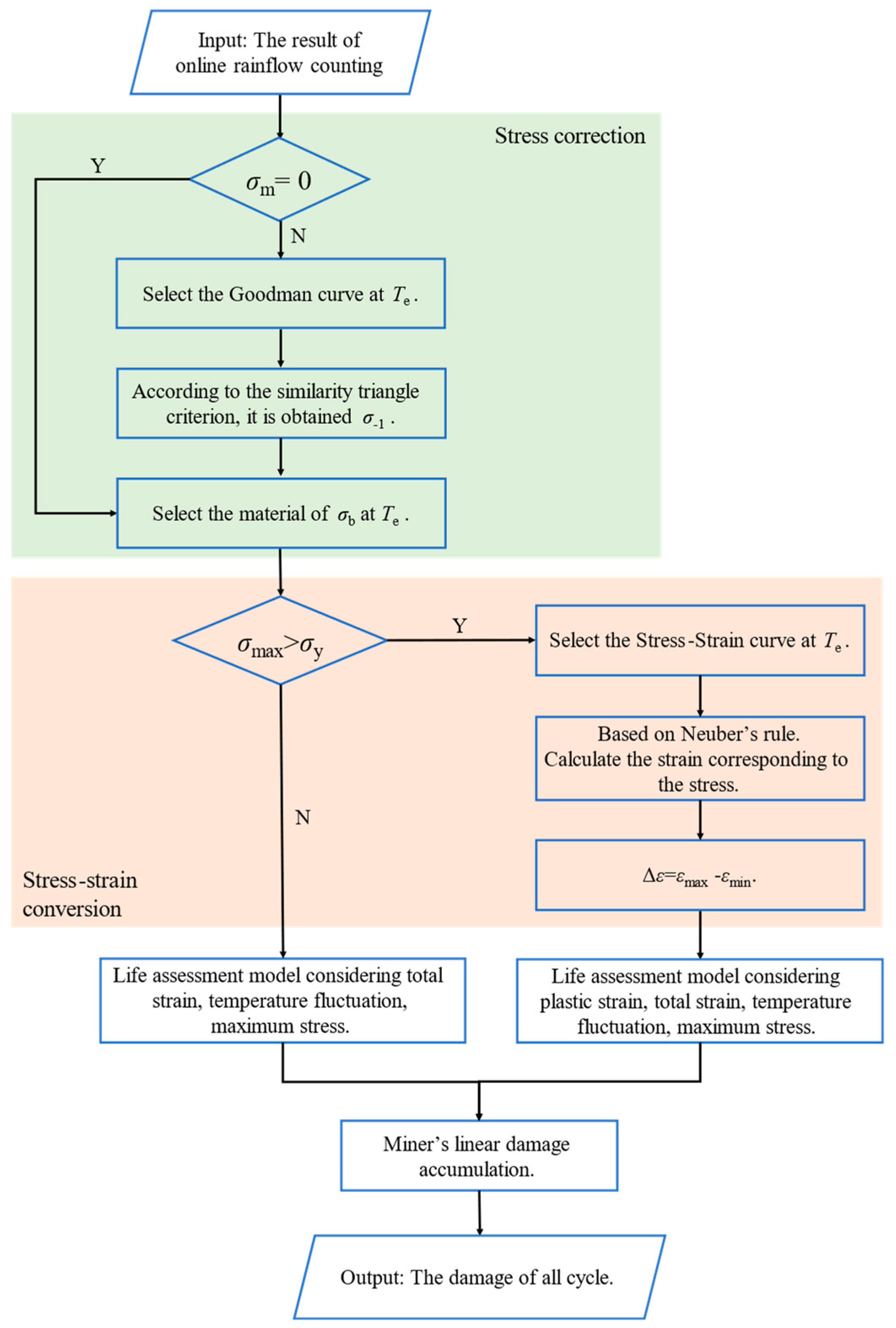
As mentioned above, based on the cycle counting method considering the characteristic temperature, we have identified valid full cycles and half cycles, and determined the characteristic temperature of the identified cycles. After further processing the stress and temperature information of the identified cycles, we can apply the fatigue damage model developed by our research team, which considers the influence of temperature, to assess the life of components. The overall process is illustrated in Figure 5. Here, we provide a brief introduction to the model, which can be divided into three parts: stress correction, stress-strain conversion, and fatigue damage assessment model considering temperature fluctuations.

3.1. Stress Correction

In practical applications, components are often subjected to irregularly random loads, while testing conditions of laboratories often involve symmetric cyclic loads or pulse loads. In order to better match the actual conditions with the experimental conditions, we need to correct the actual loads using the Goodman curve.

Assuming that the mean stress and stress amplitude of any cycle are denoted as σ_m and σ_a, and the maximum and minimum stresses of the cycle are denoted as σ_max and σ_min, the calculation formulas for σ_m and σ_a are as follows:

$${\mathsf{\sigma }}_{\mathrm{m}}=\frac{1}{2}\left({\mathsf{\sigma }}_{\max }+{\mathsf{\sigma }}_{\min }\right)$$

(13)

$${\mathsf{\sigma }}_{\mathrm{a}}=\frac{1}{2}({\mathsf{\sigma }}_{\max } - {\mathsf{\sigma }}_{\min })$$

(14)

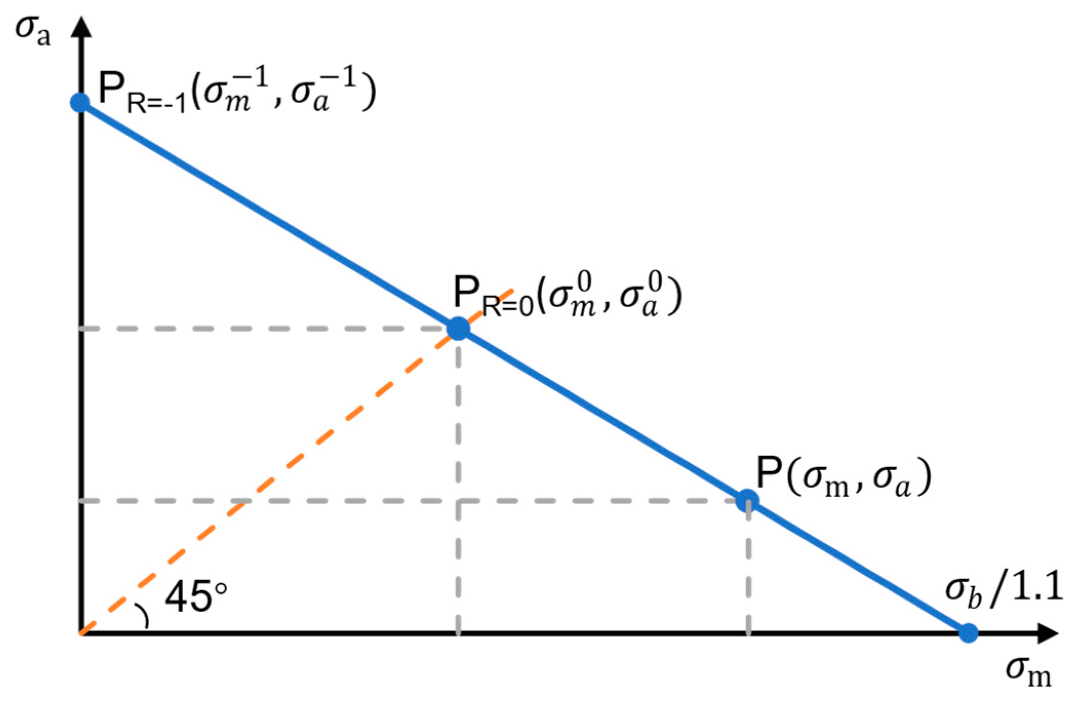
The Equivalent Life Goodman Diagram is illustrated in Figure 6, which depicts the relationship between the fatigue point P and its equivalent life fatigue points P_(R=0) and P_(R=−1). When σ_m = σ_a, the corresponding equivalent life pulsating cyclic fatigue point to P is P_(R=0) (σ_m⁰, σ_a⁰). When σ_m = 0, the corresponding equivalent life symmetrical cyclic fatigue point to P is P_(R=−1) (σ_m⁻¹, σ_a⁻¹). By applying the principle of similar triangles, we can obtain the corrected stress information for point P under different scenarios [19]. It should be noted that the equivalent life curves of materials vary with different temperatures, and σ_b represents the fatigue limit of the material at a specific temperature. In this study, the fatigue damage assessment model considers the influence of mean stress on fatigue damage, so there is no need to correct the stress of the identified cycle. In the opposite case, stress correction is required.

3.2. Stress-Strain Conversion

Plastic strain generated during material plastic deformation is a decisive factor affecting fatigue damage. The above method only counts stress throughout the entire process and does not provide information about the deformation of the component under the stress-temperature levels of the identified cycle. By comparing σ_max of the identified cycle with the yield strength σ_y of the material used in the component at T_e of the identified cycle, if the former is greater than the latter, it is considered that plastic deformation has occurred in the component, and its plastic strain can be calculated. In this study, stress and strain for a process of a cycle are considered as scalars, without taking into account their direction. Furthermore, when the component undergoes plastic deformation, the Mises stress obtained based on the elastic theory is higher than the actual stress experienced by the component, as illustrated in Figure 7. In order to rectify this, we can apply the Neuber’s rule.

The Neuber’s rule [20] describes the relationship between the local notch response and the applied elastic load as follows:

$$\mathsf{\epsilon }\mathsf{\sigma } =\frac{{\left({\mathit{K}}_{\mathrm{t}}\mathit{S}\right)}^2}{\mathit{E}}$$

(15)

where K_t represents the theoretical stress concentration factor, S is the elastic stress, E is the elastic modulus.

For a process of a cycle, the local notch response follows the stress-strain curve, which is commonly represented by the Ramberg-Osgood equation defined as follows:

$$\mathsf{\epsilon }=\frac{\mathsf{\sigma }}{\mathit{E}}+{(\frac{\mathsf{\sigma }}{\mathit{K}})}^{\frac{1}{{\mathit{n}}^{\prime }}}$$

(16)

where K denotes the strain-hardening coefficient, and n′ is the strain hardening exponent.

Here, unlike the traditional offline conversion method, the stress range and strain range cannot be roughly replaced by the stress amplitude and strain amplitude. The conversion relationship between the two as follows:

$$∆{\mathsf{\epsilon }}_{\mathrm{a}}=\frac{{\mathsf{\sigma }}_{\max } - {\mathsf{\sigma }}_{\min }}{\mathit{E}}+{ 2\left[\right(\frac{{\mathsf{\sigma }}_{\max }}{\mathit{K}})}^{\frac{1}{{\mathit{n}}^{\prime }}}-{\left(\frac{{\mathsf{\sigma }}_{\min }}{\mathit{K}}\right)}^{\frac{1}{{\mathit{n}}^{\prime }}}]$$

(17)

where Δε_a is the total strain range.

The stress-strain curve varies with temperature. To ensure the accuracy of the conversion results, the characteristic temperature of the identified cycle is used as the reference temperature for the selection of the stress-strain curve at conversion.

3.3. Fatigue Damage Assessment Model Taking into Account Temperature Fluctuations

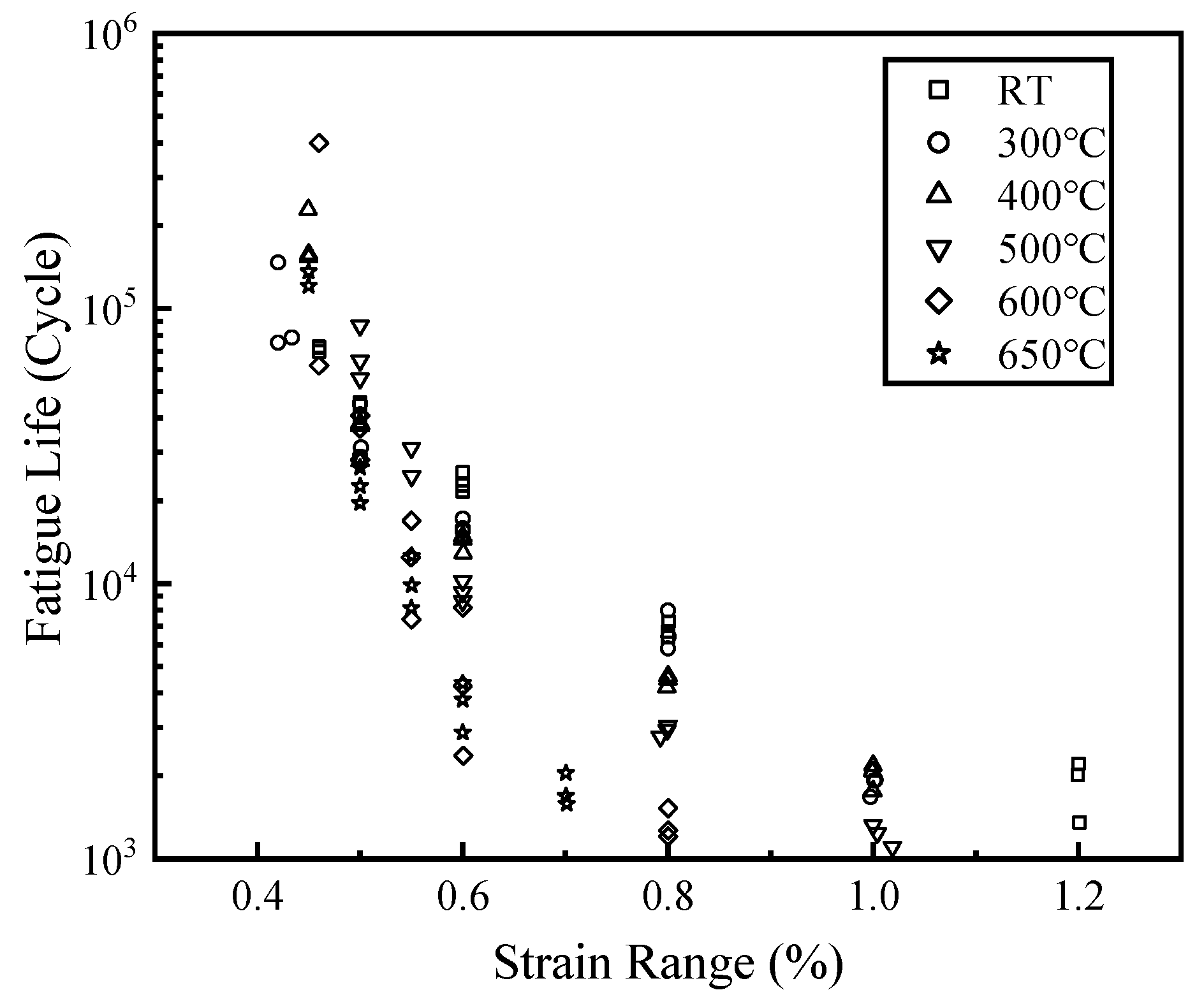
The fatigue damage assessment model considering temperature fluctuations used in this study is based on low-cycle fatigue tests conducted on a nickel-based high-temperature alloy at different temperatures. The low-cycle fatigue tests were performed on an MTS hydraulic servo testing machine at room temperature (RT), 300 °C, 400 °C, 500 °C, 600 °C, and 650 °C. The tests were conducted using axial displacement control and a total strain ratio R_ε=−1. The cycle’s waveform used was triangular, and the strain amplitude was controlled within the range of 0.4% to 1.2% strain level. The tests were continued until the specimen fractured. The relationship between the strain range and fatigue damage at each test temperature is shown in Figure 8.

When the component does not experience plastic deformation, this study adopts the SWT (Smith, Watson, and Topper) model [7] that takes into account the total strain range Δε_a, maximum stress σ_max, and temperature fluctuations as the assumed fatigue damage model. It is represented as follows:

$${\mathsf{\sigma }}_{\max }\mathsf{\Delta }{\mathsf{\epsilon }}_{\mathrm{a}}=\frac{{\left({\mathsf{\sigma }}_{\mathrm{f}}^{\prime }\right)}^2}{\mathit{E}}{\left(2{\mathit{N}}_{\mathrm{f}}\right)}^{2\mathrm{b}}+{\mathsf{\epsilon }}_{\mathrm{f}}^{\prime }{\mathsf{\sigma }}_{\mathrm{f}}^{\prime }{\left(2{\mathit{N}}_{\mathrm{f}}\right)}^{\mathrm{b}+\mathrm{c}}$$

(18)

where σ_f′ represents the fatigue strength coefficient, ε_f′ represents the fatigue ductility coefficient, b represents the fatigue strength exponent, and c represents the fatigue ductility exponent.

In the (18), σ_f′, E, b, ε_f′ and c are all functions of temperature. In this study, in order to consider the effect of temperature fluctuations on fatigue damage, the above parameters will be selected according to the characteristic temperature of the identified cycle.

The relationship between the yield stress of the nickel-based high-temperature alloy and temperature is illustrated in Figure 9.

When plastic deformation occurs in the component, this study will choose a method [21] that considers the plastic strain range Δε_pa, the total strain range Δε_a and the maximum stress σ_max as the fatigue damage assessment model. Besides, the new model introduces f(T) to describe the effect of temperature fluctuations on fatigue damage. The form of the temperature correction term in the new model and the validation of the accuracy of the model have been carried out in previous work and are represented as follows:

$$2{\mathit{N}}_{\mathrm{f}}=\mathrm{A}\mathsf{\Delta }{\mathsf{\epsilon }}_{\mathrm{pa}}^{{\mathit{n}}_1}\mathsf{\Delta }{\mathsf{\epsilon }}_{\mathrm{a}}^{{\mathit{n}}_2}{\mathsf{\sigma }}_{\max }^{{\mathit{n}}_3}{10}^{{\mathit{n}}_4{\mathit{T}}_{\mathrm{e}}}$$

(19)

where A, n₁, n₂, n₃ and n₄ are undetermined constants, Δε_pa represents the plastic strain range.

Finally, for a full cycle, the inverse of the fatigue damage is used as the fatigue damage for the cycle, while for a half cycle, only half of the inverse of the fatigue damage is used as the fatigue damage for the cycle. The total fatigue damage is calculated by linearly superimposing the fatigue damage for each cycle according to the Miner linear damage criterion, which is expressed as follows:

$${\mathit{D}}_{\mathrm{f}}=\sum \frac{\mathit{n}}{{\mathit{N}}_{\mathrm{f}}}$$

(20)

4. Application to Components and Results

In order to verify the aforementioned method, this study utilized experimental data from a micro gas turbine for the “cold start-full load-shutdown” sequence lasting 5855 s. A total of 220 representative transient points were selected for calculating the temperature field, and for conducting static analysis of the turbine vane model using the open-source finite element software CalculiX (Version 2.18). The static analysis employed an elastic finite element model, with the nickel-based high-temperature alloy shown in Figure 8 being used as the engineering material. Due to the significant time cost involved in the calculation, only 1/29 of the entire turbine vane was analyzed. The mesh structure of the microturbine vane is illustrated in Figure 10. 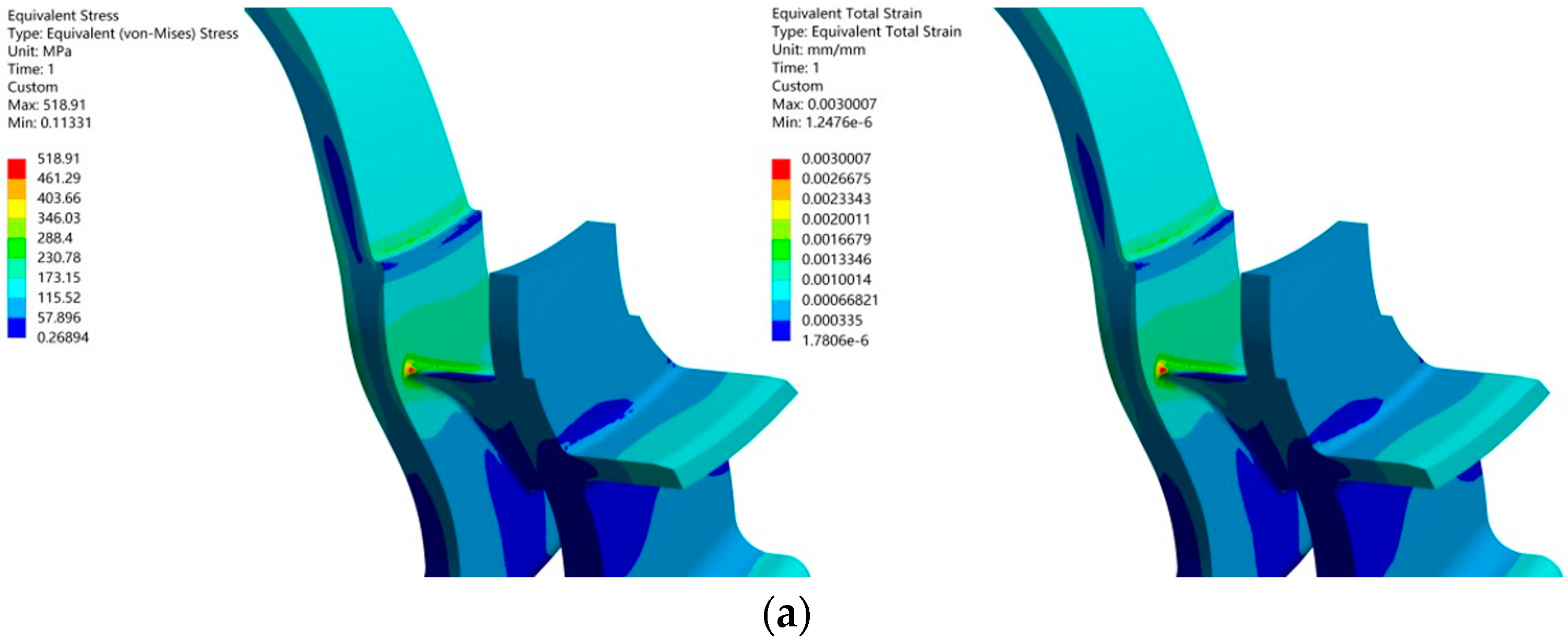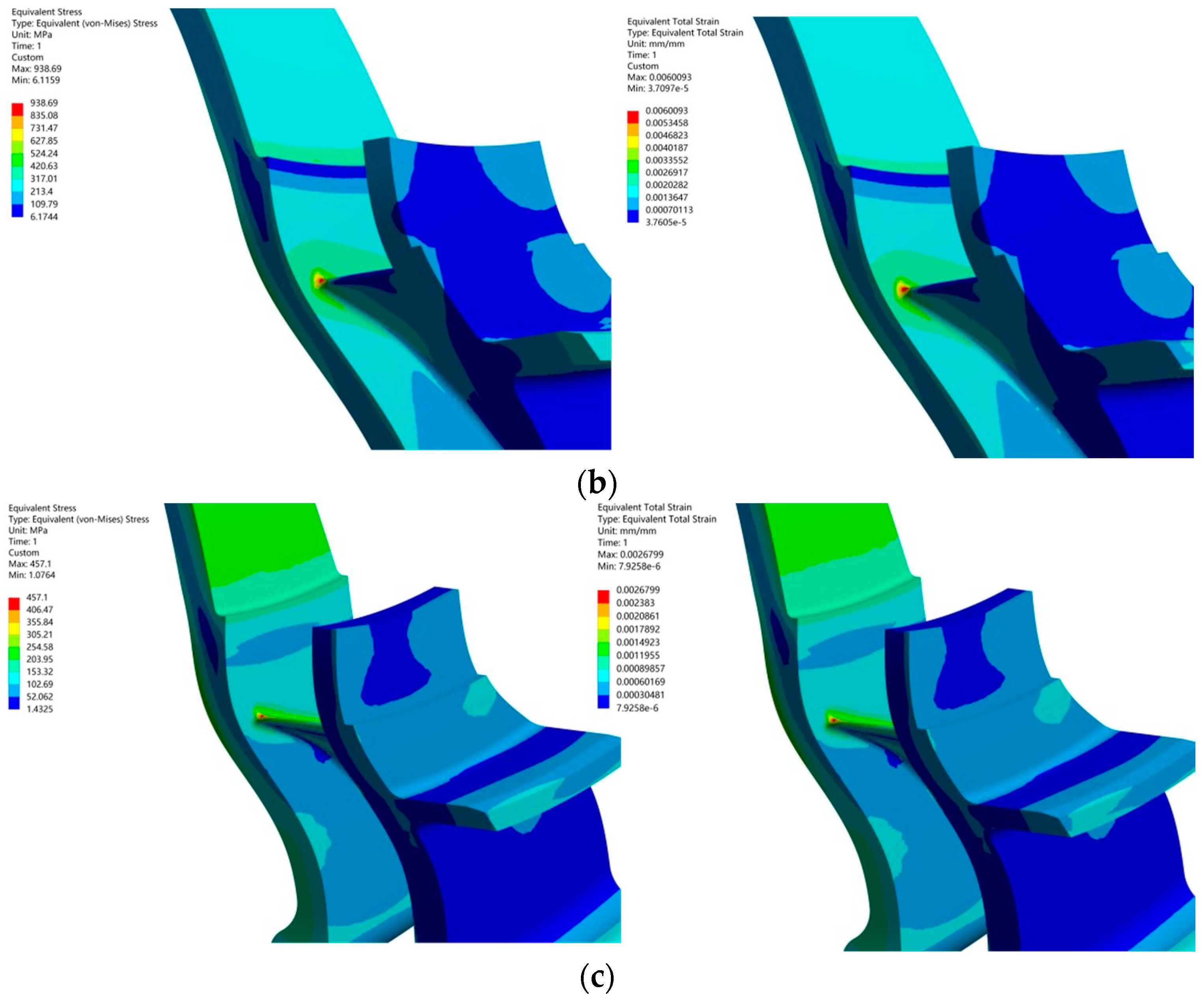Based on the simulation results, it can be concluded that the leading edge of the turbine vane is the most critical region, as illustrated in Figure 11. As mentioned above, the tensile and compressive nature of the critical region can be determined using Equation (2). The three-dimensional stress states of the critical region in “cold start-full load-shutdown” are illustrated in Figure 12. It should be noted that in this study, “shutdown” refers to the micro gas turbine not operating at an output power level. However, at this stage, the temperature of various components remains high. The residual stress resulting from this phenomenon has not been considered in this study.

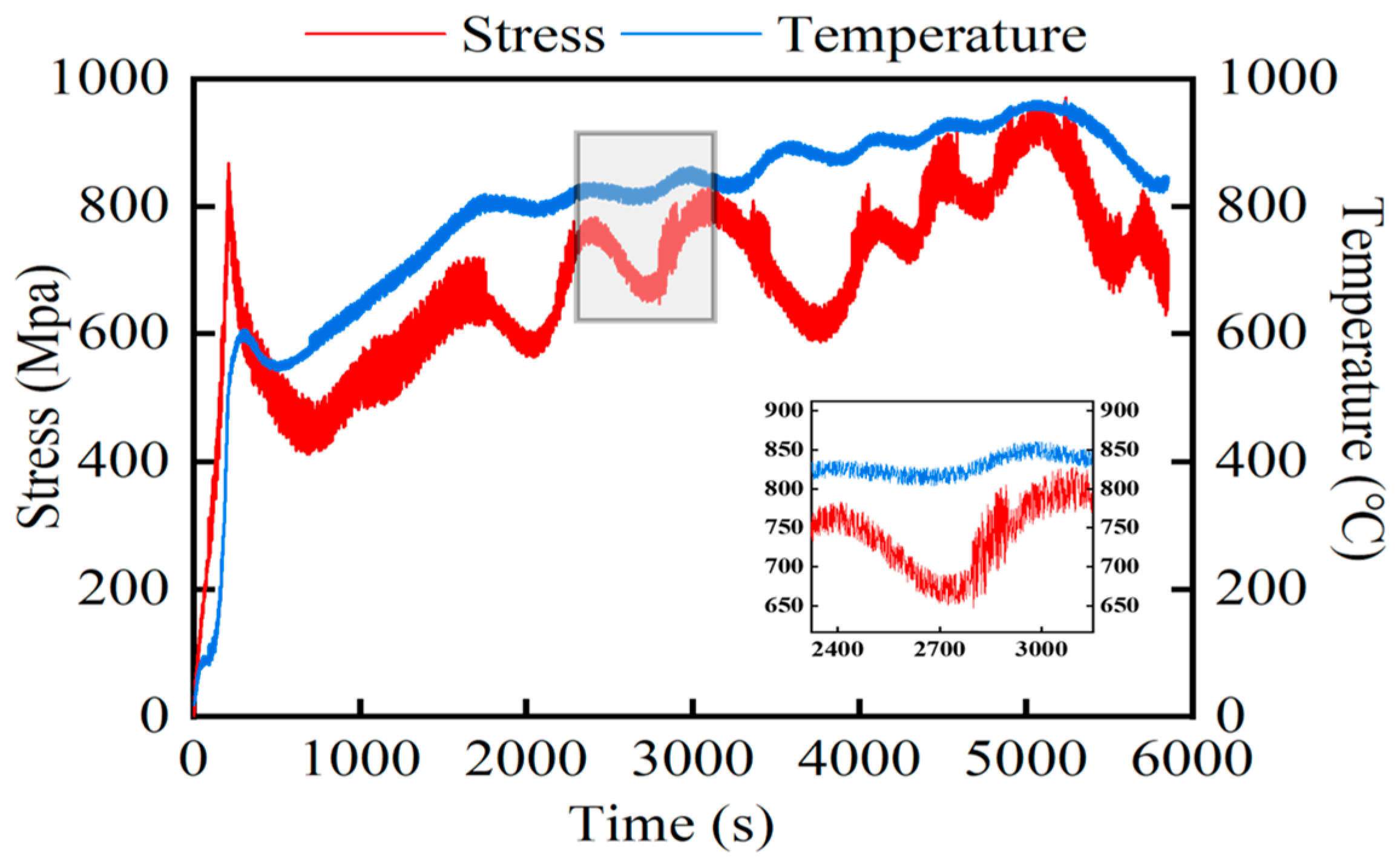
Throughout the entire process, the stress and temperature of the turbine vanes varied continuously, while the selected transient points could only reflect the stress and temperature information at the current moment. To obtain the stress and temperature information of the turbine vane throughout the entire operation, this study employed the damage surrogate model proposed by Boris Vasilyev et al. [22]. The model was trained using the power, rotational speed, fuel flow rate, and cross-sectional parameters of the gas turbine components at the selected 220 typical transient points as inputs and the stress and temperature information of critical points obtained from finite element calculations as outputs. 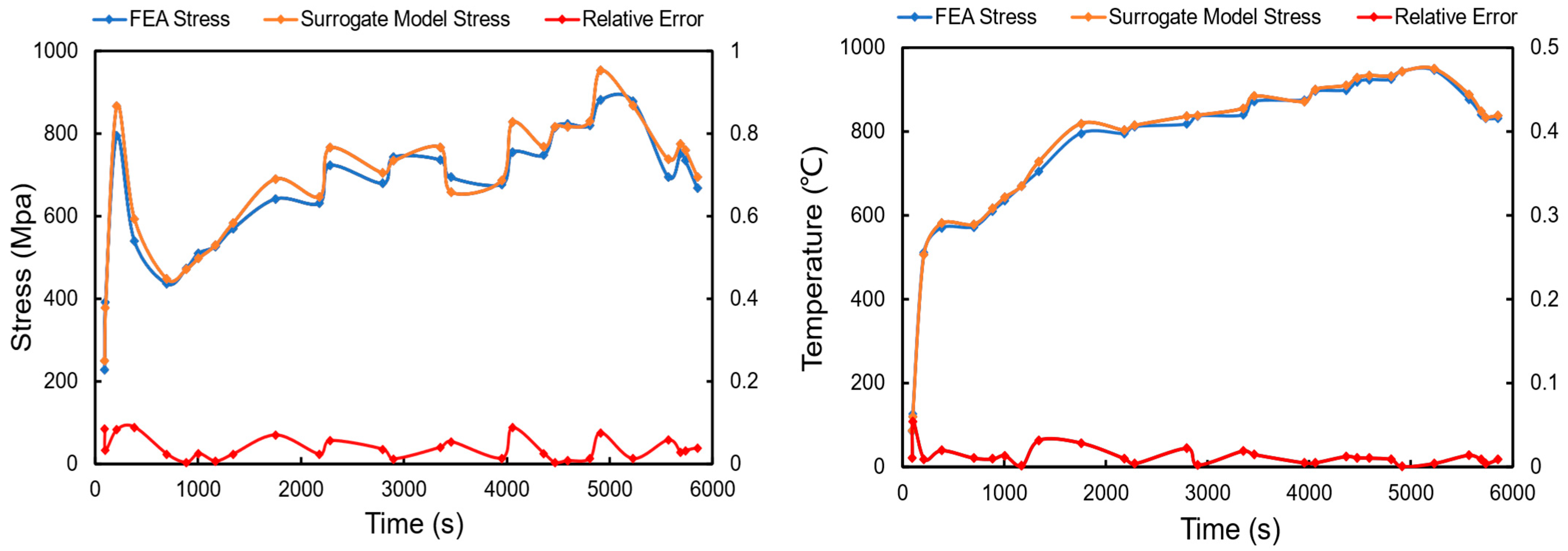By utilizing the surrogate model, the loading conditions of critical points in the entire “cold start-full load-shutdown” process of the turbine vanes were determined, as shown in Figure 13. To verify the accuracy of the surrogate model, 28 transient points were randomly selected from Figure 13, and the loading conditions of critical points at those moments were simulated using finite element analysis. The results, as shown in Figure 14, indicated an error within 10%, validating the reasonableness of the surrogate model’s generated data.

Based on factors such as the overall layout of the gas turbine, component material selection, and operating conditions, a threshold value of $k$ = 30 MPa was established to determine an invalid cycle. The data from Figure 13 were sampled every second, and the algorithm was executed to identify the valid cycles. The damage caused to the turbine vanes throughout the process was determined to be D_f = 4.37 × 10⁻⁵. The recommended overhaul period for this gas turbine according to its maintenance manual is 32,000 h, which corresponds to a damage value of D_OEM = 5.08 × 10⁻⁵ for this cycle.

Since the small gas turbine used in this study did not undergo long-term operation and only underwent short-term load variation and start-stop tests, fatigue was the primary damage mechanism for its components. Consequently, the influence of mechanisms such as creep, erosive wear, and oxidation corrosion was not considered in the damage assessment. As a result, the calculated results of the new method were lower than the values recommended by the OEM. Additionally, this study selected the maximum temperature within the cycle duration as the characteristic temperature for cycle counting and considered the influence of half cycles. When selecting the life assessment model, we considered the impact of temperature fluctuations on fatigue damage. These factors made the final damage assessment results more conservative than traditional methods, resulting in the new method’s calculated results being close to the recommended values by the OEM, which considers multiple damage mechanisms. In summary, the calculated results of the new method are within a reasonable range, confirming its accuracy.

5. Conclusions

This study proposes a new online real-time fatigue damage assessment method. The proposed method combines cycle counting with cycle duration and selects a characteristic temperature that can better reflect the temperature characteristics during the cycle process. The new characteristic temperature is then used in subsequent stress-strain conversion and life model parameter fitting, improving the accuracy of fatigue damage assessment.

This study presents a real-time online fatigue damage assessment of the turbine vanes during the cold-start process of a micro gas turbine. The obtained damage assessment results closely align with the recommended damage values by the OEM, thereby confirming the feasibility and practicality of the proposed methodology. By providing real-time output of the damage results, it enables an accurate reflection of the relationship between damage increment and current load. This in turn offers a reliable reference for condition-based maintenance of gas turbines. Additionally, it is worth noting that:

• This method is not limited to the fatigue damage assessment of hot-end components of gas turbines. If time-varying temperature/stress information is obtained, the same concept can be applied to the online fatigue damage assessment of other equipment and components. However, it is important to note that the fatigue damage assessment models may vary under different circumstances.
• The surrogate model applied in this study for obtaining real-time temperature/stress information is specific to the cold-start process of the mentioned micro gas turbine. If the intention is to extend its applicability to other equipment and components, it would be necessary to construct a new surrogate model that can reflect temperature/stress information in real-time based on operational data.
• Based on the experimental data of the micro gas turbine, the relative error between the results obtained from finite element calculations and the output of the surrogate model is within 10%. The proposed online fatigue damage assessment method in this study closely aligns with the recommended values provided by the OEM. Increasing the amount of training data for the surrogate model and incorporating physical laws within the surrogate model can enhance its output accuracy. Conducting metallographic tests or accelerated life tests on turbine vanes can further validate the accuracy of the proposed method in this study.