Forecasting Day-Ahead Electricity Prices for the Italian Electricity Market Using a New Decomposition—Combination Technique

Abstract

Over the last 30 years, day-ahead electricity price forecasts have been critical to public and private decision-making. This importance has increased since the global wave of deregulation and liberalization in the energy sector at the end of the 1990s. Given these facts, this work presents a new decomposition–combination technique that employs several nonparametric regression methods and various time-series models to enhance the accuracy and efficiency of day-ahead electricity price forecasting. For this purpose, first, the time-series of the original electricity prices deals with the treatment of extreme values. Second, the filtered series of the electricity prices is decomposed into three new subseries, namely the long-term trend, a seasonal series, and a residual series, using two new proposed decomposition methods. Third, we forecast each subseries using different univariate and multivariate time-series models and all possible combinations. Finally, the individual forecasting models are combined directly to obtain the final one-day-ahead price forecast. The proposed decomposition–combination forecasting technique is applied to hourly spot electricity prices from the Italian electricity-market data from 1 January 2014 to 31 December 2019. Hence, four different accuracy mean errors—mean absolute error, mean squared absolute percent error, root mean squared error, and mean absolute percent error; a statistical test, the Diebold–Marino test; and graphical analysis—are determined to check the performance of the proposed decomposition–combination forecasting method. The experimental findings (mean errors, statistical test, and graphical analysis) show that the proposed forecasting method is effective and accurate in day-ahead electricity price forecasting. Additionally, our forecasting outcomes are comparable to those described in the literature and are regarded as standard benchmark models. Finally, the authors recommended that the proposed decomposition–combination forecasting technique in this research work be applied to other complicated energy market forecasting challenges.

1. Introduction

In today’s liberalized electricity market, price forecasting has become challenging for everyone involved. Accurate and efficient electricity price forecasts represent an advantage for market players (buyers and suppliers) and are crucial for risk management. In particular, the forecasting of electricity prices is vital for cash-flow analysis, investment budgeting, securities markets, regulatory formulation, and centralized resource planning. Therefore, electricity price modeling and forecasting could help in evaluating bilateral contracts. Moreover, an electricity price forecast is essential for manufacturing enterprises that must implement offers for the spot market at short notice: determine the guidelines of the medium-term contracts, and set out their long-term development plans. However, the behavior of the electricity price varies from that of other financial and commodity markets because it has unique characteristics connected to its physical attributes that can dramatically alter pricing. The primary difference is that electricity is a commodity that cannot be stored, so a slight change in output can result in large price swings in a matter of hours or minutes. For example, spot electricity prices exhibit long-term trends (linear or nonlinear), seasonality (daily, weekly, seasonal, and yearly), calendar effects, extreme volatility, and outliers (jumps or spikes). Because of these specific characteristics, the electricity price forecast is more challenging from the three forecast perspectives: the short-term, the medium-term, and the long-term [1,2,3,4,5,6,7].

Long-term price forecasting (LTPF) in the electricity market generally refers to forecasting electricity prices from a few months to several years ahead, and these are used for planning and investment profitability analysis, which involves making decisions for future investments in energy plants, convincing spots, and fuel sources. Medium-term price forecasting (MTPF) commonly includes horizons from a few weeks to a few months ahead. It is essential for expanding power plants, developing investment, scheduling maintenance levels, bilateral contracting, fuel contracting, and establishing financing policies. Short-term price forecasting (STPF) typically considers forecasts of electricity prices from one day to a few days. Separately from energy planning, organization, and risk assessment, an STPF is vital for market contestants to enhance their bidding plans [8,9,10]. In the literature on the deregulated electricity market, the STPF has received more scholarly attention since excessive electrical trading happens in these markets.

Due to the high unpredictability and uncertainty of electricity price series, extensive studies on the issue of electricity price forecasting have been carried out using various modeling methodologies over the last three decades. Many statistical, econometric, machine learning, knowledge-based expert systems, evolutionary calculation, and hybrid models have been considered in the electricity price literature to predict electricity prices [11,12,13,14,15]. Generally, statistical forecasting models are classified into three types: parametric and nonparametric regression, linear and nonlinear time-series, and exponential smoothing models [16,17,18]. Polynomial, sinusoidal, smoothing spline, kernel, and quantile regression are examples of parametric and nonparametric regression models. Linear and nonlinear time-series models with autoregressive, autoregressive integrated moving average, vector autoregressive moving average, and nonlinear time-series models with nonparametric autoregressive, autoregressive conditional heteroscedasticity, generalized autoregressive conditional heteroskedasticity, and threshold conditional autoregression heteroscedasticity are considered [19,20,21,22,23,24]. For instance, in a study referenced as [25], different linear and nonlinear models were assessed to predict electricity prices for the next day using component estimation techniques. The study also included two simple benchmarks, the Naive 1 and Naive 2 models, which were compared to the proposed models using the price data. The findings revealed that the proposed models were remarkably more effective and precise than the benchmark models in terms of mean error accuracy. Similarly, the exponential smoothing models that accommodate varied periodicities, such as Holt-Winters single, double, and triple exponential smoothing [26,27,28,29] are frequently used for predicting purposes. In [30] the authors, for example, utilized two distinct exponential smoothing models for node electricity prices. In addition, a comparison of the evaluated models with several alpha values and multiple trends was undertaken. The suggested models’ performance was effectively validated using average real-node electricity pricing data obtained from ISO New England. Machine learning algorithms (artificial neural networks, decision tree algorithms, random forest algorithms, support vector machines, etc.) were also used to forecast electricity prices one day ahead [31,32,33,34]. For example, in [35], the researchers proposed an ensemble-based approach for predicting short-term electricity spot prices in the Italian electricity market. The outcomes (accuracy mean errors) show that the ensemble learning models outperform other single models.

In contrast to the above-discussed methods and models, there is a tendency towards employing combination (hybrid) predictive models, such as optimization (single-objective and multi-objective techniques), preprocessing (decomposition), and artificial intelligence decomposition models, to produce efficient and accurate prediction models. From this perspective, each method can add its ability to deal with different properties of the signals to the prediction model. For instance, in ref. [36] proposed that the Long Short-Term Memory and Nonlinear Logistic Smooth Transition Autoregressive Model models be combined with GARCH volatility to improve the forecast accuracies of predictive models. Based on the empirical results, the proposed methodology offers a vital tool for investors and policymakers. Although the preprocessing methods, in particular the decomposition approaches, have the goal of cleaning up the noise and nonlinearity of the data by decomposing the observed series into different types of subseries, the long-term trend (linear or nonlinear), multiple seasonality (daily, weekly, monthly, seasonal, and yearly), and low and high volatility series [37,38]. In this sense, for forecasting purposes, a separate class of models (heterogeneous) or the same model (homogeneous) in terms of learning structure can be employed to estimate and forecast each decomposed subseries of the evaluated signal [39,40,41]. During this process, diversity increased, and an efficient and accurate final prediction model was created by accumulation (direct accumulation). For example, in [42], the decomposition methodologies of variational modal decomposition (VMD) and full-set empirical modal decomposition supplemented by adaptive noise were initially coupled. A partly iterative Elman neural network is then used to train and forecast each component, which is subsequently optimized using a multi-objective Gray-Wolf optimizer. Therefore, the results confirmed the efficiency and accuracy of the proposed decomposition methodology for electricity price forecasting. In reference [43], the authors used VMD with exaggerated parameters specified by self-adaptive particle swarm optimization. The seasonal autoregressive moving average and the deep belief network were utilized to estimate the regular and irregular modes in a one-step-ahead system to anticipate the modes. In addition, ref. [44], used the wavelet transform, which is made up of a stacked auto-encoder model and short-term memory, to anticipate commercial, industrial, and residential power costs. However, the authors of [45] proposed a hybrid modeling and forecasting technique based on a search-based feature selection from Cuckoo integrated with singular spectrum analysis and support vector regression; for short-term electricity price forecasting by exploiting and evaluating important information hidden in the electricity price time-series. The stated hybrid modeling and forecasting methodology was verified in the New South Wales power market. This shows that the proposed forecasting approach outperforms the baseline models used in practice and is a trustworthy and promising instrument for short-term electricity price forecasting. On the other hand, ref. [46], a flexible deterministic and probabilistic interval forecasting framework based on the VMD method, improved the multi-objective sine approach and regulated the extreme learning machine for multi-step electricity price forecasting, providing more valuable information to energy market policymakers.

As previously discussed, the STPF has become a vital topic for market participants to improve their bid strategies. In this regard, new contributions should be encouraged by proposing different forecasting tools to provide an extensive range of forecasting models that can be applied to other customer needs to find the most effective one for each case. Thus, this work proposes a novel decomposition–combination modeling and forecasting technique. For this purpose, the original time-series of electricity prices is treated for outliers in the first step. In the second step, the filtered series of the electricity prices is decomposed into three new subseries, such as the long-term trend, a seasonal series, and a residual series, using two new proposed decomposition methods, namely regression splines decomposition and smoothing splines decomposition. Third, forecast each subseries using different univariate and multivariate time-series models, including parametric autoregressive, nonparametric autoregressive, autoregressive moving average, vector autoregressive, and all possible combinations. Finally, the individual forecasting models are combined directly to obtain the final one-day-ahead price forecast. The proposed decomposition–combination forecasting technique is applied to hourly spot electricity prices from the Italian electricity-market data from 1 January 2014 to 31 December 2019. Hence, four different accuracy mean errors, including mean absolute error, mean squared absolute percent error, root mean squared error, and mean absolute percent error; a statistical test, the Diebold–Marino test; and graphical analysis, are determined to check the performance of the proposed decomposition–combination forecasting method. Therefore, the main contributions of this work are the following:

• To improve the efficiency and accuracy of day-ahead electricity price forecasting, a novel decomposition–combination technique is proposed based on different nonparametric regression methods and various time-series models.
• Compare the performance of the proposed decomposition methods inside the proposed forecasting technique. In analogy, examine different combinations of univariate and multivariate time-series models within the proposed forecasting methodology.
• To evaluate the performance of the proposed decomposition–combination forecasting method, four different accuracy mean errors are determined: mean absolute error, mean squared absolute percent error, root mean squared error, and mean absolute percent error; a statistical test, the Diebold–Marino test; and a visual evaluation.
• In this study, the results of the best-combined model are compared with the best model proposed in the literature and the comparative results are recorded. Based on these results, the proposed best combination model from this work is highly accurate and efficient compared to the best models reported in the literature for day-ahead electricity price forecasting.
• Finally, while this study is limited to the IPEX electricity market, it may be extended and generalized to other energy markets to assess the efficacy of the proposed decomposition–combination forecasting approach.

The remainder of the work is structured as follows: The general method of the proposed decomposition-combining forecasting technique is described in Section 2. The proposed decomposition-combining forecasting technique is applied to hourly IPEX electricity price data in Section 3. Section 4 covers a comparative discussion of the best-proposed combination model with the best models proposed in the literature and some standard benchmark models. Finally, Section 5 discusses conclusions, limitations, and directions for future research.

2. Methods

This section describes all the methods and models used to build the proposed decomposition–combination modeling and forecasting technique. See the following subsections for details on all models and methods.

2.1. The Proposed Decomposition–Combination Technique

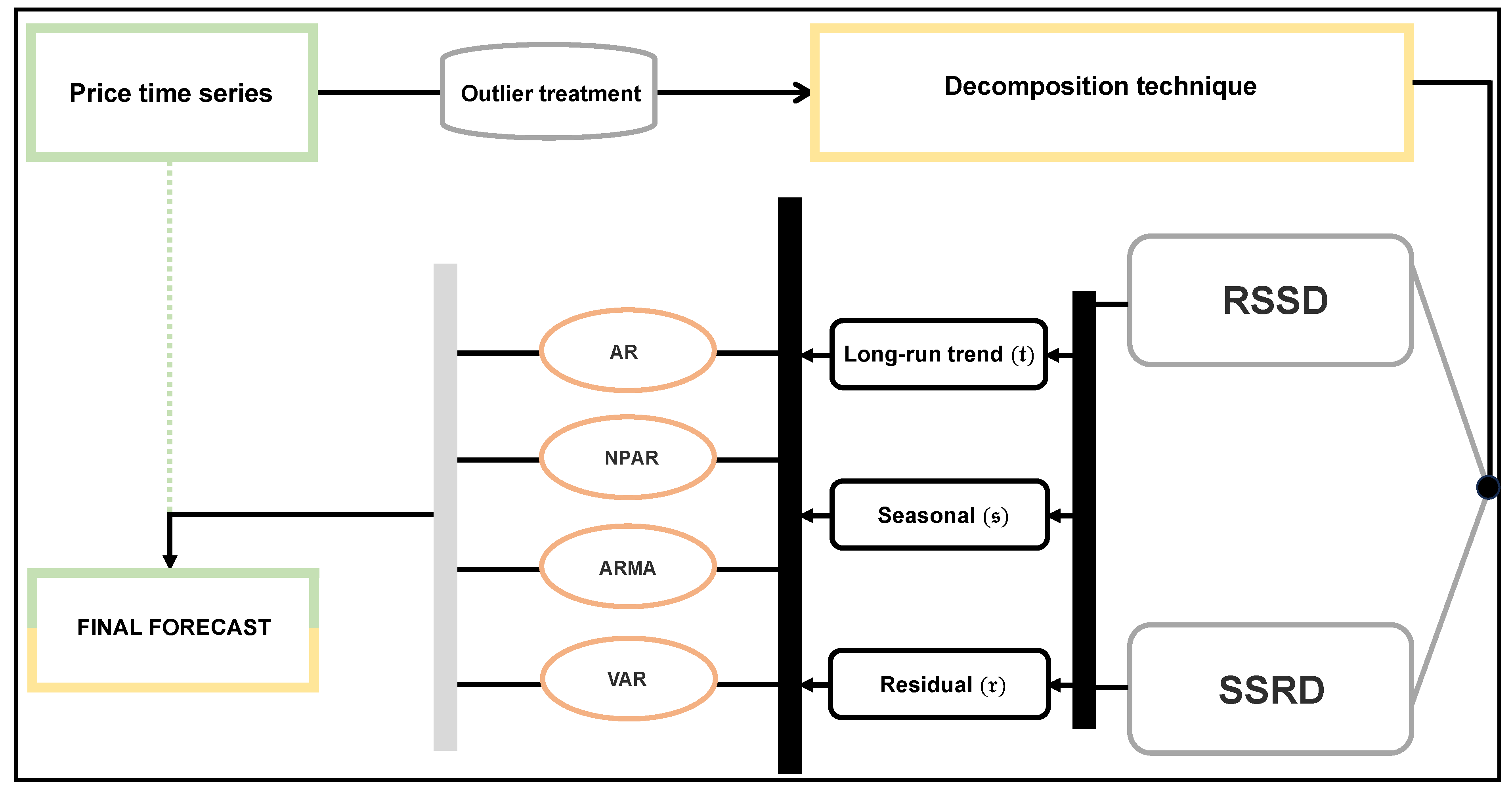
This section describes the general layout of the proposed decomposition–combination modeling and forecasting process for predicting day-ahead prices for electricity. However, the composition of the electricity price time-series is complex; they contain distinctive characteristics such as outliers (spikes or jumps), multiple seasonal periodicities (daily, weekly, quarterly, and annually), volatility, the effects of public holidays, and so on. Incorporating these distinctive characteristics into the model significantly improves forecast efficacy and accuracy. Hence, the first step is to use the recursive price filter to eliminate outliers (spikes or jumps) from the real electricity price time-series. The filtering of the original time-series of hourly electricity is detailed in depth in the following subsection:

2.1.1. Outliers Treatment

Before starting the modeling, it often makes sense to prepare the data. The goal of preprocessing is usually to simplify the modeling of the data. In the case of electricity prices, this process involves finding outliers (spikes or jumps) and treating those using standard techniques. In the literature on electricity prices, several outlier detection and imputation methods have been introduced [47,48,49]. To detect the outliers (jumps or peaks) in the original electricity price series in this work, we take the 99.7% price confidence interval (u ± 3 s) as the acceptable limit and assume values outside this limit as atypical values; if we take the mean of the time-series of the electricity prices “m” and the standard deviation “s”, then the 99.7% confidence interval is m ± 3 s. In practice, start with the first observation in the data and see if the price is outside the confidence interval. In this case, it is considered an outlier and will later be replaced by the price value at the range boundary. Please note that the standard deviation must be recalculated each time an outlier is detected. Because after replacing outliers with bounded values, the standard deviation decreases. After replacing the outliers with the corresponding limit values according to the procedure described above, we obtain the filter price series.

After obtaining the filtered electricity price series in the first step, the filtered electricity price time-series is decomposed into three subseries. The long-term trend series, a seasonal series, and a residual series are in the second step. In doing so, we employ the proposed decomposition methods discussed in the coming section:

2.1.2. The Proposed Decomposition Methods

In this section, we describe a general decomposition procedure for filtered electricity price time-series. Hence, the filtered electricity price series (${\mathfrak{f}}_{\mathrm{n}}$) is split into three new subseries. The long-term trend $\left({\mathfrak{t}}_{\mathrm{n}}\right)$ series, a seasonal $\left({\mathfrak{s}}_{\mathrm{n}}\right)$ series, and the residual $\left({\mathfrak{r}}_{\mathrm{n}}\right)$ series. The mathematical equation is given as

$${\mathfrak{f}}_{\mathrm{n}}={\mathfrak{t}}_{\mathrm{n}}+{\mathfrak{s}}_{\mathrm{n}}+{\mathfrak{r}}_{\mathrm{n}}$$

(1)

furthermore, the seasonal subseries, ${\mathfrak{s}}_{\mathrm{n}}$, is comprised of the weekly (${\mathfrak{w}}_{\mathrm{n}}$), and yearly (${\mathfrak{y}}_{\mathrm{n}}$) cycles, and is modeled as:

$${\mathfrak{s}}_{\mathrm{n}}={\mathfrak{w}}_{\mathrm{n}}+{\mathfrak{y}}_{\mathrm{n}}$$

(2)

please note that in the above equation, all series subscript n = 1, 2, …, N. Thus, for modeling and forecasting purposes, the long-term trend series ${\mathfrak{t}}_{\mathrm{n}}$ is a function of time n, the seasonal subseries ${\mathfrak{s}}_{\mathrm{n}}$, is encompassed of the weekly ${\mathfrak{w}}_{\mathrm{n}}$ and yearly ${\mathfrak{y}}_{\mathrm{n}}$ cycles, are the function of the series $(1,2,3,\dots ,7,1,2,3,\dots ,7,\dots )$, and $(1,2,3,\dots ,365,1,2,3,\dots ,365,\dots )$, and the residual (irregular) subseries derived by describing the short-run dependency of the electricity price time-series ${\mathfrak{r}}_{\mathrm{n}}={\mathfrak{f}}_{\mathrm{n}}-({\mathfrak{t}}_{\mathrm{n}}+{\mathfrak{s}}_{\mathrm{n}})$. Therefore, the proposed decomposition methods, which include regression splines decomposition (RSD) and smoothing splines decomposition (SSD), can be found below.

Regression Spline Decomposition Technique

Regression spline is a common nonparametric regression approach that uses q-order piecewise polynomials to approximate ${\mathfrak{f}}_{\mathrm{n}}$ and estimates on the subintervals limited by a series of n points (called knots) [50]. Any spline function $\mathfrak{u}\left(\mathfrak{f}\right)$ of order q may be defined as a linear combination of basis functions ${\mathfrak{u}}_{\mathfrak{i}}\left(\mathfrak{f}\right)$, and its mathematical equation is as follows:

$$\begin{array}{c}\hfill \mathfrak{u}\left(\mathfrak{f}\right)=\sum _{i=1}^{\mathrm{n}+\mathrm{q}+1}{\alpha }_i{\mathfrak{u}}_{\mathfrak{i}}\left(\mathfrak{f}\right)\end{array}$$

(3)

the ordinary least-squares approach is used to estimate the unknown parameters ${\alpha }_i$. However, the number of nodes and their positions, which define the smoothness of the approximation, is the most essential choices, which are determined using the cross-validation technique in this work.

Smoothing Splines Decomposition Technique

Alternatively, the spline function can be predicted using the penalized least-squares method, which limits the sum of squares to meet the requirements for solving the knotted region [50]. The mathematical formula is given as:

$$\sum _{j=1}^N{({\mathfrak{f}}_{\mathrm{n}}-\mathfrak{u}\left(\mathfrak{f}\right))}^2+\gamma \int {\left({\mathfrak{u}}^{″}\left(\mathfrak{f}\right)\right)}^{2}d\mathrm{n}$$

(4)

in the above mathematical formula, the $\left({\mathfrak{u}}^{″}\left(\mathfrak{f}\right)\right)$ is the second derivative of $\mathfrak{u}\left(\mathfrak{f}\right)$. The first term considers the degree of fitting, and the second term determines the coarseness of the function through the smoothing parameter $\gamma$. Moreover, the selection of smoothing parameters is a difficult task, but it is performed using cross-validation methods in this study.

2.1.3. Decomposed Subseries Modeling

Once the subseries is obtained using the proposed decomposition methods mentioned above, we estimate each subseries using various linear and nonlinear, univariate, and multivariate time-series models, including the autoregressive, nonparametric autoregressive, autoregressive moving average, and vector autoregressive. The details about these models are given in subsections.

Parametric Autoregressive Model

The parametric autoregressive (AR) model explains the short-term dynamics of ${\mathfrak{f}}_{\mathrm{n}}$ considers a linear combination of the past (n) observations of ${\mathfrak{f}}_{\mathrm{n}}$ [51]. The functional form of the AR model is the following:

$${\mathfrak{f}}_{\mathrm{n}}=\mathrm{I}+{\sum }_{i=1}^{\mathrm{r}}{\alpha }_i{\mathfrak{f}}_{\mathrm{n}-\mathfrak{i}}+{ϵ}_{\mathrm{n}}$$

(5)

in the above equation, the I is showing the intercept term; the ${\alpha }_i$ is the unknown parameter of the AR (r) model, where $(i=1,2,\dots ,\mathrm{r})$; and ${ϵ}_{\mathrm{n}}$ a white noise process. In the current work, the unknown parameters (${\alpha }_i$) are estimated by the maximum likelihood estimation method; after a graphical analysis of different loading periods for each subseries, the authors conclude that lags 1, 2, and 7 are significant in most cases.

Nonparametric Autoregressive Model

In a nonparametric autoregressive model (NPAR), the relationship between ${\mathfrak{f}}_{\mathrm{n}}$ and its lag values has no particular parametric form and can tolerate any kind of nonlinearity [52]. The formula of the NPAR is given as

$${\mathfrak{f}}_{\mathrm{n}}={\sum }_{i=1}^{\mathrm{r}}{\mathrm{h}}_i\left({\mathfrak{f}}_{\mathfrak{n}-\mathfrak{i}}\right)+{ϵ}_{\mathrm{n}}$$

(6)

where ${\mathrm{h}}_i$ are smoothing functions, which describe the relationship between each passed value and ${\mathfrak{f}}_{\mathrm{n}}$. In this work, cubic regression splines are used to represent the ${\mathrm{h}}_i$ functions. and as a parametric case, uses lags 1, 2, and 7 to estimate the NPAR model.

Autoregressive Moving Average Model

An autoregressive moving average (ARMA) model considers the past values of the series and the lagged series of the error term to the model. In the current study, subseries are modeled as a linear combination of past (r) observations and a linear combination of past (k) error terms [53]. Hence, the mathematical functional form is given by

$${\mathfrak{f}}_{\mathrm{n}}=\mathrm{I}+{\sum }_{i=1}^{\mathrm{r}}{\alpha }_i{\mathfrak{f}}_{\mathrm{n}-\mathfrak{i}}+{\sum }_{j=1}^{\mathrm{k}}{\phi }_j{ϵ}_{\mathrm{n}-\mathrm{k}}+{ϵ}_{\mathrm{n}}$$

(7)

in the above functional form, the I is showing the intercept term; the ${\alpha }_i$ is the unknown parameter of the AR (r) model, where $(i=1,2,\dots ,\mathrm{r})$; and the MA are components or ${ϵ}_n\sim \mathrm{N}(0,{\sigma }_{ϵ}^2)$. In this study, the graphical analyzes suggest that lags 1, 2, and 7 for the AR component are significant, while only lags 1 and 2 for the MA component, i.e., an ARMA (c(1,2,7),2) model with ${\alpha }_3=\cdots ={\alpha }_6=0$ corresponds to ${\mathfrak{f}}_{\mathrm{n}}$ by the maximum likelihood estimation method.

Vector Autoregressive Model

In parametric vector autoregressive (VAR) models, both the dependent (response) and independent (predictor) are vectors, so they contain information about the entire daily load profile. This way, potential dependencies between price ranks with different load times can be considered [54]. In this work, the decomposed subsequence is modeled as a linear combination of the last r observations of ${\mathfrak{f}}_{\mathrm{n}}$, i.e.,

$${\mathbf{f}}_{\mathrm{n}}={\sum }_{\mathbf{i}=\mathbf{1}}^{\mathrm{r}}{\mathbf{Q}}_{\mathbf{i}}{\mathfrak{f}}_{\mathrm{n}-\mathfrak{i}}+{ϵ}_{\mathrm{n}}$$

(8)

in the above formula, the ${\mathbf{f}}_{\mathrm{n}}=\{{\mathfrak{f}}_{\mathrm{h},\mathfrak{i}},\cdots ,{\mathfrak{f}}_{\mathfrak{24},\mathfrak{j}}\}$, ${\mathbf{Q}}_i$$(i=1,2,\dots ,\mathrm{r})$ are coefficient matrices and ${ϵ}_{\mathbf{n}}=({ϵ}_{1,i},\dots ,{ϵ}_{24,i})$ is a vector of the disturbance term, such that ${ϵ}_{\mathrm{n}}\sim \mathrm{N}(\mathbf{0},{\sum }_{ϵ})$. The unknown parameters of the model are estimated using the maximum likelihood estimation method.

In this work, for simplicity, we symbolize each combined model with each decomposition method: ${}^{\mathfrak{t}}$RSD${}_{\mathfrak{r}}^{\mathfrak{s}}$, top-left (long-run trend term), top-right (seasonal), and bottom-right (residual) subseries. Also, for the estimation model, we assign numbers to each model, e.g., parametric autoregressive (1), nonparametric autoregressive (2), autoregressive moving average (3), and vector autoregressive (4). For example, ${}^1$RSD${}_2^3$, indicates that the long run ($\mathfrak{t}$) by an autoregressive seasonal series ($\mathfrak{s}$) is estimated using the nonparametric autoregressive model, and the residual ($\mathfrak{r}$) is estimated using the autoregressive moving average model. To get the final day-ahead price forecast, the individual forecast models are linked directly to each other as follows:

$$\begin{array}{ccc}\hfill {\widehat{\mathfrak{f}}}_{\mathrm{n}+1}& =& \left({\widehat{\mathfrak{t}}}_{\mathrm{n}+1}+{\widehat{\mathfrak{s}}}_{\mathrm{n}+1}+{\widehat{\mathfrak{r}}}_{\mathrm{n}+1}\right)\hfill \\ & =& \left(\widehat{\widehat{}}{\mathfrak{t}}_{\mathrm{n}+1}+{\widehat{\mathfrak{y}}}_{\mathrm{n}+1}+{\widehat{\mathfrak{w}}}_{\mathrm{n}+1}+{\widehat{\mathfrak{r}}}_{\mathrm{n}+1}\right)\hfill \end{array}$$

(9)

2.2. Models Evaluation Measures

In the literature on forecasting models, various researchers have used different accuracy measures, a statistical test, and a graphic analysis to verify the performance of forecasting models [55,56]. However, in this work, to check the performance of the final models obtained from various linear and nonlinear, univariate and multivariate, and all possible combinations, four standard measures of precision comprising mean squared absolute percent error (MSPE), mean absolute error (MAE), root mean squared error (RMSE), and mean absolute percentage error (MAPE) were calculated. The mathematical equations for the mean errors are as follows:

$$\begin{array}{c}\hfill \mathrm{MSPE}=\frac{1}{\mathrm{N}}\sum _{\mathrm{n}=1}^{\mathrm{N}}{\left(\frac{|{\mathfrak{f}}_{\mathrm{n}}-{\widehat{\mathfrak{f}}}_{\mathrm{n}}|}{|{\mathfrak{f}}_{\mathrm{n}}|}\right)}^2\times 100,\end{array}$$

(10)

$$\begin{array}{c}\hfill \mathrm{MAE}=\frac{1}{\mathrm{N}}\sum _{\mathrm{n}=1}^{\mathrm{N}}\left(|{\mathfrak{f}}_{\mathrm{n}}-{\widehat{\mathfrak{f}}}_{\mathrm{n}}|\right),\end{array}$$

(11)

$$\begin{array}{c}\hfill \mathrm{RMSE}=\sqrt{\frac{1}{\mathrm{N}}\sum _{\mathrm{n}=1}^{\mathrm{N}}{({\mathfrak{f}}_{\mathrm{n}}-{\widehat{\mathfrak{f}}}_{\mathrm{n}})}^2},\end{array}$$

(12)

$$\begin{array}{c}\hfill \mathrm{MAPE}=\frac{1}{\mathrm{N}}\sum _{\mathrm{n}=1}^{\mathrm{N}}\left(\frac{|{\mathfrak{f}}_{\mathrm{n}}-{\widehat{\mathfrak{f}}}_{\mathrm{n}}|}{|{\mathfrak{f}}_{\mathrm{n}}|}\right)\times 100,\end{array}$$

(13)

where ${\mathfrak{f}}_{\mathrm{n}}$ is observed and ${\widehat{\mathfrak{f}}}_{\mathrm{n}}$ is forecasted price value for nth observation (n = 1, 2, …, N = 8760). In general, the lower the MSPE, MAPE, MAE, and RMSE, the higher the forecasting accuracy of the model.

In addition to the metrics mentioned above, the Diebold-Mariano (DM) [57] test is a commonly used statistical test for evaluating forecasts from different models in the electricity price and demand literature [58,59]. For instance, consider the two forecasts obtained from the two different time-series models, such as ${\widehat{\mathfrak{f}}}_{\mathfrak{1}\mathrm{n}}$ (model 1) and ${\widehat{\mathfrak{f}}}_{\mathfrak{2}\mathrm{n}}$ (model 2). However, ${\Gamma }_{1\mathrm{d}}={\mathfrak{f}}_{\mathrm{n}}-{\widehat{\mathfrak{f}}}_{\mathfrak{1}\mathrm{n}}$ and ${\Gamma }_{2\mathrm{n}}={\mathfrak{f}}_{\mathrm{n}}-{\widehat{\mathfrak{f}}}_{\mathfrak{2}\mathrm{n}}$ are the corresponding forecast errors. The loss associated with forecast error ${\left\{{\Gamma }_{\mathrm{i}\mathrm{n}}\right\}}_{\mathrm{i}=1}^2$ by $\eta \left({\Gamma }_{\mathrm{i}\mathrm{n}}\right)$. For example, time n absolute loss would be $\eta \left({\Gamma }_{\mathrm{i}\mathrm{n}}\right)=\left|{\Gamma }_{\mathrm{i}\mathrm{n}}\right|$. The loss resulting from Predictions 1 and 2, respectively, for time n, is thus ${\wp }_{\mathrm{n}}=\eta \left({\Gamma }_{1\mathrm{n}}\right)-\eta \left({\Gamma }_{2\mathrm{n}}\right)$. The null hypothesis with the same accuracy in forecasting for two predictions is $\mathrm{E}\left[{\wp }_{\mathrm{n}}\right]=0$. The DM test rules that the loss difference be covariance steady, i.e.,

$$\begin{array}{ccc}\hfill \mathrm{E}\left[{\wp }_{\mathrm{n}}\right]& =& \alpha ,\forall \mathrm{n}\hfill \end{array}$$

(14)

$$\begin{array}{ccc}\hfill \mathrm{cov}({\wp }_{\mathrm{n}}-{\wp }_{\mathrm{n}-\mathrm{n}})& =& \rho \left(\mathrm{n}\right),\forall \mathrm{n}\hfill \end{array}$$

(15)

$$\begin{array}{ccc}\hfill \mathrm{var}\left({\wp }_{\mathrm{n}}\right)& =& {\sigma }_{\wp },0<{\sigma }_{\wp }<\infty \hfill \end{array}$$

(16)

considering these assumptions, a DM test with equal prediction accuracy is

$$\begin{array}{c}\hfill \mathrm{DM}=\frac{\overline{\wp }}{{\widehat{\sigma }}_{\overline{\wp }}}\stackrel{\mathrm{n}}{\to }\mathrm{Norm}(0,1)\end{array}$$

(17)

in the above equation, $\overline{\wp }=\frac{1}{\mathrm{N}}{\sum }_{\mathrm{n}=1}^{\mathrm{N}}{\wp }_{\mathrm{n}}$ is the sample average loss differential and ${\widehat{\sigma }}_{\overline{\wp }}$ is a consistent standard error estimate of ${\wp }_{\mathrm{n}}$.

Finally, to verify the superiority of the proposed decomposition–combination approach using different figures, such as the box-plot, line-plot, bar-plot, and dot-plot in this work. To conclude this section, the design of the proposed decomposition–combination modeling and forecasting approach is shown in Figure 1.

3. Case Study Results

This research article primarily focuses on electricity price fluctuations before COVID-19. For this purpose, this work uses the hourly spot electricity prices (euro/MWh) from the Italian electricity market collected from 1 January 2014 to 31 December 2019. Each day consists of 24 data points, with each data point corresponding to a load period. Therefore, it corresponds to 52,584 data points (2191 days). We divided the data into two groups for modeling and forecasting motives: a training group (model estimation) and the validation group(out-of-sample forecast). The training part configured the data from 1 January 2014 to 31 December 2018 (1826 days or 43,824 observations), which is approximately 80% of the total data, and the period from 1 January 2019 to 31 December 2019 (365 days or 8760 observations) was used as the out-of-ample forecast. The one-day-ahead out-of-sample forecast is determined by the moving or rolling window method [60]. A rolling or moving window technique of analysis of a time-series model is often used to evaluate stability over time. When analyzing financial time-series data (energy prices) using statistical models, the main assumption is that the model parameters are unchanged over time. However, the economic environment often changes abruptly, and it may not be reasonable to assume that the parameters of a model are constant. A common technique to evaluate the constancy of model parameters is to compute parameter estimates over a fixed-size moving window over the sample. If the parameters are constant over the entire sample, the estimates on the sliding windows should not be too different. If the parameters change at some point during the sampling, then the alternate estimates will capture this instability.

However, this technique is one of the most popular methods for evaluating the accuracy and ability to forecast a statistical model using past data. This involves splitting the historical data into two sets: estimation and out-of-sample. The estimation set is used to develop the model and produce k-step-ahead (one-step-ahead in our case) projections for the out-of-sample set. However, the predictions may contain errors since the data used has already been observed. To address this, the estimation set is shifted by a set amount, and the process of estimation and out-of-sample is repeated until no further k-step predictions can be made. It is important to note that in this approach, the number of parameters used remains constant throughout the rolling window analysis.

To acquire the forecast of electricity prices one day ahead using the proposed modeling framework, the following steps must be followed: First, the recursive price filtering technique was used to identify and impute the outliers. However, the filtered electricity price is shown in Figure 2 (right) and the original Figure 2 (left). The visual representation indicates that the filtered price time-series has no more extremes than the original electricity price time-series. Also, the descriptive statistics, non-stationary statistics (augmented dickey-fuller (ADF) [61] and Phillips-Perron unit root (PP) [62] tests), and autoregressive conditional heteroskedasticity (ARCH) effect tests [63] (the Ljung-Box (Box) and the Lagrange Multiplier (LM) tests) for the original electricity prices time-series, the filtered prices time-series, and the log-filtered prices time-series are provided in

Table 1. IPEX electricity prices (euro/MWh): Descriptive statistics of the original prices and the time-series of filtered prices.

S. No	Measure	Original Series	Filtered Series	Log (Filtered Series)
1	Min	1.00	3.65	1.29
2	Q1	42.00	42.00	3.74
3	Median	50.00	50.00	3.91
4	Mean	51.98	51.88	3.91
5	Mode	50.00	50.00	3.91
6	Var	235.87	223.30	0.09
7	Sdv	15.36	14.94	0.30
8	Skewness	0.83	0.58	−0.75
9	Kurtosis	2.35	0.82	2.95
10	Q3	61.00	61.00	4.11
11	Max	170.00	115.21	4.75
12	ADF (Statistic)	−15.39	−15.03	−16.32
13	PP (Statistic)	−331.07	−310.68	−281.35
14	ARCH (BOX)	75,641.61	76,207.77	81,342.81
15	ARCH (LM)	−18,452.44	−19,221.19	−25,706.73

. Hence, descriptive metrics are a collection of methods for summarizing and describing the key characteristics of a dataset, such as its central tendency, variability, and distribution. These statistics give an overview of the data and aid in determining the presence of patterns and linkages. It can be seen from Table 1 that the minimum and maximum electricity prices, standard deviation, skewness, and kurtosis change before and after treating outliers, while the mean, mode, median, and first and third quartiles are the same. In the same way, the log-filtered series has the least descriptive statistic values.

In addition to the above, to check the unit root issue of the original electricity prices time-series, the filtered prices time-series, and the log-filtered prices time-series statistically by the ADF and PP tests. The results (statistic values) are listed in Table 1, which suggests that the log-filtered electricity prices time-series have a higher negative statistic value, which indicates that the series is stationary. Furthermore, two ARCH tests, including Box and LM, are performed to verify the time-varying phenomena in conditional volatility. The test statistic results are listed in Table 1. From this table, it can be observed that in both tests, the log-filtered series showed better results. Based on all these results, we will proceed with further modeling and forecasting purposes with the log-filtered series. In addition, it is confirmed in Table 1 that the results of the ARCH test show that all three series (the original, the filtered, and the log-filtered electricity price time-series) have an ARCH effect. To achieve it, the proposed forecasting methodology is processed as follows: As we know, the log-filtered electricity series is an hourly time-series, and generally, it contains many periodicities (hourly, weekly, and yearly), with a linear or nonlinear trend component. To do this, in this work, the hourly dynamics were captured by each load period being modeled separately [64].

In the second step, the proposed decomposition methods were used to obtain long-term (${\mathfrak{t}}_{\mathrm{n}}$), seasonal (${\mathfrak{s}}_{\mathrm{n}}$), and residuals (${\mathfrak{r}}_{\mathrm{n}}$) time subseries. Thus, a graphical representation of decomposed subseries is given in Figure 3 (left panel) and Figure 3 (right panel). In both panels, first, the filtered log price series; second, the long-trend ($\mathfrak{t}$); third, the seasonal ($\mathfrak{s}$) and fourth, the residual ($\mathfrak{r}$), respectively. For both figures, it can be seen that both methods, the RSD and the SSD, decomposed the real-time-series of electricity prices and adequately captured both the dynamics, i.e., the long-term trend component, and the seasonality (yearly and weekly), which adequately captured the series of electricity prices.

Finally, in the third step, previously outdated univariate and multivariate models were applied to each subseries. After modeling these decomposed series, we checked their residuals for ARCH effects, so there was no more evidence of an ARCH effect this time. Therefore, the estimation of models was made to obtain a one-day-ahead forecast for 365 days, which comprises 8760 data points, using the rolling window method. The Equation (9) was used to obtain the final day-ahead price forecasts.

In this empirical study, the decomposition of the hourly filtered electricity spot prices time-series (${\mathfrak{f}}_{\mathrm{n}}$) into new subseries containing the long-term trend (${\mathfrak{t}}_{\mathrm{n}}$), a seasonal (${\mathfrak{s}}_{\mathrm{n}}$), and a residual series (${\mathfrak{r}}_{\mathrm{n}}$) was obtained by two proposed decomposition methods. On the other side, all three subseries are estimated using four different linear and nonlinear, univariate, and multivariate time-series models, and all possible combinations are considered. Hence, combining the models for the subseries estimations leads us to compare 64 ($4^{{\mathrm{n}}_{\mathfrak{t}}}\times 4^{{\mathrm{n}}_{\mathfrak{s}}}\times 4^{{\mathrm{n}}_{\mathfrak{r}}}$ = 64) different combinations for one decomposition method. Consequently, for both decomposition methods, the RSD and the SSD, there are 128 (2 × 64) models. For these all one hundred and 28 models, one day-ahead out-of-sample forecast results (MAE, MSPE, MAPE, and RMSE) are listed in

Table 2. IPEX electricity prices (euro/MWh): One-day-ahead out-of-sample forecasting mean errors for all combination models using the RSD decomposition method.

C.No	Models	MSPE	MAE	RMSE	MAPE	C.No	Models	MSPE	MAE	RMSE	MAPE
1	${}^1$RSD${}_1^1$	3.3923	5.6389	7.1224	11.9395	33	${}^3$RSD${}_1^1$	3.3925	5.6391	7.1225	11.9400
2	${}^1$RSD${}_2^1$	3.3826	5.6125	7.0944	11.8903	34	${}^3$RSD${}_2^1$	3.3829	5.6127	7.0946	11.8908
3	${}^1$RSD${}_3^1$	2.4298	5.2338	6.5375	10.9147	35	${}^3$RSD${}_3^1$	2.4299	5.2339	6.5376	10.9151
4	${}^1$RSD${}_4^1$	2.9581	5.3948	6.8388	11.2389	36	${}^3$RSD${}_4^1$	2.9581	5.3950	6.8389	11.2393
5	${}^1$RSD${}_1^2$	2.2630	4.2231	5.5877	8.9818	37	${}^3$RSD${}_1^1$	2.2633	4.2232	5.5878	8.9821
6	${}^1$RSD${}_2^2$	2.3500	4.2336	5.5946	9.0085	38	${}^3$RSD${}_2^2$	2.3503	4.2337	5.5947	9.0089
7	${}^1$RSD${}_3^2$	1.4333	3.7416	4.9124	7.8360	39	${}^3$RSD${}_3^2$	1.4335	3.7416	4.9126	7.8362
8	${}^1$RSD${}_4^2$	1.7898	3.9726	5.2831	8.2834	40	${}^3$RSD${}_4^2$	1.7899	3.9726	5.2832	8.2835
9	${}^1$RSD${}_1^3$	2.8511	4.9314	6.3098	10.5257	41	${}^3$RSD${}_1^2$	2.8512	4.9316	6.3099	10.5262
10	${}^1$RSD${}_2^3$	2.8960	4.9297	6.3078	10.5286	42	${}^3$RSD${}_2^3$	2.8962	4.9299	6.3080	10.5291
11	${}^1$RSD${}_3^3$	1.9377	4.4911	5.7318	9.4305	43	${}^3$RSD${}_3^3$	1.9378	4.4912	5.7320	9.4308
12	${}^1$RSD${}_4^3$	2.3822	4.6377	5.9877	9.7289	44	${}^3$RSD${}_4^3$	2.3821	4.6378	5.9878	9.7292
13	${}^1$RSD${}_1^4$	2.2025	4.0659	5.4140	8.6634	45	${}^3$RSD${}_1^3$	2.2028	4.0660	5.4141	8.6638
14	${}^1$RSD${}_2^4$	2.2931	4.0810	5.4308	8.7015	46	${}^3$RSD${}_2^4$	2.2935	4.0812	5.4309	8.7019
15	${}^1$RSD${}_3^4$	1.3483	3.5880	4.7130	7.5116	47	${}^3$RSD${}_3^4$	1.3485	3.5881	4.7131	7.5119
16	${}^1$RSD${}_4^4$	1.7513	3.8620	5.1491	8.0601	48	${}^3$RSD${}_4^4$	1.7514	3.8621	5.1492	8.0603
17	${}^2$RSD${}_1^1$	3.3928	5.6394	7.1228	11.9402	49	${}^4$RSD${}_1^4$	3.4398	5.6619	7.1533	12.0069
18	${}^2$RSD${}_2^1$	3.3831	5.6128	7.0948	11.8905	50	${}^4$RSD${}_2^1$	3.4301	5.6384	7.1245	11.9630
19	${}^2$RSD${}_3^1$	2.4294	5.2335	6.5372	10.9139	51	${}^4$RSD${}_3^1$	2.4580	5.2720	6.5757	11.0002
20	${}^2$RSD${}_4^1$	2.9588	5.3953	6.8394	11.2396	52	${}^4$RSD${}_4^1$	2.9887	5.4327	6.8663	11.3297
21	${}^2$RSD${}_1^2$	2.2634	4.2242	5.5886	8.9836	53	${}^4$RSD${}_1^1$	2.3130	4.2687	5.6355	9.0926
22	${}^2$RSD${}_2^2$	2.3505	4.2345	5.5954	9.0100	54	${}^4$RSD${}_2^2$	2.3982	4.2750	5.6406	9.1118
23	${}^2$RSD${}_3^2$	1.4329	3.7415	4.9122	7.8358	55	${}^4$RSD${}_3^2$	1.4621	3.7954	4.9690	7.9494
24	${}^2$RSD${}_4^2$	1.7902	3.9736	5.2840	8.2853	56	${}^4$RSD${}_4^2$	1.8250	4.0215	5.3284	8.3954
25	${}^2$RSD${}_1^3$	2.8520	4.9322	6.3107	10.5272	57	${}^4$RSD${}_1^3$	2.8870	4.9605	6.3393	10.5928
26	${}^2$RSD${}_2^3$	2.8970	4.9306	6.3087	10.5301	58	${}^4$RSD${}_2^3$	2.9307	4.9567	6.3356	10.5926
27	${}^2$RSD${}_3^3$	1.9377	4.4912	5.7320	9.4306	59	${}^4$RSD${}_3^3$	1.9545	4.5296	5.7653	9.5072
28	${}^2$RSD${}_4^3$	2.3831	4.6386	5.9888	9.7305	60	${}^4$RSD${}_4^3$	2.4035	4.6649	6.0146	9.7882
29	${}^2$RSD${}_1^4$	2.2028	4.0668	5.4148	8.6652	61	${}^4$RSD${}_1^4$	2.2541	4.1137	5.4638	8.7776
30	${}^2$RSD${}_2^4$	2.2936	4.0817	5.4315	8.7027	62	${}^4$RSD${}_2^4$	2.3428	4.1277	5.4786	8.8144
31	${}^2$RSD${}_3^4$	1.3480	3.5880	4.7126	7.5116	63	${}^4$RSD${}_3^4$	1.3796	3.6441	4.7751	7.6319
32	${}^2$RSD${}_4^4$	1.7516	3.8630	5.1500	8.0619	64	${}^4$RSD${}_4^4$	1.7889	3.9093	5.1980	8.1688

and

Table 3. IPEX electricity prices (euro/MWh): One-day-ahead out-of-sample forecasting mean errors for all combination models using the SSD decomposition method.

C.No	Models	MSPE	MAE	RMSE	MAPE	C.No	Models	MSPE	MAE	RMSE	MAPE
1	${}^1$SSD${}_1^1$	4.3140	6.9554	8.6969	4.3140	33	${}^3$SSD${}_1^1$	4.3212	6.9605	8.7027	14.3541
2	${}^1$SSD${}_2^1$	3.2513	5.5656	7.0489	3.2513	34	${}^3$SSD${}_2^1$	3.2606	5.5714	7.0568	11.7561
3	${}^1$SSD${}_3^1$	2.3918	5.1927	6.5252	2.3918	35	${}^3$SSD${}_3^1$	2.3956	5.1966	6.5302	10.8470
4	${}^1$SSD${}_4^1$	2.8524	5.3475	6.7795	2.8524	36	${}^3$SSD${}_4^1$	2.8580	5.3535	6.7857	11.1413
5	${}^1$SSD${}_1^2$	2.8856	5.3405	6.7870	2.8856	37	${}^3$SSD${}_1^2$	2.8927	5.3458	6.7933	11.1627
6	${}^1$SSD${}_2^2$	2.3733	4.2349	5.6095	2.3733	38	${}^3$SSD${}_2^2$	2.3829	4.2410	5.6181	9.0278
7	${}^1$SSD${}_3^2$	1.5022	3.7722	4.9771	1.5022	39	${}^3$SSD${}_3^2$	1.5059	3.7761	4.9823	7.9674
8	${}^1$SSD${}_4^2$	1.8665	4.0023	5.3159	1.8665	40	${}^3$SSD${}_4^2$	1.8721	4.0086	5.3225	8.4070
9	${}^1$SSD${}_1^3$	3.5702	6.0681	7.6550	3.5702	41	${}^3$SSD${}_1^3$	3.5773	6.0733	7.6610	12.6325
10	${}^1$SSD${}_2^3$	2.9152	5.0163	6.4084	2.9152	42	${}^3$SSD${}_2^3$	2.9246	5.0225	6.4165	10.6697
11	${}^1$SSD${}_3^3$	1.9898	4.5644	5.8202	1.9898	43	${}^3$SSD${}_3^3$	1.9936	4.5689	5.8252	9.6093
12	${}^1$SSD${}_4^3$	2.4193	4.7235	6.0736	2.4193	44	${}^3$SSD${}_4^3$	2.4248	4.7300	6.0799	9.9112
13	${}^1$SSD${}_1^4$	2.7557	5.2929	6.6760	2.7557	45	${}^3$SSD${}_1^4$	2.7635	5.2984	6.6827	11.0104
14	${}^1$SSD${}_2^4$	2.2501	4.0996	5.4499	2.2501	46	${}^3$SSD${}_2^4$	2.2600	4.1060	5.4589	8.7303
15	${}^1$SSD${}_3^4$	1.4002	3.6463	4.7988	7.6716	47	${}^3$SSD${}_3^4$	1.4048	3.6511	4.8046	7.6859
16	${}^1$SSD${}_4^4$	1.7784	3.9017	5.1908	1.7784	48	${}^3$SSD${}_4^4$	1.7847	3.9082	5.1980	8.1800
17	${}^2$SSD${}_1^1$	4.3144	6.9554	8.6969	4.3144	49	${}^4$SSD${}_1^1$	4.3686	7.0032	8.7363	14.4589
18	${}^2$SSD${}_2^1$	3.2523	5.5660	7.0493	3.2523	50	${}^4$SSD${}_2^1$	3.2911	5.5874	7.0775	11.8027
19	${}^2$SSD${}_3^1$	2.3918	5.1928	6.5253	2.3918	51	${}^4$SSD${}_3^1$	2.4134	5.2316	6.5664	10.9169
20	${}^2$SSD${}_4^1$	2.8530	5.3480	6.7799	2.8530	52	${}^4$SSD${}_4^1$	2.8742	5.3832	6.8059	11.2048
21	${}^2$SSD${}_1^2$	2.8858	5.3406	6.7871	2.8858	53	${}^4$SSD${}_1^2$	2.9375	5.3867	6.8387	11.2577
22	${}^2$SSD${}_2^2$	2.3743	4.2357	5.6102	2.3743	54	${}^4$SSD${}_2^2$	2.4137	4.2687	5.6519	9.0929
23	${}^2$SSD${}_3^2$	1.5021	3.7722	4.9773	1.5021	55	${}^4$SSD${}_3^2$	1.5232	3.8307	5.0334	8.0710
24	${}^2$SSD${}_4^2$	1.8669	4.0032	5.3166	1.8669	56	${}^4$SSD${}_4^2$	1.8908	4.0417	5.3573	8.4748
25	${}^2$SSD${}_1^3$	3.5708	6.0681	7.6552	3.5708	57	${}^4$SSD${}_1^3$	3.6089	6.0972	7.6879	12.6948
26	${}^2$SSD${}_2^3$	2.9166	5.0167	6.4092	2.9166	58	${}^4$SSD${}_2^3$	2.9424	5.0353	6.4300	10.6980
27	${}^2$SSD${}_3^3$	1.9900	4.5647	5.8206	1.9900	59	${}^4$SSD${}_3^3$	2.0000	4.5977	5.8520	9.6589
28	${}^2$SSD${}_4^3$	2.4200	4.7241	6.0744	2.4200	60	${}^4$SSD${}_4^3$	2.4303	4.7452	6.0933	9.9389
29	${}^2$SSD${}_1^4$	2.7559	5.2927	6.6760	2.7559	61	${}^4$SSD${}_1^4$	2.8089	5.3388	6.7305	11.1066
30	${}^2$SSD${}_2^4$	2.2510	4.1003	5.4505	2.2510	62	${}^4$SSD${}_2^4$	2.2929	4.1419	5.4981	8.8115
31	${}^2$SSD${}_3^4$	1.4001	3.6465	4.7988	7.6859	63	${}^4$SSD${}_3^4$	1.4263	3.7083	4.8646	7.7992
32	${}^2$SSD${}_4^4$	1.7787	3.9025	5.1914	1.7787	64	${}^4$SSD${}_4^4$	1.8070	3.9471	5.2403	8.2561

. From Table 2, it is confirmed that the ${}^2$RSD${}_3^4$ combination model led to a better forecast compared to the rest of all combination models using the RSD method. The best forecasting model is obtained by ${}^2$RSD${}_3^4$, which produced 3.5880, 1.3480, 7.5116, and 4.7130 for MAE, MSPE, MAPE, and RMSE, respectively. Although the ${}^1$RSD${}_3^4$, ${}^3$RSD${}_3^4$ and ${}^4$RSD${}_3^4$ models produced the second, third, and fourth-best results within all 64 combination models using the RSD method. In the same way, from Table 3, one can see that the ${}^2$SSD${}_3^4$ combination model shows the best results compared to the rest of all 64 combination models using the SSD method. This best model obtained the following forecasting results: 3.5880, 1.3480, 7.5116, and 4.7130 for MAE, MSPE, MAPE, and RMSE, respectively. On the other hand, the ${}^1$SSD${}_3^4$, ${}^3$SSD${}_3^4$ and ${}^4$SSD${}_3^4$ models showed the second, third, and fourth-best results within all 64 combination models using the SSD method. When comparing the overall one hundred and 28 models from both decomposition methods, the RSD and SSD, the best one-day-ahead forecasting results were shown by the ${}^2$RSD${}_3^4$ combination model, while the second, third, and fourth-best results were within all one hundred and 28 combination models shown by the ${}^1$RSD${}_3^4$, ${}^3$RSD${}_3^4$ and ${}^4$RSD${}_3^4$ models. As a result of these results (accuracy mean errors), it is confirmed that, within the proposed decomposition methods, the RSD method shows high accuracy and efficiency in one-day-ahead electricity price forecasting. In contrast, the best combination model (${}^1$RSD${}_3^4$) shows high accuracy and efficiency in forecasting across all 128 models.

Similarly, from the proposed decomposition methods (RSD and SSD), the four best combination models from each decomposition method are selected and compared. For these 8 (4 × 2) best models, the mean accuracy errors are numerically tabulated in

Table 4. IPEX electricity prices (euro/MWh): the final best eight combination models day-ahead accuracy mean error results using the proposed RSD and SSD decomposition methods.

C.No	Models	MSPE	MAE	RMSE	MAPE
1	${}^1$RSD${}_3^4$	1.3483	3.5880	4.7130	7.5116
2	${}^2$RSD${}_3^4$	1.3480	3.5880	4.7126	7.5116
3	${}^3$RSD${}_3^4$	1.3485	3.5881	4.7131	7.5119
4	${}^4$RSD${}_3^4$	1.3796	3.6441	4.7751	7.6319
5	${}^2$SSD${}_3^4$	1.4001	3.6465	4.7988	7.6859
6	${}^1$SSD${}_3^4$	1.4002	3.6463	4.7988	7.6716
7	${}^3$SSD${}_3^4$	1.4048	3.6511	4.8046	7.6859
8	${}^4$SSD${}_3^4$	1.4263	3.7083	4.8646	7.7992

. It is confirmed that from this table, the ${}^2$RSD${}_3^4$ produced the smallest mean error values: RMSPE = 1.3480, MAPE = 7.5116, MAE = 3.5880, and RMSE = 4.7126, respectively. The ${}^1$RSD${}_3^4$, ${}^3$RSD${}_3^4$, and ${}^4$RSD${}_3^4$ showed the second, third, and fourth-best results in terms of accuracy mean errors. Thus, it is concluded that once again, within the proposed decomposition methods, the RSD decomposition method produced the lowest mean errors, and the ${}^2$RSD${}_3^4$ final super best combination model was considered the best model among the 12 best combination models.

After computing the mean errors, the next step is to identify the supremacy of these outcomes. This study used the DM test to validate the superiority of the final eight best combination models findings (mean errors) shown in Table 4. The outcomes (p-values) DM test are presented in

Table 5. IPEX electricity prices (euro/MWh): the DM test results (p-value) for the final best eight combination models using the proposed RSD and SSD decomposition methods (using the loss-squared function).

Models	${}^1$RSD${}_3^4$	${}^2$RSD${}_3^4$	${}^3$RSD${}_3^4$	${}^4$RSD${}_3^4$	${}^2$SSD${}_3^4$	${}^1$SSD${}_3^4$	${}^3$SSD${}_3^4$	${}^4$SSD${}_3^4$
${}^1$RSD${}_3^4$	0.000	0.198	0.156	0.975	0.010	0.009	0.006	0.582
${}^2$RSD${}_3^4$	0.802	0.000	0.109	0.975	0.011	0.010	0.006	0.588
${}^3$RSD${}_3^4$	0.844	0.891	0.000	0.976	0.011	0.010	0.006	0.590
${}^4$RSD${}_3^4$	0.025	0.025	0.024	0.000	0.002	0.002	0.001	0.012
${}^2$SSD${}_3^4$	0.990	0.989	0.989	0.998	0.000	0.123	0.021	0.973
${}^1$SSD${}_3^4$	0.991	0.990	0.990	0.998	0.877	0.000	0.054	0.974
${}^3$SSD${}_3^4$	0.994	0.994	0.994	0.999	0.979	0.946	0.000	0.985
${}^4$SSD${}_3^4$	0.418	0.412	0.410	0.988	0.027	0.026	0.015	0.000

. Compared to the alternate that each entry in Table 5 and the column/row predictive algorithms accuracy are higher compared to the row or column predictive scores for the hypothesis procedure, the null hypothesis cannot occur predictor. This table indicates that at the level of significance of 5%, the ${}^2$RSD${}_3^4$, ${}^1$RSD${}_3^4$, ${}^3$RSD${}_3^4$, and ${}^4$RSD${}_3^4$ models are statistically superior to the others among the best eight combination models in Table 4.

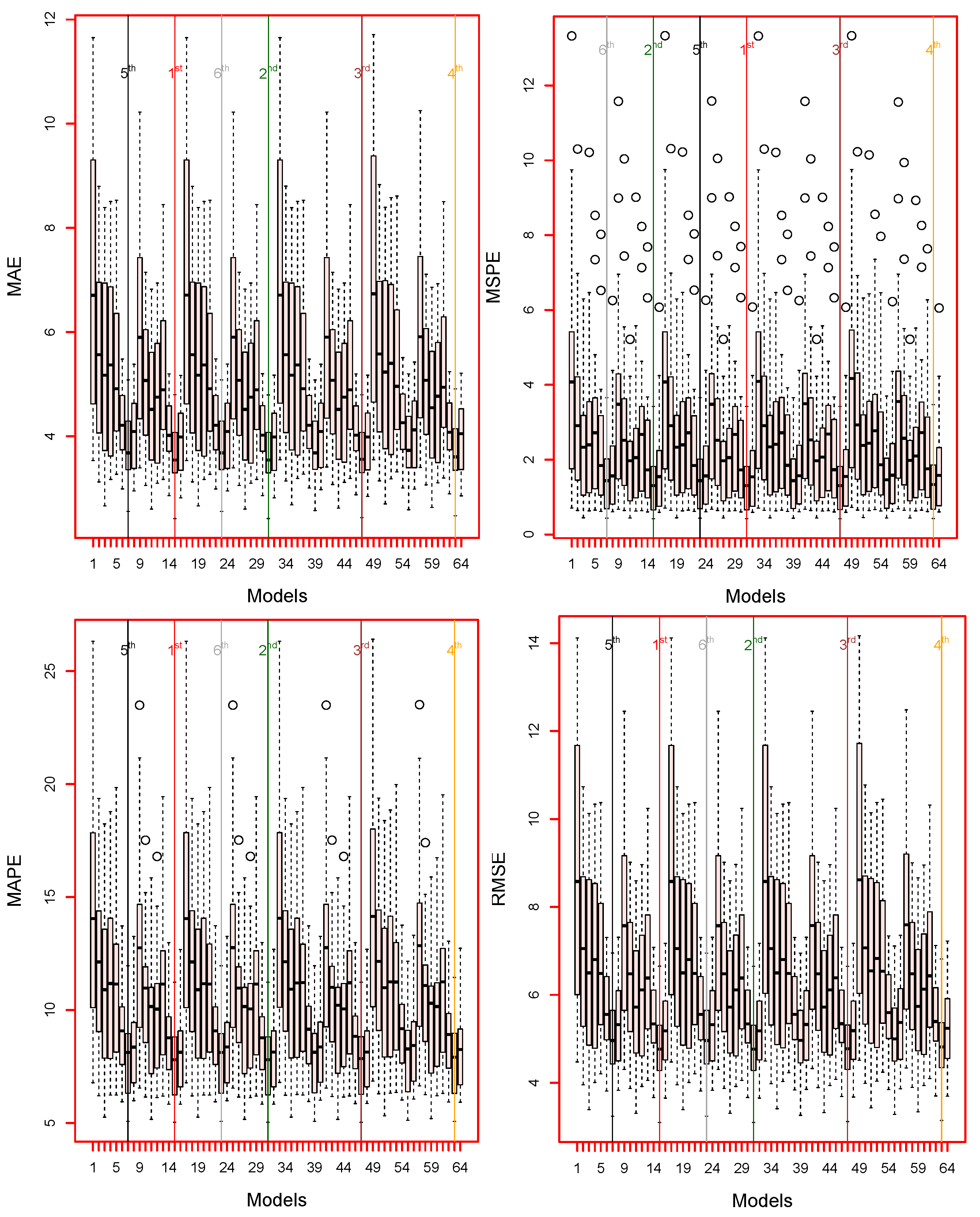
Finally, to verify the superiority of the proposed decomposition–combination approach using graphical analysis, including box plots, line plots, bar plots, and dot plots in this work. For example, the box plots of the MAE, MSPE, MAPE, and RMSE for all models (128) are given in Figure 4 and Figure 5. It can be seen from Figure 4; the smallest accuracy mean errors are produced by ${}^2$RSD${}_3^4$ combination models, while the ${}^1$RSD${}_3^4$, ${}^3$RSD${}_3^4$ and ${}^4$RSD${}_3^4$ combination models are second, third and fourth-best models, using the RSD method. In contrast, the results of the SSD method of the visual representation are shown in Figure 5; it is confirmed from these box plots that the lowest mean errors (MAE, MAPE, MSPE, and RMSE) values are obtained by ${}^2$SSD${}_3^4$ combination model, while the ${}^1$SSD${}_3^4$, ${}^3$SSD${}_3^4$ and ${}^4$SSD${}_3^4$ combination models, second, third, and fourth-best models. In the same way, from the proposed decomposition methods: RSD and SSD, the four best combination models from each decomposition method are selected and compared. For these 8 (4 × 2) best combination models, the mean accuracy errors are plotted in Figure 6. This figure shows that the ${}^2$RSD${}_3^4$ combination model obtained the lowest mean errors, while ${}^1$RSD${}_3^4$, ${}^3$RSD${}_3^4$ and ${}^4$RSD${}_3^4$ combination models are second, third and fourth-best results; in terms of accuracy mean errors comparing the eight best models form both proposed decomposition methods.

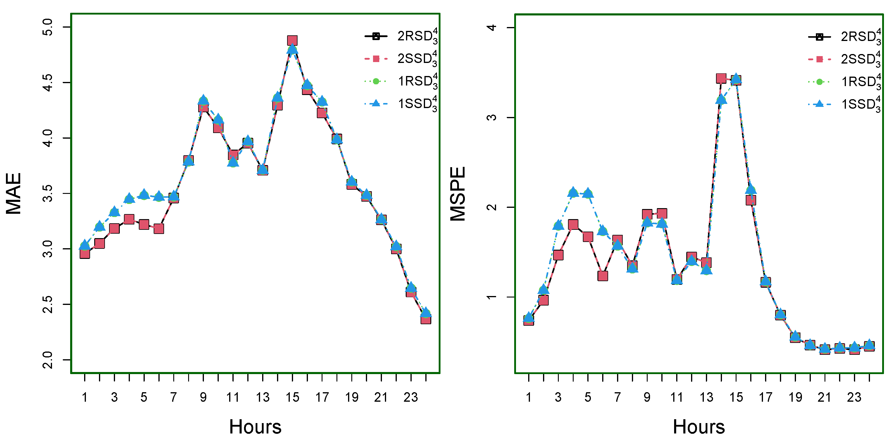
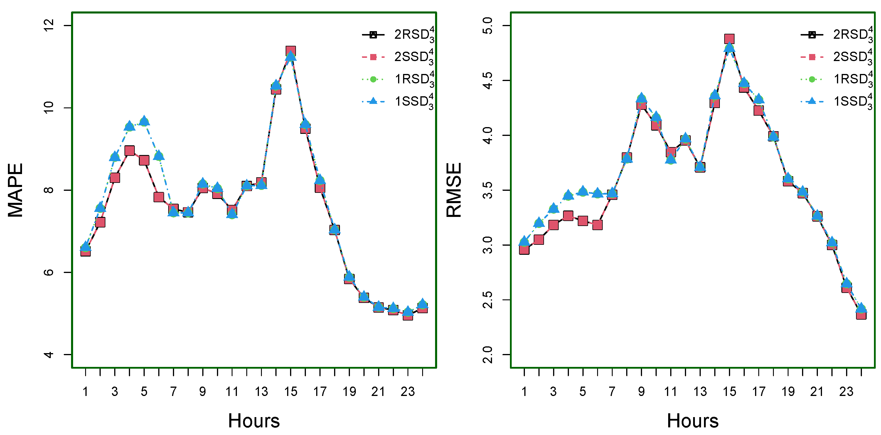
On the other hand, the hourly MAE, MSPE, MAPE, and RMSE for the super best four models among the eight best models, such as ${}^2$RSD${}_3^4$, ${}^1$RSD${}_3^4$, ${}^2$SSD${}_3^4$, and ${}^1$SSD${}_3^4$ are shown in Figure 7 for MAE (top-left), MSPE (top-right), MAPE (bottom-left), and RMSE (bottom-right). As of this figure, note that the hour means errors are lower at the start of the day and slowly increase with the first peak around 9:00 a.m.; after this, the values of mean errors are monotonically decreased and increase with the second peak around 3:00 p.m.

At the end of this section, the original and forecasted values for the best four combinations of models are ${}^2$RSD${}_3^4$, ${}^1$RSD${}_3^4$, ${}^2$SSD${}_3^4$, and ${}^1$SSD${}_3^4$, as shown in Figure 8. As confirmed by the figure, our model`s forecast follows observed prices very well. Therefore, we can determine that the ${}^2$RSD${}_3^4$, ${}^1$RSD${}_3^4$, ${}^2$SSD${}_3^4$, and ${}^1$SSD${}_3^4$, models outperformed the rest of them. Therefore, to conclude this section, from the accuracy mean errors (MSPE, MAPE, MAE, and RMSE), a statistical test (DM test), and graphical results (box-plot, bar-plot, and line plots), we can conclude that the proposed decomposition–combination forecasting methodology is highly efficient and accurate for one-day-ahead IPEX electricity prices. In addition, within the proposed all combination models, the ${}^2$RSD${}_3^4$ combination model produces more precise forecasts when compared with the alternative combinations.

At the end of this section, it is worth mentioning that all implementations were done using ‘R’, a language and environment for statistical computing. In more detail: Decomposition methods, modeling, and forecasting were implemented using the GAM library. The forecast, tsDyn, and vars libraries were used to estimate and forecast univariate and multivariate time-series models. In addition, all calculations were performed using an Intel (R) Core (TM) i5-6200U CPU at 2.40 GHz (Santa Clara, CA, USA).

4. Discussion

This section provides an overview of the comparison of the final best combination model (${}^2$RSD${}_3^4$) of this work with the literature’s best models and uses standard univariate and multivariate time-series benchmark models. Hence, in

Table 6. IPEX electricity prices (euro/MWh): Day-ahead Accuracy Mean Errors of the Proposed versus the Literature.

Models	MSPE	MAE	RMSE	MAPE
${}^4$RSD${}_3^4$	1.3480	3.5880	4.7130	7.5120
Sotc-AR [65]	4.1204	5.9122	7.2821	12.0175
Esamble [35]	3.9817	5.0600	6.6640	10.4516
NPAR [66]	4.9121	4.1061	6.8534	10.9031
MFP (VAR) [47]	3.1307	4.3171	6.5699	9.9359

numerically and graphically in Figure 9, an empirical comparison of our best combination model (${}^2$RSD${}_3^4$) with other researchers’ proposed models is presented. For example, It can be seen from these presentations that the best-proposed model (Stoc-AR) of [65] was applied to this work’s dataset, and their accuracy mean errors were obtained. The best-proposed model (Stoc-AR) of [65] reported the accuracy mean error values as the following: MSPE = 4.1204, MAE = 5.9122, RMSE = 7.2821, and MAPE = 12.0175, respectively, which are remarkable greater than our accuracy mean error values: MSPE = 1.3480, MAE = 3.5880, RMSE = 4.7130, and MAPE = 7.5120. In another work, ref. [66], the best-proposed model (NPAR) used the current study dataset and obtained performance measures that were comparatively higher than our best combination model. In the same way, for instance, the obtained forecasting mean errors by the best model [66] are the following: 4.9121, 4.1061, 6.8534, and 10.9031, which are significantly higher than our best combination model forecasting mean errors. In addition, in ref. [47], the best-proposed model (MPF-VAR) used the current study dataset and computed the accuracy measures that were also comparatively higher than our best model. To sum up, it can be seen that the best combination model of this work significantly obtained high accuracy as compared to the literature’s best models.

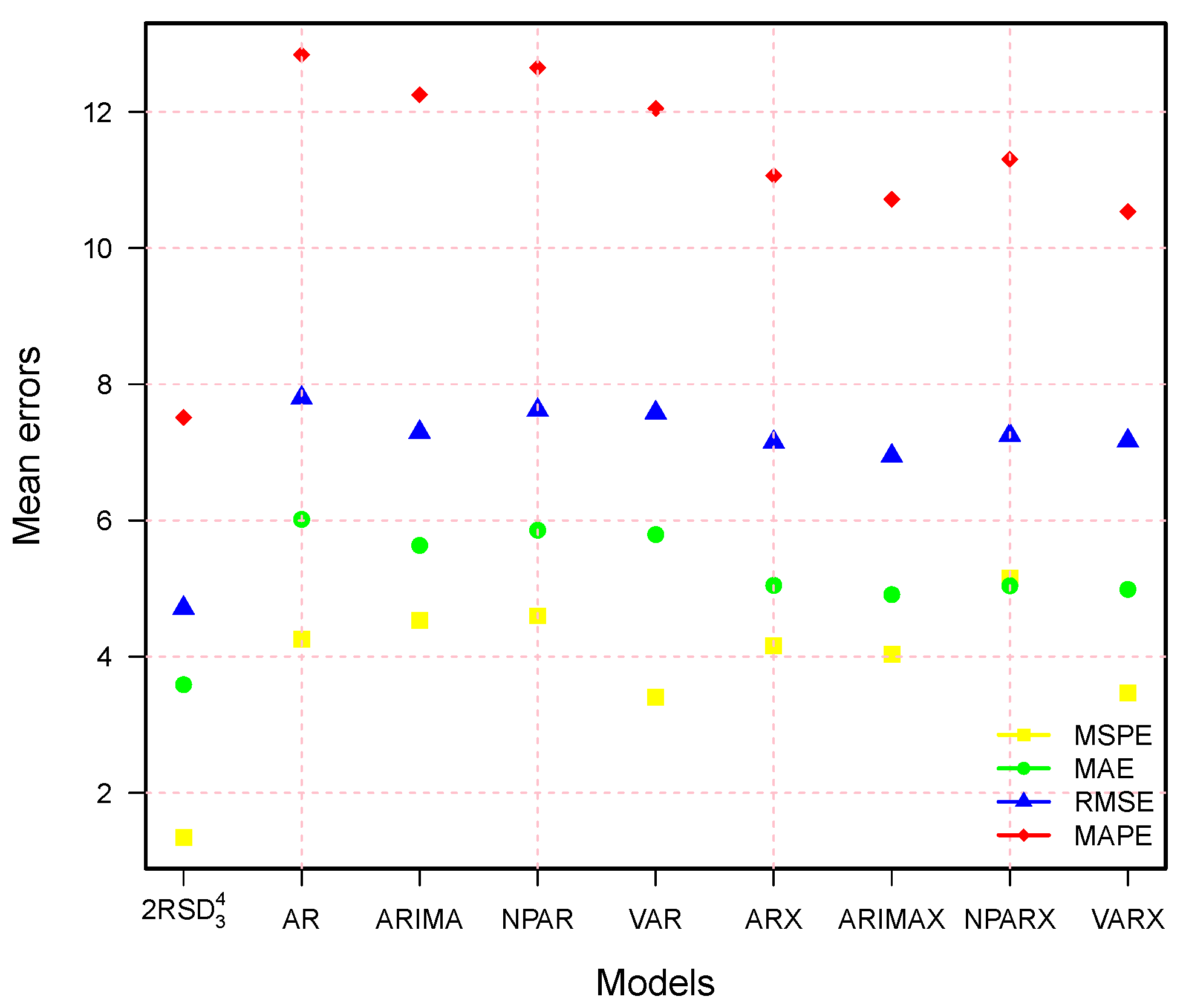
On the other hand, to assess the performance of our best combination model (${}^2$RSD${}_3^4$), it is compared to the standard benchmark univariate and multivariate time-series models: AR, ARIMA, NPAR, VAR, ARX, ARIMAX, NPARX, and VARX. In these models, X denotes the deterministic components, including a linear or nonlinear trend component, an annual cycle dummy, and a weekly period dummy. Therefore, the comparison results (numerically and graphically) are presented in

Table 7. IPEX electricity prices (euro/MWh): Day-ahead Accuracy Mean Errors of the Proposed versus the Benchmarks.

Models	MSPE	MAE	RMSE	MAPE
${}^4$RSD${}_3^4$	1.3480	3.5880	4.7130	7.5120
AR	4.2604	6.0152	7.7982	12.8395
ARIMA	4.5302	5.6337	7.2957	12.2521
NPAR	4.5985	5.8564	7.6187	12.6506
VAR	3.4064	5.7924	7.5807	12.0497
ARX	4.1588	5.0462	7.1494	11.0657
ARIMX	4.0314	4.9109	6.9465	10.7136
NPARX	5.1529	5.0411	7.2533	11.3038
VARX	3.4647	4.9870	7.1692	10.5359

and Figure 10. In these presentations, one can easily see that all benchmark models (AR, ARIMA, NPAR, VAR, ARX, ARIMAX, NPARX, and VARX) are outperformed by this work’s best model (${}^2$RSD${}_3^4$). Although the ARX, ARIMAX, NPARX, and VARX models show the best results compared to the models without deterministic components (AR, ARIMA, NPAR, and VAR), they still show the worst results compared to our best model. Thus, we can say that the best combination model in this study achieved significantly higher accuracy compared to all other benchmark models.

In summary, from the comparison results of the proposed best model from the literature and the recommended standard time-series model, the proposed best combination model has high efficiency and high efficiency for predicting the one-day-ahead electricity price of IPEX in this work. However, short-term accurate and efficient forecasts will help sellers (buyers and suppliers) optimize their bidding strategies, maximize profits, and use the resources needed to generate electricity more effectively. This also benefits the end user in terms of a reliable and economical energy system. In addition, good forecasts and knowledge of electricity price trends in developed and developing economies can help traders make more profitable business and trading plans and make beneficial asset allocation decisions. In addition, based on the best-proposed model, the sellers (buyers and suppliers) can develop a more robust trading plan and choose the model with the best risk-reward combination.

On the other hand, this study only utilizes data on electricity prices in Italy; however, it has the potential to be expanded to include other countries (the United States, the United Kingdom, the Nordic countries, Australia, Brazil, Chile, Peru, etc.) and energy market variables (electricity demand, electricity curves, natural gas prices, crude oil prices, etc.). This will allow for a more comprehensive evaluation of the effectiveness of the proposed decomposition methods in combination with the proposed forecasting methodology. In addition, the nonparametric regression methods (regression splines and smoothing splines) used in the proposed decomposition methods are adaptable to different data patterns, such as long-term linear or nonlinear trends, various periodicities (yearly, seasonal, weekly, and daily), non-constant mean and variance, jumps or peaks (extreme values), high volatility, calendar effects, and a tendency to return to average levels. These are achieved through the tuning of knots and sparsity levels.

5. Conclusions and Future Work Directions

Day-ahead electricity price forecasts have been crucial for market participants to optimize their strategies in today’s liberalized power market. Electricity prices, on the other hand, have unique characteristics such as long-term trends (linear or nonlinear), multiple periodicities (daily, weekly, quarterly, yearly), volatility, outliers (spikes or jumps), and holiday effects. These unique properties make the prediction problem a major challenge for researchers. Hence, incorporating these unique features into the model significantly increases forecast efficacy and accuracy. For this purpose, this work proposes a novel decomposition–combination technique to forecast day-ahead electricity prices. To this end, first, remove the outliers or spikes from the original electricity price time-series using the recursive price filter. Second, the filtered series of electricity prices was decomposed into three new subseries using the two proposed decomposition methods, such as a long-term trend series, a seasonal series, and a residual series. Third, forecast each subseries using different univariate and multivariate time-series models and all possible combinations. Finally, the individual forecasting models are combined directly to obtain the final one-day-ahead price forecast. The proposed decomposition–combination forecasting technique is applied to hourly spot electricity prices from Italian electricity-market data from 1 January 2014 to 31 December 2019. Hence, to check the performance of the proposed decomposition–combination modeling and forecasting technique, four different accuracy mean errors, including mean absolute error, mean square percentage error, mean absolute percentage error, and mean square error; a statistical test, the Diebold–Marino test; and a graphical analysis were considered. The empirical outcomes showed the efficiency and accuracy of the proposed method. Additionally, our forecasting outcomes were comparable to those described in the literature and were regarded as standard benchmark models. Finally, the authors recommended that the proposed decomposition–combination forecasting technique in this research work be applied to other complicated energy market forecasting challenges.

The main limitation of this research work is that it only considers hourly electricity prices; it can be extended to include other exogenous variables, such as electricity demand, temperature, natural gas prices, oil prices, coal prices, etc., which can improve electricity price forecasting. However, the current study uses only the IPEX dataset; it may be extended to other electricity markets, such as Nord Pool, PJM, AEM, etc., to evaluate the performance of the proposed decomposition–combination method in the future. On the other hand, only linear and nonlinear, univariate, and multivariate time-series models were used in the present study. Machine learning models such as deep learning and artificial neural networks can also be considered part of the current forecasting decomposition–combination technique. It can also be extended and applied to other approaches and datasets (for example, energy [1,3], air pollution [67,68,69,70], solid waste [71] and academic performance [72]).

References

1. López-Gonzales, J.L.; Castro Souza, R.; Leite Coelho da Silva, F.; Carbo-Bustinza, N.; Ibacache-Pulgar, G.; Calili, R.F. Simulation of the Energy Efficiency Auction Prices via the Markov Chain Monte Carlo Method. Energies 2020, 13, 4544. [Google Scholar] [CrossRef]
2. Iftikhar, H. Modeling and Forecasting Complex Time Series: A Case of Electricity Demand. Master’s Thesis, Quaid-i-Azam University, Islamabad, Pakistan, 2018. Available online: https://www.researchgate.net/publication/372103958_Modeling_and_Forecasting_Complex_Time_Series_A_Case_of_Electricity_Demand (accessed on 28 July 2023).
3. Gonzales, J.; Calili, R.; Souza, R.; Coelho da Silva, F. Simulation of the energy efficiency auction prices in Brazil. Renew. Energy Power Qual. J. 2016, 1, 574–579. [Google Scholar] [CrossRef]
4. Sulandari, W.; Lee, M.H.; Rodrigues, P.C. Indonesian electricity load forecasting using singular spectrum analysis, fuzzy systems and neural networks. Energy 2020, 190, 116408. [Google Scholar] [CrossRef]
5. Sulandari, W.; Yudhanto, Y.; Rodrigues, P.C. The use of singular spectrum analysis and k-means clustering-based bootstrap to improve multistep ahead load forecasting. Energies 2022, 15, 5838. [Google Scholar] [CrossRef]
6. Sulandari, W.; Subanar, S.; Lee, M.H.; Rodrigues, P.C. Time series forecasting using singular spectrum analysis, fuzzy systems and neural networks. MethodsX 2020, 7, 101015. [Google Scholar] [CrossRef] [PubMed]
7. Sulandari, W.; Subanar, S.; Suhartono, S.; Utami, H.; Lee, M.H.; Rodrigues, P.C. SSA based hybrid forecasting models and applications. Bull. Electr. Eng. Inform. 2020, 9, 2178–2188. [Google Scholar] [CrossRef]
8. Weron, R.; Bierbrauer, M.; Trück, S. Modeling electricity prices: Jump diffusion and regime switching. Phys. A Stat. Mech. Its Appl. 2004, 336, 39–48. [Google Scholar] [CrossRef]
9. Shah, I.; Iftikhar, H.; Ali, S. Modeling and forecasting medium-term electricity consumption using component estimation technique. Forecasting 2020, 2, 163–179. [Google Scholar] [CrossRef]
10. Lisi, F.; Nan, F. Component estimation for electricity prices: Procedures and comparisons. Energy Econ. 2014, 44, 143–159. [Google Scholar] [CrossRef]
11. Monteiro, C.; Ramirez-Rosado, I.J.; Fernandez-Jimenez, L.A.; Conde, P. Short-term price forecasting models based on artificial neural networks for intraday sessions in the Iberian electricity market. Energies 2016, 9, 721. [Google Scholar] [CrossRef]
12. Bildirici, M.; Ersin, Ö.Ö. Improving forecasts of GARCH family models with the artificial neural networks: An application to the daily returns in Istanbul Stock Exchange. Expert Syst. Appl. 2009, 36, 7355–7362. [Google Scholar] [CrossRef]
13. Makridakis, S.; Spiliotis, E.; Assimakopoulos, V. Statistical and Machine Learning forecasting methods: Concerns and ways forward. PLoS ONE 2018, 13, e0194889. [Google Scholar] [CrossRef] [PubMed]
14. de Marcos, R.A.; Bello, A.; Reneses, J. Electricity price forecasting in the short term hybridising fundamental and econometric modelling. Electr. Power Syst. Res. 2019, 167, 240–251. [Google Scholar] [CrossRef]
15. Olivares, K.G.; Challu, C.; Marcjasz, G.; Weron, R.; Dubrawski, A. Neural basis expansion analysis with exogenous variables: Forecasting electricity prices with NBEATSx. Int. J. Forecast. 2023, 39, 884–900. [Google Scholar] [CrossRef]
16. Shah, I.; Iftikhar, H.; Ali, S. Modeling and forecasting electricity demand and prices: A comparison of alternative approaches. J. Math. 2022, 2022, 3581037. [Google Scholar] [CrossRef]
17. Jan, F.; Shah, I.; Ali, S. Short-Term Electricity Prices Forecasting Using Functional Time Series Analysis. Energies 2022, 15, 3423. [Google Scholar] [CrossRef]
18. JSulandari, W.; Suhartono, S.; Subanar, S.; Rodrigues, P.C. Exponential smoothing on modelling and forecasting multiple seasonal time series: An overview. Fluct. Noise Lett. 2021, 20, 2130003. [Google Scholar] [CrossRef]
19. Nogales, F.J.; Contreras, J.; Conejo, A.J.; Espínola, R. Forecasting next-day electricity prices by time series models. IEEE Trans. Power Syst. 2002, 17, 342–348. [Google Scholar] [CrossRef]
20. Diongue, A.K.; Guegan, D.; Vignal, B. Forecasting electricity spot market prices with a k-factor GIGARCH process. Appl. Energy 2008, 96, 505–510. [Google Scholar] [CrossRef]
21. Weron, R.; Misiorek, A. Forecasting spot electricity prices: A comparison of parametric and semiparametric time series models. Int. J. Forecast. 2008, 24, 744–763. [Google Scholar] [CrossRef]
22. Girish, G.P. Spot electricity price forecasting in Indian electricity market using autoregressive-GARCH models. Energy Strategy Rev. 2016, 11, 52–57. [Google Scholar] [CrossRef]
23. Qu, H.; Duan, Q.; Niu, M. Modeling the volatility of realized volatility to improve volatility forecasts in electricity markets. Energy Econ. 2018, 74, 767–776. [Google Scholar] [CrossRef]
24. Bildirici, M.; Ersin, Ö. Modeling Markov switching ARMA-GARCH neural networks models and an application to forecasting stock returns. Sci. World J. 2014, 2014, 497941. [Google Scholar] [CrossRef] [PubMed]
25. Shah, I.; Bibi, H.; Ali, S.; Wang, L.; Yue, Z. Forecasting One-Day-Ahead Electricity Prices for Italian Electricity Market Using Parametric and Nonparametric Approaches. IEEE Access 2020, 8, 123104–123113. [Google Scholar] [CrossRef]
26. Carpio, J.; Juan, J.; López, D. Multivariate exponential smoothing and dynamic factor model applied to hourly electricity price analysis. Technometrics 2014, 56, 494–503. [Google Scholar] [CrossRef]
27. Taylor, J.W.; McSharry, P.E. Short-term load forecasting methods: An evaluation based on european data. IEEE Trans. Power Syst. 2007, 22, 2213–2219. [Google Scholar] [CrossRef]
28. De Livera, A.M.; Hyndman, R.J.; Snyder, R.D. Forecasting time series with complex seasonal patterns using exponential smoothing. J. Am. Stat. Assoc. 2011, 106, 1513–1527. [Google Scholar] [CrossRef]
29. Trull, O.; García-Díaz, J.C.; Troncoso, A. Initialization Methods for Multiple Seasonal Holt–Winters Forecasting Models. Mathematics 2020, 8, 268. [Google Scholar] [CrossRef]
30. Ahmed, M.I.; Kumar, R. Nodal Electricity Price Forecasting using Exponential Smoothing and Holt’s Exponential Smoothing. Distrib. Gener. Altern. Energy J. 2023, 38, 1505–1530. [Google Scholar] [CrossRef]
31. Tschora, L.; Pierre, E.; Plantevit, M.; Robardet, C. Electricity price forecasting on the day-ahead market using machine learning. Appl. Energy 2022, 313, 118752. [Google Scholar] [CrossRef]
32. Gholipour Khajeh, M.; Maleki, A.; Rosen, M.A.; Ahmadi, M.H. Electricity price forecasting using neural networks with an improved iterative training algorithm. Int. J. Ambient Energy 2018, 39, 147–158. [Google Scholar] [CrossRef]
33. Ugurlu, U.; Oksuz, I.; Tas, O. Electricity price forecasting using recurrent neural networks. Energies 2018, 11, 1255. [Google Scholar] [CrossRef]
34. Yang, W.; Sun, S.; Hao, Y.; Wang, S. A novel machine learning-based electricity price forecasting model based on optimal model selection strategy. Energy 2022, 238, 121989. [Google Scholar] [CrossRef]
35. Bibi, N.; Shah, I.; Alsubie, A.; Ali, S.; Lone, S.A. Electricity Spot Prices Forecasting Based on Ensemble Learning. IEEE Access 2021, 9, 150984–150992. [Google Scholar] [CrossRef]
36. Ersin, Ö.Ö.; Bildirici, M. Financial Volatility Modeling with the GARCH-MIDAS-LSTM Approach: The Effects of Economic Expectations, Geopolitical Risks and Industrial Production during COVID-19. Mathematics 2023, 11, 1785. [Google Scholar] [CrossRef]
37. Angamuthu Chinnathambi, R.; Mukherjee, A.; Campion, M.; Salehfar, H.; Hansen, T.M.; Lin, J.; Ranganathan, P. A multi-stage price forecasting model for day-ahead electricity markets. Forecasting 2018, 1, 26–46. [Google Scholar] [CrossRef]
38. Zhang, T.; Tang, Z.; Wu, J.; Du, X.; Chen, K. Short term electricity price forecasting using a new hybrid model based on two-layer decomposition technique and ensemble learning. Electr. Power Syst. Res. 2022, 205, 107762. [Google Scholar] [CrossRef]
39. Ribeiro, M.H.D.M.; Stefenon, S.F.; de Lima, J.D.; Nied, A.; Mariani, V.C.; Coelho, L.d.S. Electricity price forecasting based on self-adaptive decomposition and heterogeneous ensemble learning. Energies 2020, 13, 5190. [Google Scholar] [CrossRef]
40. Iftikhar, H.; Bibi, N.; Rodrigues, P.C.; López-Gonzales, J.L. Multiple Novel Decomposition Techniques for Time Series Forecasting: Application to Monthly Forecasting of Electricity Consumption in Pakistan. Energies 2023, 16, 2579. [Google Scholar] [CrossRef]
41. Yang, H.; Schell, K.R. GHTnet: Tri-Branch deep learning network for real-time electricity price forecasting. Energy 2022, 238, 122052. [Google Scholar] [CrossRef]
42. Yang, W.; Wang, J.; Niu, T.; Du, P. A hybrid forecasting system based on a dual decomposition strategy and multi-objective optimization for electricity price forecasting. Appl. Energy 2019, 235, 1205–1225. [Google Scholar] [CrossRef]
43. Zhang, J.; Tan, Z.; Wei, Y. An adaptive hybrid model for short term electricity price forecasting. Appl. Energy 2020, 258, 114087. [Google Scholar] [CrossRef]
44. Qiao, W.; Yang, Z. Forecast the electricity price of US using a wavelet transform-based hybrid model. Energy 2020, 193, 116704. [Google Scholar] [CrossRef]
45. Zhang, X.; Wang, J.; Gao, Y. A hybrid short-term electricity price forecasting framework: Cuckoo search-based feature selection with singular spectrum analysis and SVM. Energy Econ. 2019, 81, 899–913. [Google Scholar] [CrossRef]
46. Yang, W.; Wang, J.; Niu, T.; Du, P. A novel system for multi-step electricity price forecasting for electricity market management. Appl. Soft Comput. 2020, 88, 106029. [Google Scholar] [CrossRef]
47. Shah, I.; Akbar, S.; Saba, T.; Ali, S.; Rehman, A. Short-term forecasting for the electricity spot prices with extreme values treatment. IEEE Access 2021, 9, 105451–105462. [Google Scholar] [CrossRef]
48. Trueck, S.; Weron, R.; Wolff, R. Outlier Treatment and Robust Approaches for Modeling Electricity Spot Prices; Wrocław University of Technology: Wrocław, Poland, 2007. [Google Scholar]
49. Wang, J.; Yang, W.; Du, P.; Niu, T. Outlier-robust hybrid electricity price forecasting model for electricity market management. J. Clean. Prod. 2020, 249, 119318. [Google Scholar] [CrossRef]
50. James, G.; Witten, D.; Hastie, T.; Tibshirani, R. An Introduction to Statistical Learning; Springer: Berlin/Heidelberg, Germany, 2013; Volume 112. [Google Scholar]
51. Brockwell, P.J.; Davis, R.A. Introduction to Time Series and Forecasting; Springer Publication: Berlin/Heidelberg, Germany, 2016. [Google Scholar]
52. Wasserman, L. All of Nonparametric Statistics; Springer Science & Business Media: Berlin/Heidelberg, Germany, 2006. [Google Scholar]
53. Iftikhar, H.; Zafar, A.; Turpo-Chaparro, J.E.; Rodrigues, P.C.; López-Gonzales, J.L. Forecasting Day-Ahead Brent Crude Oil Prices Using Hybrid Combinations of Time Series Models. Mathematics 2023, 16, 3548. [Google Scholar] [CrossRef]
54. Hyndman, R.J.; Athanasopoulos, G. Forecasting: Principles and Practice; OTexts: Melbourne, Australia, 2018. [Google Scholar]
55. Iftikhar, H.; Khan, M.; Khan, Z.; Khan, F.; Alshanbari, H.M.; Ahmad, Z. A Comparative Analysis of Machine Learning Models: A Case Study in Predicting Chronic Kidney Disease. Sustainability 2023, 15, 2754. [Google Scholar] [CrossRef]
56. Alshanbari, H.M.; Iftikhar, H.; Khan, F.; Rind, M.; Ahmad, Z.; El-Bagoury, A.A.A.H. On the Implementation of the Artificial Neural Network Approach for Forecasting Different Healthcare Events. Diagnostics 2023, 13, 1310. [Google Scholar] [CrossRef]
57. Diebold, F.; Mariano, R. Comparing predictive accuracy. J. Bus. Econ. Stat. 1995, 13, 253–263. [Google Scholar] [CrossRef]
58. Shah, I.; Iftikhar, H.; Ali, S.; Wang, D. Short-Term Electricity Demand Forecasting Using Components Estimation Technique. Energies 2019, 12, 2532. [Google Scholar] [CrossRef]
59. Iftikhar, H.; Khan, M.; Khan, M.S.; Khan, M. Short-Term Forecasting of Monkeypox Cases Using a Novel Filtering and Combining Technique. Diagnostics 2023, 13, 1923. [Google Scholar] [CrossRef] [PubMed]
60. Zivot, E.; Wang, J. Modeling Financial Time Series with S-PLUS; Springer: New York, NY, USA, 2006; Volume 2. [Google Scholar] [CrossRef]
61. Dickey, D.A.; Fuller, W.A. Distribution of the estimators for autoregressive time series with a unit root. J. Am. Stat. Assoc. 1979, 74, 427–431. [Google Scholar] [CrossRef]
62. Phillips, P.C.; Perron, P. Testing for a unit root in time series regression. Biometrika 1988, 75, 335–346. [Google Scholar] [CrossRef]
63. Engle, R.F. Autoregressive conditional heteroscedasticity with estimates of the variance of United Kingdom inflation. Econom. J. Econom. Soc. 1982, 50, 987–1007. [Google Scholar] [CrossRef]
64. Ramanathan, R.; Engle, R.; Granger, C.W.; Vahid-Araghi, F.; Brace, C. Short-run forecasts of electricity loads and peaks. Int. J. Forecast. 1997, 13, 161–174. [Google Scholar] [CrossRef]
65. Lisi, F.; Pelagatti, M.M. Component estimation for electricity market data: Deterministic or stochastic? Energy Econ. 2018, 74, 13–37. [Google Scholar] [CrossRef]
66. Lisi, F.; Shah, I. Forecasting next-day electricity demand and prices based on functional models. Energy Syst. 2020, 11, 947–979. [Google Scholar] [CrossRef]
67. Carbo-Bustinza, N.; Belmonte, M.; Jimenez, V.; Montalban, P.; Rivera, M.; Martínez, F.G.; Mohamed, M.M.H.; De La Cruz, A.R.H.; da Costa, K.; López-Gonzales, J.L. A machine learning approach to analyse ozone concentration in metropolitan area of Lima, Peru. Sci. Rep. 2022, 12, 22084. [Google Scholar] [CrossRef]
68. da Silva, K.L.S.; López-Gonzales, J.L.; Turpo-Chaparro, J.E.; Tocto-Cano, E.; Rodrigues, P.C. Spatio-temporal visualization and forecasting of PM 10 in the Brazilian state of Minas Gerais. Sci. Rep. 2023, 1, 3269. [Google Scholar] [CrossRef] [PubMed]
69. Jeldes, N.; Ibacache-Pulgar, G.; Marchant, C.; López-Gonzales, J.L. Modeling Air Pollution Using Partially Varying Coefficient Models with Heavy Tails. Mathematics 2022, 10, 3677. [Google Scholar] [CrossRef]
70. Cabello-Torres, R.J.; Estela, M.A.P.; Sánchez-Ccoyllo, O.; Romero-Cabello, E.A.; García Ávila, F.F.; Castañeda-Olivera, C.A.; Valdiviezo-Gonzales, L.; Eulogio, C.E.Q.; De La Cruz, A.R.H.; López-Gonzales, J.L. Statistical modeling approach for PM10 prediction before and during confinement by COVID-19 in South Lima, Perú. Sci. Rep. 2022, 12, 16737. [Google Scholar] [CrossRef] [PubMed]
71. Quispe, K.; Martínez, M.; da Costa, K.; Romero Giron, H.; Via y Rada Vittes, J.F.; Mantari Mincami, L.D.; Hadi Mohamed, M.M.; Huamán De La Cruz, A.R.; López-Gonzales, J.L. Solid Waste Management in Peru’s Cities: A Clustering Approach for an Andean District. Appl. Sci. 2023, 13, 1646. [Google Scholar] [CrossRef]
72. Orrego Granados, D.; Ugalde, J.; Salas, R.; Torres, R.; López-Gonzales, J.L. Visual-Predictive Data Analysis Approach for the Academic Performance of Students from a Peruvian University. Appl. Sci. 2022, 12, 11251. [Google Scholar] [CrossRef]
Figure 1. IPEX electricity prices (euro/MWh): a flowchart of the proposed decomposition–combination forecasting framework.
Energies 16 06669 g001
Figure 2. IPEX electricity prices (euro/MWh): Original time-series (left) and filtered times series (right) throughout 1 January 2014 to 31 December 2019.
Energies 16 06669 g002
Figure 3. IPEX electricity prices (euro/MWh): The hourly filtered electricity prices are shown by RSD (left panel) and SSD (right panel). In both panels, first, the filtered log price series, second, the long-trend ( t ), third, the seasonal ( s ), third, and fourth, the residual ( r ), respectively.
Energies 16 06669 g003
Figure 4. Forecasting evaluation measures: The boxplots MAE (top-left), MSPE (top-right), MAPE (bottom-left), and RMSE (bottom-right) for all combination models with RSD decomposition method.
Energies 16 06669 g004aEnergies 16 06669 g004b
Figure 5. IPEX electricity prices (euro/MWh): The boxplots MAE (top-left), MSPE (top-right), MAPE (bottom-left), and RMSE (bottom-right) for all combination models with SSD decomposition method.
Energies 16 06669 g005
Figure 6. IPEX electricity prices (euro/MWh): The bar-plot for the best six combination models among all one hundred 28 combinations models using the proposed decomposition–combination technique.
Energies 16 06669 g006
Figure 7. IPEX electricity prices (euro/MWh): The hourly mean error for the best four combinations of models; the MAE (top-left), the MSPE (top-right), the MAPE (bottom-left), and the RMSE (bottom-right).
Energies 16 06669 g007aEnergies 16 06669 g007b
Figure 8. IPEX electricity prices (euro/MWh): The original and forecasted electricity prices for the best four combinations of models over a week.
Energies 16 06669 g008
Figure 9. IPEX electricity prices (euro/MWh): Performance indicator plot for the proposed in comparison with the literature.
Energies 16 06669 g009
Figure 10. IPEX electricity prices (euro/MWh): Performance indicator plot for the proposed in comparison with the benchmarks.
Energies 16 06669 g010