The Impact of Degradation of PV/Battery-Independent System Components on Technical and Economic Indicators and Sizing Process

Abstract

This article presents research on modelling the operation of an independent electricity generation system consisting of a photovoltaic installation and energy storage in the form of electrochemical batteries (PV/BAT). The generation system was considered primarily in the context of its sizing process, i.e., the selection of the installed power of the photovoltaic installation (PV) and the rated capacity of the battery (BAT). Traditionally, the model includes a one-year analysis of the generation system based on initial (nominal) parameters without considering component performance degradation. The novelty of this research lies in the long-term simulation of the system operation, considering the degradation of its components. The sizing process was based on the numerical method. The best solution is selected on the basis of the economic criterion, while satisfying the reliability condition. The simulations were conducted using Matlab software. Using a comparative analysis, the scale of technical and economic oversizing of the system was determined by considering long-term reliability. For the assumed customer load profile, insolation profile, and battery operation in the range of 25–100% of the available capacity, providing the assumed level of reliability after accounting for degradation in the sizing process resulted in a 33.33% increase in the rated battery capacity, an 18.75% increase in the installed photovoltaic plant capacity, and a 19.5% increase in the system cost of electricity (LCOE) relative to the results of the sizing process without accounting for component performance degradation over the years of operation.

1. Introduction

The scientific literature is abundant with research papers on a wide variety of different configurations of hybrid power generation systems (HPGSs) [1]. These variants differ in terms of technology, such as photovoltaics (PVs), wind turbines (WTs), fuel cells (FCs), etc., and operation mode (off-grid or on-grid). The HPGSs proposed by the authors can also be divided into systems with or without energy storage, and most often, electrochemical batteries (BATs) serve this role.

The more and more relevant role of renewable energy sources (especially photovoltaics) and energy storage technologies, observed worldwide, makes the researchers interested in solving problems associated with their broadly understood integration with energy systems. In the most recent papers, the authors focus on the improvement of components’ manufacture and utilization, management strategies, billing mechanisms, or policy recommendations. For example, the work by [2] presents the new value-added recycling strategies of end-of-life photovoltaic modules. The proposed method led to the development of silicon–carbon composite anode materials by using recovered silicon cells from end-of-life PV modules using subsequent impurity leaching removal and graphite integration. The resulting material was used as a lithium-ion battery anode. The technical and economic justification of its utilization was proven. In turn, in work [3], a new algorithm was developed and implemented for maximum power point tracking (MPPT) in solar photovoltaic systems. Additionally, charge controllers were designed to manage the challenges of voltage and frequency regulation. The issue of functioning renewable energy sources on the electricity market and billing mechanisms was raised in the work by [4]. This paper presents a distributed adjustable load resources and settlement (DALRS) model to enhance the power of the payment spot market bidding systems. Flexible resources in concerned smart grids provided a comprehensive evaluation and analysis of the current market trading arrangements for these renewable energy systems. Furthermore, the strategic market bidding analysis and resource bidding allocation technique was introduced in distributed resources in the spot market to maximize overall benefits.

The subject of research by many authors is the optimization of the structure of hybrid generation systems using renewable energy sources with energy storage. A wide range of optimization methods is used, and the proposed solutions are still being improved [5].

The sizing process of hybrid power generation systems composed of several different types of sources and optional energy storage is definitely most often carried out with the use of artificial intelligence methods. Methods based on artificial intelligence (AI) use artificial neural networks (ANN), fuzzy logic, and all types of heuristic algorithms of which the most popular are the genetic algorithm (GA), particle swarm optimization (PSO), or simulated annealing [6]. The unusual and original names of artificial intelligence algorithms appearing in the literature are a result of the rapid development of this field. The work by [6] contains the comparative study of artificial intelligence techniques for sizing a hydrogen-based stand-alone photovoltaic/wind hybrid system. The sizing problem to continuously satisfy the load demand with the minimal total annual cost was solved using four heuristic algorithms: particle swarm optimization (PSO), tabu search (TS), simulated annealing (SA), and harmony search (HS). The comparative analysis showed that the average results produced with PSO were more promising than those of the other algorithms and had the most robustness.

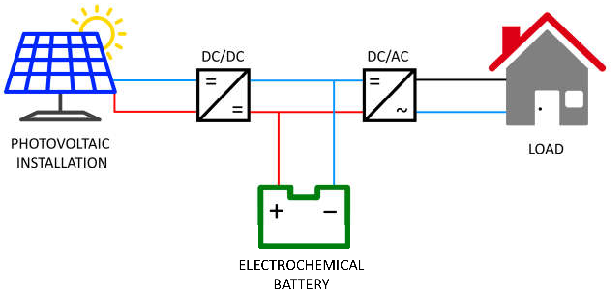
The most popular independent power supply systems with no connection to an external power grid include photovoltaic systems that work with electrochemical battery energy storage, PV/BAT. This type of system is increasingly used worldwide [7]. An illustrative scheme of an independent power generation system, consisting of a photovoltaic installation and energy storage in the form of electrochemical batteries, is shown in Figure 1.

The study of sizing a PV/BAT power generation system involves determining its configuration: the installed power of the photovoltaic installation and the rated capacity of the energy storage [8]. A wide range of methods can be used to size independent PV/BAT systems, including intuitive [9,10] and analytical [11,12] methods. In works [9,10], the authors used the intuitive method based on simple sizing equations. The input parameters were daily average values of meteorological data and load; thus, fluctuations are not considered. The results were assessed economically without analysis reliability. In turn, the analytical method uses mathematical models as a function of reliability. The calculations are simple, but the difficulty lies in the estimation coefficients of mathematical curves that are location-dependent. In work [11], the dimensioning equation was determined using a simple geometrical construction as a superposition of individual climate cycles. In this study, the economic aspects were neglected. On the other hand, in paper [12], the sizing equation was obtained using the differentiating cost function. In [11], the authors used average daily values of solar irradiation and load, while in [12], authors used monthly daily averages based on the worst month. Thus, primary energy fluctuations were not considered in both cases.

In addition, commercial software tools for optimal sizing are available. HOMER (Hybrid Optimization of Multiple Electric Renewables) was used to calculate the installed power of an independent photovoltaic system and its life cycle cost in southern Iraq [13]. HOGA (Hybrid Optimization by Genetic Algorithms) was used in [14] for sizing off-grid renewable energy systems for drip irrigation in Mediterranean crops. Simulations for residential load in Malaysia using the peak sun hour method and based on TRYNSYS (Transient System Simulation Tool) software were conducted in [15]. To assess the feasibility, based on the cost of energy, of a standalone photovoltaic system in Oman, the RETScreen program was used [16].

Attempts are also made to use artificial intelligence methods for sizing an off-grid PV/BAT power generation system [17,18]. The tabu search (TS) algorithm was used in [17] for optimal selection of the PV/BAT system configuration in smart houses in Japan. In turn, in paper [18], the sizing process of the standalone PV/BAT system was carried out with the use of a genetic algorithm (GA). This study aims at achieving an acceptable reliability level and minimum life cycle cost.

However, in the case of independent systems consisting of photovoltaic installation and electrochemical batteries, the most commonly used method is the numerical method [8,19,20]. For example, the numerical method was adopted in work [19] to develop the optimization model for the standalone PV/BAT system sizing in Algeria. After modelling components of the system and load management, the authors implemented optimization criteria based on the probability of the loss of power supply and cost of energy. The input parameters, such as meteorological variables and load demand, were adopted with an hourly time increment. For each configuration of PV installed power and rated battery capacity, the reliability indicator values were obtained. These indicators were determined using load management, as well as without it. The set of these system configurations was nominated for further analysis, which met the reliability condition based on the required probability of the loss of power supply. Then, among configurations satisfying the desired level of reliability, the optimal solution was selected based on the minimal energy cost. As research showed, the implementation of load management in the process of off-grid PB/BAT system sizing allows for a reduction in its costs. A similar approach was presented in [20], which used hourly input data based on the Malaysian meteorological profile. Within the proposed methodology, a search space was created for the installed power of PV installation and nominal battery capacity. Probability of the loss of power supply was calculated for all combinations in this search space. The best configuration was selected based on the average cost of energy from the combinations that met the desired reliability index.

The choice of the optimal sizing method applied is dictated primarily by the number of variables subject to optimization: the rated power of individual sources and the possible capacity of the energy storage. In the PV/BAT system, two parameters are optimized: the installed power of the photovoltaic installation and the storage capacity. This makes each method have a comparable degree of complexity. Expanding the structure with new electricity generation technologies, such as wind turbines, diesel generators, fuel cells, etc., increases the number of variables subject to optimization in the form of their rated power. A larger number of variables significantly hinders the use of classical methods, while methods based on artificial intelligence gain an advantage in these circumstances.

The numerical methods used for sizing independent PV/BAT systems are based on simulations, depend on energy balance calculation in each analyzed time interval, and usually consist of an hourly or daily interval. Two approaches can be adopted in these simulations: a deterministic approach that does not consider the uncertainty of the insolation data, and a probabilistic approach that considers the impact of solar variability [8]. Historical data collected over long periods can be used for the probabilistic characterization of meteorological conditions in a specific location [21]. Due to this, in the probabilistic approach, the concept of energy reliability can be used quantitatively [22].

In general, determining the optimal size of the PV installation and the battery requires the availability of the meteorological data and load demand, which makes the results highly dependent on the chosen location [23]. The authors rely on average annual values of weather variables [11] or average values of the worst month [12]. Recently, annual time series of meteorological variables have been commonly used with increments of 1 h [10].

Optimizing the HPGS structure is usually carried out by minimizing it economically while ensuring a certain level of reliability. The objective function is defined using various types of economic indicators, i.e., the cost of energy (CoE). The assumed level of reliability is ensured by adopting constraints in the algorithm, expressed by means of any reliability indicators, that is, LPSP (probability of the loss of power supply) [10,20].

The level of reliability assumed as a limitation in the sizing process is usually determined based on the initial (rated) parameters of the individual components of the analyzed power generation systems, which, in the case of PV/BAT systems, are the installed power of the photovoltaic modules and the rated capacity of the batteries [5,6,7,8,9,10,11,12,13,14,15,16,17,18,19,20,21,22,23]. This means that previously published studies on the sizing of HPGS systems do not consider the degradation of their components. Meanwhile, the decline in the efficiency of generation devices, such as photovoltaic modules or electrochemical energy converters (batteries), in the long term, affects the operational and economic indicators of the analyzed system.

In order to supplement the current state of knowledge in this area, a mathematical model was developed to size an independent power generation system consisting of a photovoltaic installation and a battery-based energy storage system, which considered long-term reliability. The authors’ first studies focused on comparing this solution with a conventional off-grid system powered by a diesel generator in terms of cost-effectiveness and environmental impact [24].

System sizing in the long-term perspective involves choosing a configuration with possibly the most beneficial value of the economic criterion indicator while meeting the reliability requirement; however, instead of setting it as the standard for the initial parameters, the reliability requirement is set for the value of the reliability indicator after years of operation, considering the decline in component performance. The result of this approach to the sizing process is oversizing of the system, i.e., selecting a configuration with a higher installed power of PV installation and rated battery capacity to ensure the desired level of reliability after years of operation. Technical oversizing of the system translates into an increase in system costs; in other words, oversizing of the system occurs from an economic perspective as well. In this article, the sizing process of the analyzed system was carried out in two ways, with and without considering the decrease in component performance. Using comparative analysis of the results of the sizing processes, the scale of oversizing (technical and economic) was determined.

In summary, the innovative nature and originality of this research lie in the model’s analysis of the operation of an independent PV/BAT system over a longer period perspective, considering degradation, and estimating the necessary scale of system oversizing in technical and economic terms. In traditional terms, the model includes a one-year analysis of the power generation system based on initial parameters without considering the decrease in performance (degradation) of the components. Therefore, this article proposes an alternative methodology for modelling and sizing the considered power generation system. The simulations were carried out using Matlab software.

2. Materials and Methods

2.1. Input Data

The model uses typical meteorological years and statistical climate data for building energy calculations, published on the Polish government’s website [25]. A Typical Meteorological Year (TMY) is a set of meteorological parameters for the entire calendar year, representing the average climate in a given geographical area. Typical meteorological years and statistical climate data for the area of Poland were compiled based on the collection of source data from the Institute of Meteorology and Water Management for 61 meteorological stations, mostly from the 30-year period between 1971 and 2000 [25]. The values of selected parameters determined for each hour of a representative calendar year were entered into the model: dry bulb temperature [°C], wind speed [m/s], and total solar radiation intensity on a surface with orientation S and inclination to the horizontal at 30° [W/m²].

The customer load profile introduced into the model was based on a standard electricity consumption profile in the distribution network of Enea Operator Sp. z o. o. (distribution network operator, Poznan, Poland) for the G11 tariff for 2021 [26]. The standard electricity consumption profile is a set of data containing the average electricity consumption in each hour of the year by a group of consumers billed in accordance with a uniform tariff plan. Standard consumption profiles are developed by distribution network operators and published in the Distribution Network Operation Instructions. Based on the standard profile of electricity consumption in the distribution network of Enea Operator Sp. z o. o. for the G11 tariff for 2021 [23], the average consumer load in the considered system in the i-th hour of the year was determined in accordance with the following formula:

$$L_i=\frac{w_i}{1000}· A_r$$

(1)

where

$L_i$—average consumer load in the considered system in the i-th hour of the year [W];

$\frac{w_i}{1000}$—relative electricity consumption in the i-th hour of the year [-];

$A_r$—annual electricity consumption by the consumer [Wh].

According to information provided by the Central Statistical Office in the report on energy consumption in households in 2018 [27], the average electricity consumption in a household was 2375 kWh. On the basis of this value of average electricity consumption, a customer load profile used in this model was prepared.

2.2. Power Generated with a PV Installation

Photovoltaic module manufacturers provide several electrical parameters in their technical documentation under STC (Standard Test Conditions) and NOCT (Normal Operating Cell Temperature) conditions. The STC correspond to a solar irradiance of 1000 W/m² and a PV module temperature of 25 °C. The NOCT conditions, on the other hand, refer to solar radiation intensity of 800 W/m², ambient temperature of 20 °C, and wind speed of 1 m/s. In both cases, the air mass factor is 1.5. Typically, PV installations are equipped with Maximum Power Point Tracker (MPPT) technology. Mathematical modelling of photovoltaic modules consists of determining the dependence of the power generated with the module on solar irradiation. It should be considered that the output power of the module also depends on its temperature. Therefore, it is necessary to determine the dependence of the temperature of the photovoltaic module on external conditions. For this purpose, the following dependencies [28] were used:

$$\frac{T_c-T_a}{T_{NOCT}-T_{a,NOCT}}=\frac{G}{G_{NOCT}}·\frac{9.5}{5.7\times 3.8·v}$$

(2)

$$T_c=\left(T_{NOCT}-T_{a,NOCT}\right)·\frac{G}{G_{NOCT}}·\frac{9.5}{5.7\times 3.8·v}+T_a$$

(3)

where

$T_c$—PV module temperature [°C];

$T_a$—ambient temperature [°C];

$T_{NOCT}$—PV module temperature in NOCT conditions [°C];

$T_{a,NOCT}$—ambient temperature in NOCT conditions [°C];

$G$—solar irradiation [W/m²];

$G_{NOCT}$—solar irradiation in NOCT conditions [W/m²];

$v$—wind speed [m/s] [28].

The power generated with the photovoltaic module can be described by the following Equation [28]:

$$P_{PV}=S·G·\left[{\eta }_{PV,STC}+\mu ·\left(T_c-T_{STC}\right)\right]$$

(4)

where

$P_{PV}$—power generated with the PV module [W];

$S$—active surface of the PV module [m²];

${\eta }_{PV,STC}$—efficiency of the PV module in STC conditions [%];

$\mu$—power temperature coefficient [%/°C];

$T_{STC}$—PV module temperature in STC conditions [°C] [28].

By inserting Equation (3) into Equation (4), the final dependence is obtained for the power generated with the photovoltaic module, and it is expressed by Equation (5).

$$P_{PV}=S·G·\left[1+\frac{\mu }{{\eta }_{PV,STC}}·\left(T_a-T_{STC}\right)+\frac{\mu }{{\eta }_{PV,STC}}·\left(\left(T_{NOCT}-T_{a,NOCT}\right)·\frac{G}{G_{NOCT}}·\frac{9.5}{5.7\times 3.8·v}\right)\right]$$

(5)

Considering that the power generated with the photovoltaic module is determined on the basis of meteorological data in a given hour of the year, Formula (5) takes the final form presented below.

$$P_i^{PV}=S·G_i·\left[1+\frac{\mu }{{\eta }_{PV,STC}}·\left(T_{a,i}-T_{STC}\right)+\frac{\mu }{{\eta }_{PV,STC}}·\left(\left(T_{NOCT}-T_{a,NOCT}\right)·\frac{G_i}{G_{NOCT}}·\frac{9.5}{5.7\times 3.8·v_i}\right)\right]$$

(6)

where

$i$—an index relating to a particular hour of the year.

The parameters of the photovoltaic module were determined on the basis of the technical documentation of an exemplary photovoltaic module with a rated power of 350 W [29]. The values of the selected parameters are listed in

Table A1. Values of selected technical parameters of the photovoltaic module adopted in the research [29].

Parameter	Symbol	Unit	Value
Active surface of the PV module	$S$	[m2]	1.5893
Power temperature coefficient	$\mu$	[%/°]	−0.36
Efficiency of the PV module in STC conditions	${\eta }_{PV,STC}$	[%]	20.51
PV module temperature in STC conditions	$T_{STC}$	[°C]	25
PV module temperature in NOCT conditions	$T_{NOCT}$	[°C]	43
Ambient temperature in NOCT conditions	$T_{a,NOCT}$	[°C]	20
Solar irradiation in NOCT conditions	$G_{NOCT}$	[W/m2]	800

, Appendix A.

2.3. Charge Level of Electrochemical Batteries

In the proposed model, the update of the energy accumulated in the battery during charging is carried out according to Equation (7):

$$C_{i+1}^{BAT}=C_i^{BAT}+{\eta }_{char}·E_i^{char}$$

(7)

and according to Equation (8), during discharging:

$$C_{i+1}^{BAT}=C_i^{BAT}-\frac{E_i^{dis}}{{\eta }_{dis}}$$

(8)

where

$C_{i+1}^{BAT}$—energy stored in the battery in the step i + 1 [Wh];

$C_i^{BAT}$—energy stored in the battery in the step i [Wh];

${\eta }_{char}$—battery charging efficiency [-];

${\eta }_{dis}$—battery discharging efficiency [-];

$E_i^{char}$—surplus energy available in the system in step i [Wh];

$E_i^{dis}$—the energy required to cover the load demand in step i [Wh] [24].

Charging and discharging takes place in the set intervals of the available battery capacity according to Equation (9):

$$C_{min}^{BAT}\le C_i^{BAT}\le C_{max}^{BAT} for i=1, \dots , n$$

(9)

where

$C_{min}^{BAT}$—the minimum assumed value of energy stored in the battery [Wh];

$C_{max}^{BAT}$—the maximum assumed value of energy stored in the battery [Wh].

If the supply or withdrawal of energy from the battery in a given simulation step results in reaching the maximum or minimum value, the update of the value of energy stored in the battery in the next step is completed according to Equations (10) and (11), respectively.

$$C_{i+1}^{BAT}=C_{max}^{BAT}$$

(10)

$$C_{i+1}^{BAT}=C_{min}^{BAT}$$

(11)

The update of the energy accumulated in the battery is preceded by a classification of the operating state the system is in. The following four operating states have been defined in which the system may be in a given simulation step:

• The power generated with the photovoltaic installation fully covers the load demand, and the battery is being charged;
• The power generated with the photovoltaic installation fully covers the load demand, and the battery is not being charged;
• The power generated with photovoltaic installation does not cover the load demand, and the battery is being discharged;
• The power generated with photovoltaic installation does not cover the load demand, and the battery is not being discharged.

The way in which to determine the energy accumulated in the battery in the next step depends on the operating state in the current simulation step.

First, the power generated with the photovoltaic installation is compared to the load demand. Both values refer to a specific hour of the year being a simulation step in the model. The condition presented by Equation (12) was formulated:

$$P_i^{PV}\ge L_i$$

(12)

where

$P_i^{PV}$—power generated with the photovoltaic installation in the i-th simulation step (i-th hour of the year) [W];

$L_i$—load demand in the i-th simulation step (i-th hour of the year) [W].

If condition of Equation (12) is met, where the power generated with the photovoltaic installation is greater than or equal to the load in the system, the load demand is covered.

The excess power in the system is determined as the difference between the power generated with the photovoltaic installation and the load demand with the use of Equation (13):

$$P_i^E=P_i^{PV}-L_i$$

(13)

where

$P_i^E$—excess power in the system in the i-th simulation step (i-th hour of the year) [W].

The excess energy in the system is determined as the product of the excess power in the system and the time corresponding to the simulation step, according to Equation (14):

$$E_i^{char}=P_i^E·\Delta t$$

(14)

where

$E_i^{char}$—excess energy in the system in the i-th simulation step [Wh];

$\Delta t$—time corresponding to the simulation step [h].

Next, it is checked whether the surplus of energy available in the system, considering the efficiency of the charging process, can be fully stored in the battery; in other words, whether charging the battery will not exceed the maximum assumed value of energy stored in the battery. This verification is carried out using the following condition of Equation (15):

$$E_i^{char}·{\eta }_{char}\le C_{max}^{BAT}-C_i^{BAT}$$

(15)

If the condition of Equation (15) is met, the update of the energy stored in the battery is completed using Equation (7). If the condition of Equation (15) is not met, it means that only a part of the surplus energy could be stored in the battery, or the charging did not take place at all due to the achievement of the maximum assumed energy value in the previous simulation steps. In such cases, the update of the energy accumulated in the battery is completed using Equation (10).

The relationships of Equations (13)–(15) apply to a situation where the power generated with a photovoltaic installation exceeds the load demand. Therefore, returning to the condition of Equation (12), the opposite case is considered below, i.e., when the load demand in the system is greater than the power generated with the photovoltaic installation.

The power deficit in the system is determined as the difference between the load demand and the power generated with the photovoltaic installation, using Equation (16):

$$P_i^D=L_i-P_i^{PV}$$

(16)

where

$P_i^D$—power deficit in the system in the i-th simulation step (i-th hour of the year) [W].

The energy required to cover the demand is determined as the product of the power deficit in the system and the time corresponding to the simulation step, according to Equation (17):

$$E_i^{dis}=P_i^D·\Delta t$$

(17)

where

$E_i^{dis}$—the energy required to cover the load demand in the i-th simulation step [Wh];

$\Delta t$—time corresponding to the simulation step [h].

Next, it is checked whether the required amount of energy, considering the efficiency of the discharge process, can be fully covered using the battery; in other words, whether the discharging of the battery will not exceed the minimum assumed value of energy stored in the battery. This verification is carried out by means of Equation (18), as follows:

$$\frac{E_i^{dis}}{{\eta }_{dis}}\le C_i^{BAT}-C_{min}^{BAT}$$

(18)

If the condition of Equation (18) is met, the update of the energy accumulated in the battery is carried out using Equation (8). However, if the condition of Equation (18) is not met, it means that only some of the required energy could be supplied from the battery, or the discharging did not occur at all due to the achievement of the minimum energy value assumed in the previous simulation steps. In such cases, the update of the energy accumulated in the battery is carried out using Equation (11).

2.4. Energy Balance in the System

In the proposed model of the PV/BAT system, the balance of covering the load demand in the system and the balance of energy generated with the photovoltaic installation were performed. The balance equations take different forms depending on the current operating state of the system. The operating states were previously defined in Section 2.3 and are defined by Equations (12), (15) and (18) in this model.

In the balance of covering the load demand in the system (Equation (19)), two energy sources (photovoltaic installation and battery) and a deficit were distinguished:

$$Z_i^{PV}+Z_i^{BAT}+Z_i^{DEF}=Z_i^{DEM}$$

(19)

where

$Z_i^{PV}$—load demand covered with the photovoltaic installation [Wh];

$Z_i^{BAT}$—load demand covered with the battery [Wh];

$Z_i^{DEF}$—energy deficit [Wh];

$Z_i^{DEM}$—load demand [Wh].

If the power generated with the photovoltaic installation is higher than or equal to the load demand ($P_i^{PV}\ge L_i$, condition of Equation (12) is met), the individual components of the balance of covering the load demand in the system take the values presented below.

$$Z_i^{PV}=L_i·\Delta t$$

(20)

$$Z_i^{BAT}=0$$

(21)

$$Z_i^{DEF}=0$$

(22)

Otherwise, when the power generated with the photovoltaic installation is lower than the load demand in the system ($P_i^{PV}<L_i$, condition of Equation (12) is not met), it is necessary to check, using Equation (18), whether it is possible to discharge the battery. If the condition of Equation (18) is met ($\frac{E_i^{dis}}{{\eta }_{dis}}\le C_i^{BAT}-C_{min}^{BAT}$), the entire energy deficit can be covered with the battery. Then, the individual components of the balance of covering the load demand in the system assume the values presented below.

$$Z_i^{PV}=P_i^{PV}·\Delta t$$

(23)

$$Z_i^{BAT}=E_i^{dis}$$

(24)

$$Z_i^{DEF}=0$$

(25)

If the condition of Equation (18) is not met ($\frac{E_i^{dis}}{{\eta }_{dis}}>C_i^{BAT}-C_{min}^{BAT}$), it means that the battery cannot be discharged ($C_i^{BAT}=C_{min}^{BAT}$) or only part of the energy required to cover the load demand can be taken from the battery. In this case, the individual components of the balance of covering the load demand in the system assume the values presented below.

$$Z_i^{PV}=P_i^{PV}·\Delta t$$

(26)

$$Z_i^{BAT}=\left(C_i^{BAT}-C_{min}^{BAT}\right)·{\eta }_{dis}$$

(27)

$$Z_i^{DEF}=L_i·\Delta t-\left(P_i^{PV}·\Delta t+\left(C_i^{BAT}-C_{min}^{BAT}\right)·{\eta }_{dis}\right)$$

(28)

In a particular case, when $C_i^{BAT}=C_{min}^{BAT}$ then

$$Z_i^{PV}=P_i^{PV}·\Delta t$$

(29)

$$Z_i^{BAT}=0$$

(30)

$$Z_i^{BAT}=0$$

(31)

In the balance of energy generated with a photovoltaic installation, the energy can be consumed in two ways in the system: by covering the load demand and charging the battery and there is also the unused energy potential of the photovoltaic installation.

$$G_i^L+G_i^{BAT}+G_i^E=G_i^{PV}$$

(32)

where

$G_i^L$—energy from the photovoltaic installation to cover the load demand [Wh];

$G_i^{BAT}$—energy from the photovoltaic installation for charging the battery [Wh];

$G_i^E$—unused energy potential of the photovoltaic installation [Wh];

$G_i^{PV}$—total energy generated with the photovoltaic installation [Wh].

If the power generated with the photovoltaic installation is higher than or equal to the load demand ($P_i^{PV}\ge L_i$, condition of Equation (12) is met), it is necessary to check, using Equation (15), whether it is possible to charge the battery. If the condition of Equation (15) is met ($E_i^{char}·{\eta }_{char}\le C_{max}^{BAT}-C_i^{BAT}$), it means that all surplus energy can be stored in the battery. Therefore, the individual components of the balance of energy generated with the PV installation assume the values presented below.

$$G_i^L=L_i·\Delta t$$

(33)

$$G_i^{BAT}=E_i^{char}$$

(34)

$$G_i^E=0$$

(35)

If the condition of Equation (15) is not met ($E_i^{char}·{\eta }_{char}>C_{max}^{BAT}-C_i^{BAT}$), it means that the battery cannot be charged ($C_i^{BAT}=C_{max}^{BAT}$) or only part of the surplus energy can be stored there. In this case, the individual components of the balance of energy generated with the PV installation take the values presented below.

$$G_i^L=L_i·\Delta t$$

(36)

$$G_i^{BAT}=\frac{\left(C_{max}^{BAT}-C_i^{BAT}\right)}{{\eta }_{char}}$$

(37)

$$G_i^E=E_i^{char}-\frac{\left(C_{max}^{BAT}-C_i^{BAT}\right)}{{\eta }_{char}}$$

(38)

In a particular case, when $C_i^{BAT}=C_{max}^{BAT}$ then

$$G_i^L=L_i·\Delta t$$

(39)

$$G_i^{BAT}=0$$

(40)

$$G_i^E=E_i^{char}$$

(41)

When the power generated with the photovoltaic installation is lower than the load demand in the system ($P_i^{PV}<L_i$, condition of Equation (12) is not met), the individual components of the balance of energy generated with the PV installation take the values presented below.

$$G_i^L=P_i^{PV}·\Delta t$$

(42)

$$G_i^{BAT}=0$$

(43)

$$G_i^E=0$$

(44)

2.5. Degradation of System Components

Modelling the impact of degradation on the operation of the PV/BAT system components is understood as a way to update the parameters determining the performance of power equipment. Both photovoltaic modules and electrochemical batteries are subject to degradation processes.

In the case of photovoltaic modules, a parameter directly related to energy performance is the available output power. Due to the decrease in the efficiency of photovoltaic modules, with the same solar irradiation value, less and less output power will be obtained over time. Based on a review of the technical specifications of the PV modules available on the market, it can be concluded that the efficiency related to the rated power is between 97% and 98% in the first year, with a loss of 0.3% to 1.0% per year in subsequent years of operation [30]. The model assumes a degradation rate of 2.5% during the first year and a further annual decrease in performance of 1% in relation to the rated power.

The degradation process of electrochemical batteries was modelled using the loss of capacity and the decrease in the charging and discharging efficiency resulting from the increase in the internal resistance of the cells. The decrease in charging and discharging efficiency was assumed on the basis of operational experience as a value of 1% per year, with 99% being the initial value, which is achievable for lithium-ion cells [31]. On the other hand, the loss of capacity depended on the number of batter charge and discharge cycles.

The rate of capacity loss along with the number of cycles is related to the nature of battery operation, and more specifically, to the capacity range in which the charging and discharging process takes place. This range is defined in this model with the minimum and maximum value of energy stored in the battery (capacity)—$C_{min}^{BAT}$ and $C_{max}^{BAT}$.

In this model, the relationship describing the loss of battery capacity depending on the number of work cycles is implemented, as presented in [32], for the range of utilized capacity between 25% and 100%. The selected waveform was approximated and implemented in this model for the annual update of the available battery capacity. For the best mapping, the literature-based waveform was approximated partly by a quadratic function and partly by a linear function:

$$C=\left\{\begin{array}{c}8\times {10}^{-6}\times l_C{}^2-0.017\times l_C+99.804 dla l_C<900\\ -0.0033\times l_C+93.923 dla l_C\ge 900\end{array}\right.$$

(45)

where

$C$—available battery capacity [%];

$l_C$—number of battery work cycles [-].

To count the number of cycles, the rainflow counting algorithm was used. This method was originally used in the field of strength mechanics to analyze the progress of the degradation process in cyclic operation. More recently, it has also been widely used to count the working cycles of electrochemical batteries [33].

2.6. Solution Evaluation Parameters

In this model, two indicators were used to evaluate the solutions, the reliability indicator and the economic indicator.

To evaluate the solutions in terms of energy reliability, the Loss of Load Probability (LOLP) indicator was used. The LOLP indicator is a measure of the probability that the demand for power will exceed the power generation capacity of the system in a given period of time [34]. The LOLP indicator is calculated according to formula (46):

$$LOLP=\frac{{{\displaystyle \sum }}_{i=1}^n{E}_i^{DNC}}{{{\displaystyle \sum }}_{i=1}^n{E}_i^D}·100\%$$

(46)

where

$E_i^{DNC}$—electricity deficit in the system in the i-th simulation step [kWh];

$E_i^D$—demand for electricity in the system in the i-th simulation step [kWh].

To evaluate the solutions from an economic point of view, the Levelized Cost of Electricity (LCOE) indicator was used. The LCOE indicator is used to determine the unit cost of electricity production in the system. This indicator is determined as the ratio of the total costs of the system to the value of energy produced by the system over the entire period of operation. The LCOE is a commonly used measure to compare different power systems from an economic point of view. It is described by Equation (47):

$$LCOE=\frac{I_0+{{\displaystyle \sum }}_{t=1}^m\frac{K_t}{{\left(1+r\right)}^t}}{{{\displaystyle \sum }}_{t=1}^m\frac{\left(E_i^D-E_i^{DNC}\right)}{{\left(1+r\right)}^t}}$$

(47)

where

$I_0$—capital expenditures;

$K_t$—total annual costs;

$r$—discount rate;

$t$—year of operation;

$m$—years of operation in the analyzed period.

Using the cost index CAPEX (Capital Expenditures)—referring to investment outlays—and OPEX (Operational Expenditures)—referring to the costs of maintenance and operation—in the field of renewable energy sources, Equation (47) can be presented in the form (48):

$$\begin{gathered} LCOE=\frac{CAPEX+{{\displaystyle \sum }}_{t=1}^m\frac{OPE{X}_t}{{\left(1+r\right)}^t}}{{{\displaystyle \sum }}_{t=1}^m\frac{\left(E_i^D-E_i^{DNC}\right)}{{\left(1+r\right)}^t}} \\ =\frac{{CAPEX}^{PV}{+CAPEX}^{BAT}+{{\displaystyle \sum }}_{t=1}^m\frac{{OPEX}_t^{PV}+{OPEX}_t^{BAT}}{{\left(1+r\right)}^t}}{{{\displaystyle \sum }}_{t=1}^m\frac{\left(E_i^D-E_i^{DNC}\right)}{{\left(1+r\right)}^t}} \end{gathered}$$

(48)

where

$CAPE{X}^{PV}$—capital expenditures for PV installation;

$CAPE{X}^{BAT}$—capital expenditures for lithium-ion electrochemical batteries;

${OPEX}^{PV}$—operational expenditures for PV installation;

${OPEX}^{BAT}$—operational expenditures for lithium-ion electrochemical batteries.

The adopted economic parameters are listed in

Table A2. Values of selected economic parameters adopted in the research.

Parameter	Symbol	Unit	Value
Unit capital expenditures for PV installation [35]	$CAPE{X}_u^{PV}$	$[\mathrm{EUR} /{\mathrm{kW}}_{\mathrm{p}}]$	460
Unit capital expenditures for lithium-ion electrochemical batteries [35]	$CAPE{X}_u^{BAT}$	$\left[\mathrm{EUR} /\mathrm{kWh}\right]$	275
Unit operational expenditures for PV installation [35]	$OPE{X}_u^{PV}$	$[\mathrm{EUR} /{\mathrm{kW}}_{\mathrm{p}}/\mathrm{year}]$	9.2
Unit operational expenditures for lithium-ion electrochemical batteries [35]	$OPE{X}_u^{BAT}$	$\left[\mathrm{EUR} /\mathrm{kWh}/\mathrm{year}\right]$	4.1
Discount rate	$r$	[%]	7

, Appendix B.

2.7. Simulation Process

The mathematical model for sizing the PV/BAT power generation system presented in Section 2.1–Section 2.6, considering the degradation of elements, allowed us to carry out exemplary simulations to assess its effectiveness.

The simulation process is initiated by loading the input data, which mainly includes meteorological data and the load profile (Section 2.1). In addition, the search space is defined at the initial stage, related to the sizing of the system.

The sizing of the considered system is a task that outlines the selection of the best solution, in accordance with the adopted criteria, which depends on two variables: the power of the photovoltaic installation and the capacity of the electrochemical battery. Thus, the range and step are determined for the above-mentioned variables with which the simulations are performed. As a result, a two-dimensional search space is created in this model. The adopted range and step of the variables were adapted to the scope of research presented in this article; however, due to the versatility of the model, simulations can be performed for any search space. For the purposes of this article, the power of the photovoltaic installation was changed in from 0.7 kW_p to 50.5 kW_p in increments of 0.7 kW_p, while the energy storage capacity was changed in from 2.5 kWh to 60 kWh in increments of 2.5 kWh.

After loading the input data, simulations of the first year of system operation are performed. For each variant of the system design (in line with the adopted search space), iteratively for each hour of the year, a current update of the battery charge status is performed (Section 2.3) and energy balances are carried out (Section 2.4). Simulations of a full year of operation make it possible to determine the waveforms of key quantities, i.e., the power deficit and the value of energy stored in the battery. Based on the waveform of the power deficit in the system, the annual LOLP indicator is determined (Section 2.6), while the waveform of energy accumulated in the battery allows to determine the number of charging and discharging cycles (Section 2.5).

The results of the annual analysis are saved, and the procedure is repeated for subsequent years of system operation, but the parameters that determine the performance of system components and change the value as a result of degradation are subject to updating (Section 2.5). A 15-year period of system operation was analyzed.

The LOLP indicator (Section 2.6) was determined for each year of operation. On the other hand, the LCOE index (Section 2.6), by definition, covers the entire service life. It has been determined in two ways. The first method of calculating the LCOE indicator does not consider the degradation process, i.e., it was assumed that throughout its lifetime the system operates as it did in year one. The second method of calculating the LCOE considers the degradation process, i.e., the systems’ energy production data changes in subsequent years. The results were subjected to comparative analysis.

The selection of the best variant of the system configuration from the search space is made on the basis of the lowest value of the LCOE indicator among the combinations that do not exceed the set value of the LOLP indicator. In other words, the best solution is selected on the basis of the economic criterion, while satisfying the reliability condition. The LCOE is the minimized objective function and LOLP is the constraint. As a reliability constraint, a condition was adopted that in the last 15th year of operation, the LOLP indicator would not exceed 5%, as shown below.

$$\mathrm{LCOE} \to \min \bigwedge { \mathrm{LOLP}}_{t=15}\le 5\%$$

(49)

The choice of the best system configuration in the adopted search space was made without considering the decrease in component performance and with its inclusion for the selected capacity range in which the battery charging and discharging process occurs (Section 2.5).

3. Results

This section presents the simulation results of the long-term operation of an independent photovoltaic system with electrochemical energy storage, whose charging and discharging took place within the permissible range of 25–100% of the available capacity. Simulations were carried out for all configurations of the installed power of photovoltaic modules ($P_{nom}^{PV}$) and the rated storage capacity ($C_{nom}^{BAT}$) from the search space analyzed (Section 2.7). The simulation culminates in finding the system configuration that hast the highest cost effectiveness when the reliability condition is met.

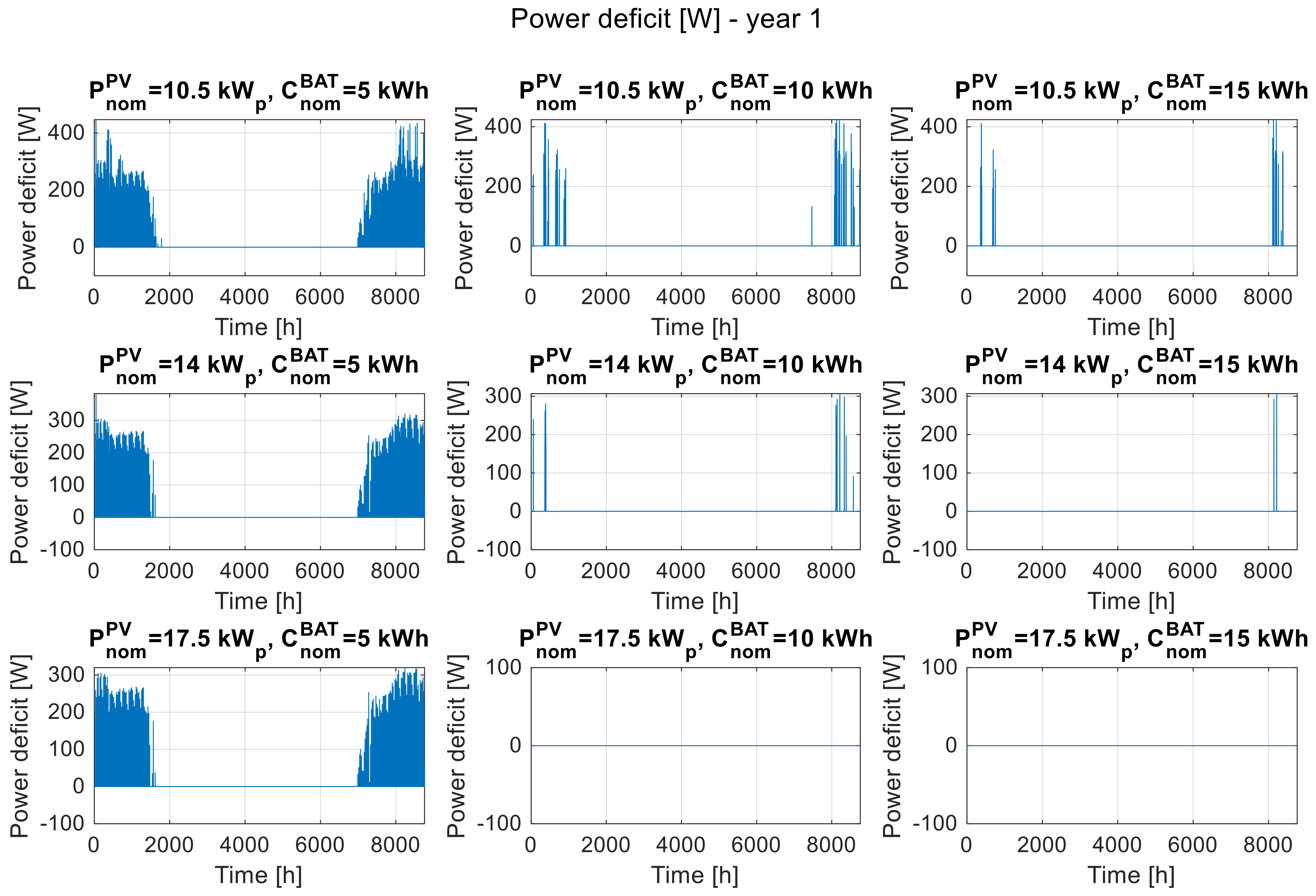
3.1. Power Deficit

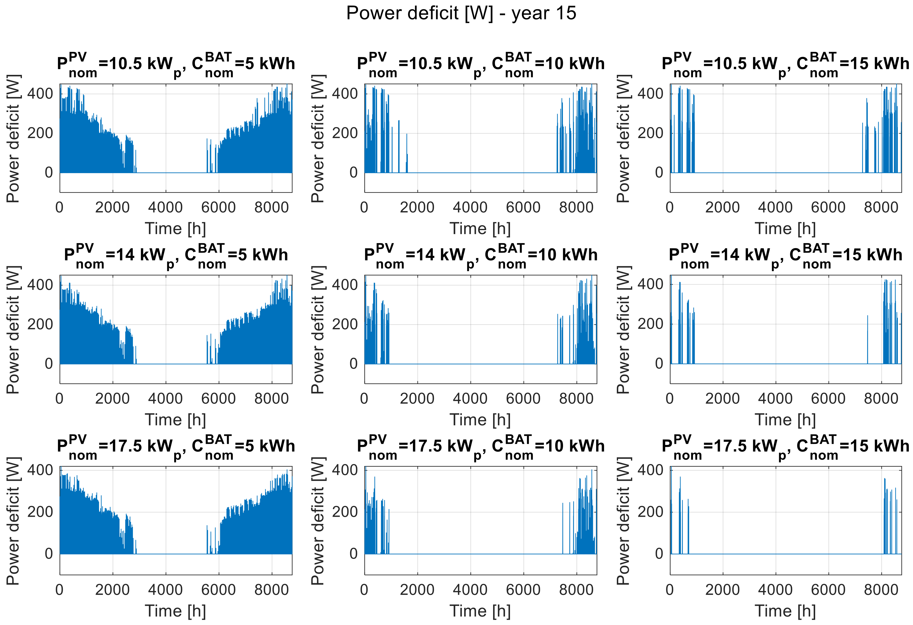
Figure 2, Figure 3 and Figure 4 show the waveform of the power deficit in the system in each hour of the first, eighth, and last year of operation and include nine selected system configurations, for the installed PV power of 10.5 kW_p, 14 kW_p, and 17.5 kW_p and for the nominal storage capacity of 5 kWh, 10 kWh, and 15 kWh. All graphs, for the first, eighth, and last year of operation, show that the power deficit occurs mainly in the winter. The zero-power deficit in the summer means that the system is able to fully cover the load demand of the recipient.

The juxtaposition of nine configurations of the system structure shows that increasing the installed PV power and/or nominal battery capacity allows to reduce or eliminate the expected power deficit, while the effects are more noticeable in the case of oversized storage. By comparing the corresponding waveforms of the power deficit in Figure 2, Figure 3 and Figure 4, the impact of the degradation of the system components on its power generation performance can be seen, manifested by the growth of the power deficit over the years of operation. The power deficit in the 8th and 15th year of operation is observed in winter in configurations for which it did not occur in the initial period of operation.

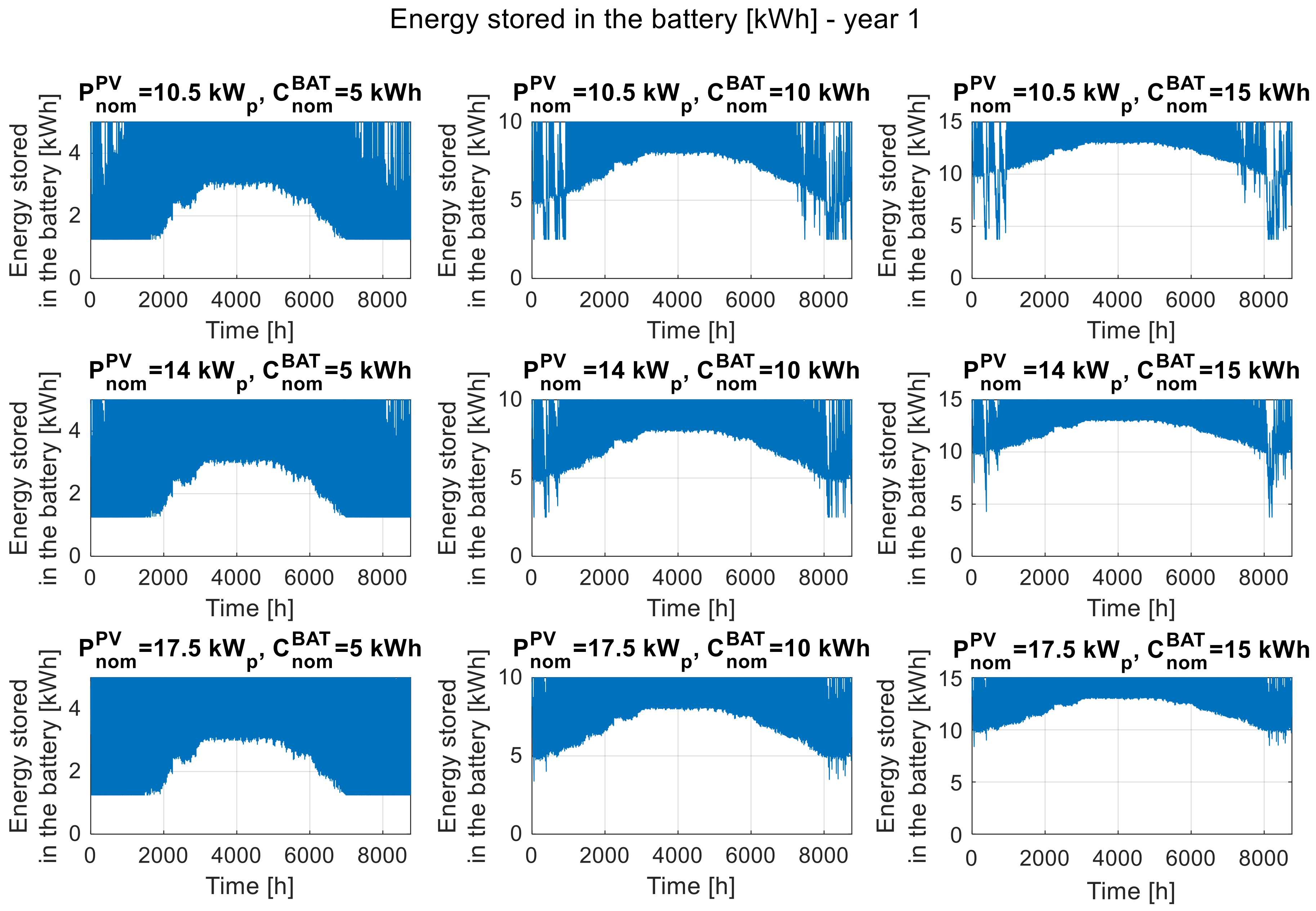
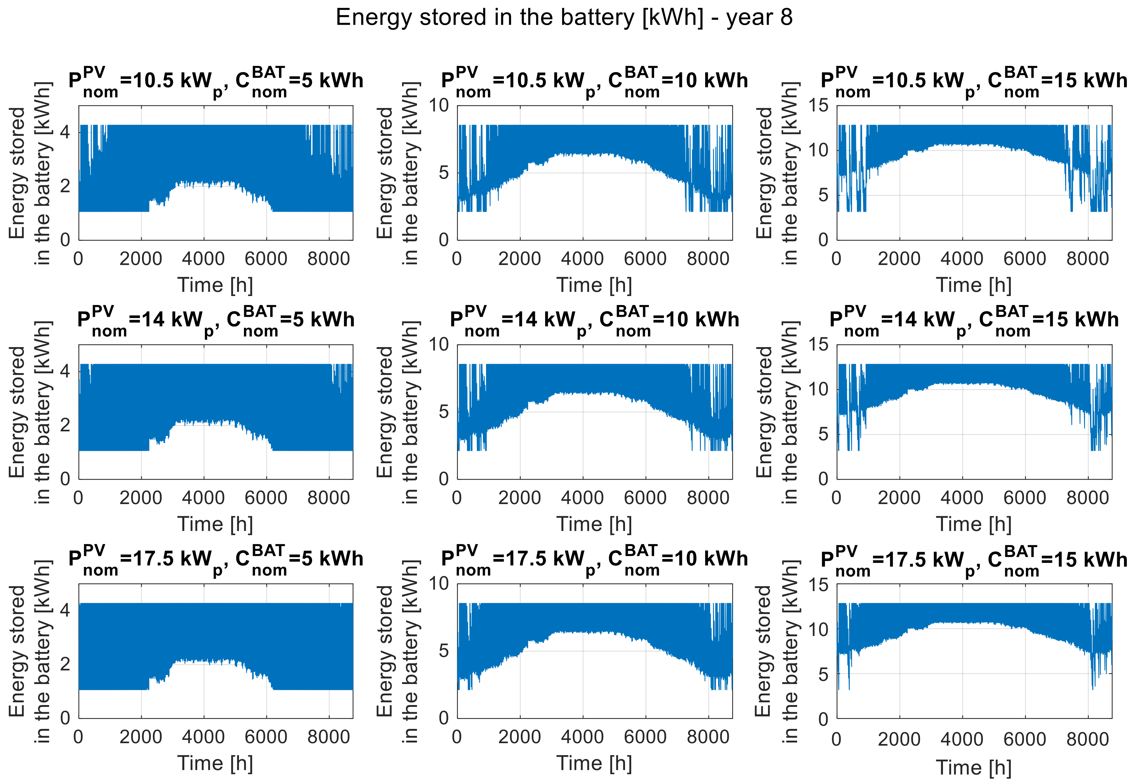
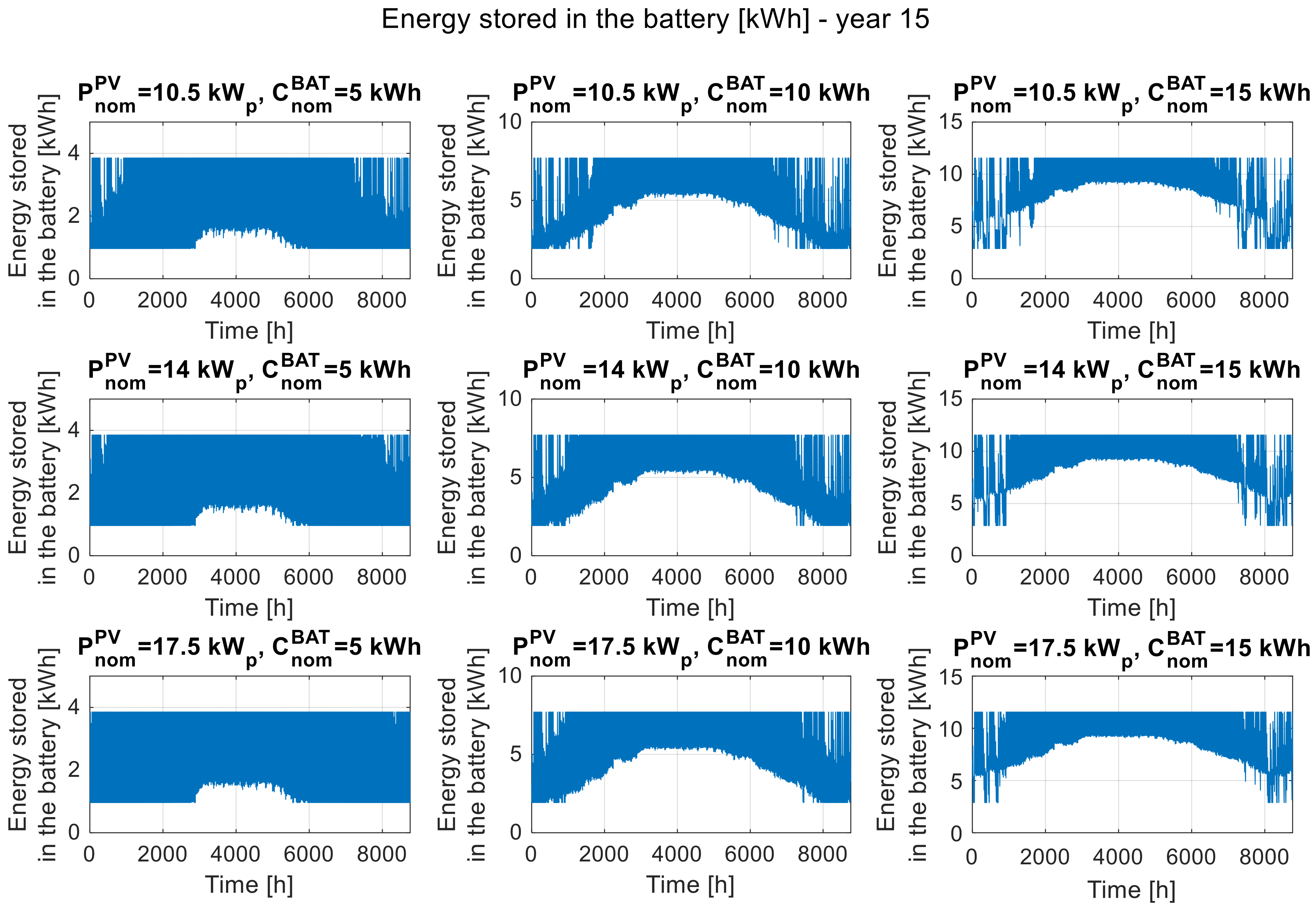
3.2. Energy Stored in the Battery

Figure 5, Figure 6 and Figure 7 show the waveforms of energy stored in the battery at each hour of the first, eighth, and last year of operation for the same selected system configurations as the power deficit waveforms (Figure 2, Figure 3 and Figure 4). The lower the battery capacity, the greater its usage range (in terms of percentage), i.e., the battery is discharged to the minimum assumed level more often. Increasing the battery capacity causes it to be discharged in a smaller capacity range (in terms of percentage). This effect is observed in the summer season, and with increasing nominal value of battery capacity, it expands for the winter period. A similar effect causes an increase in installed photovoltaic power, but in this case, the effect is less visible (only in winter) and occurs less frequently. By comparing the corresponding waveforms of energy stored in the battery shown in Figure 5, Figure 6 and Figure 7, the effect of degradation on the available storage capacity and the more frequent use of energy stored in the battery, due to a decrease in the performance of the PV modules, can be observed.

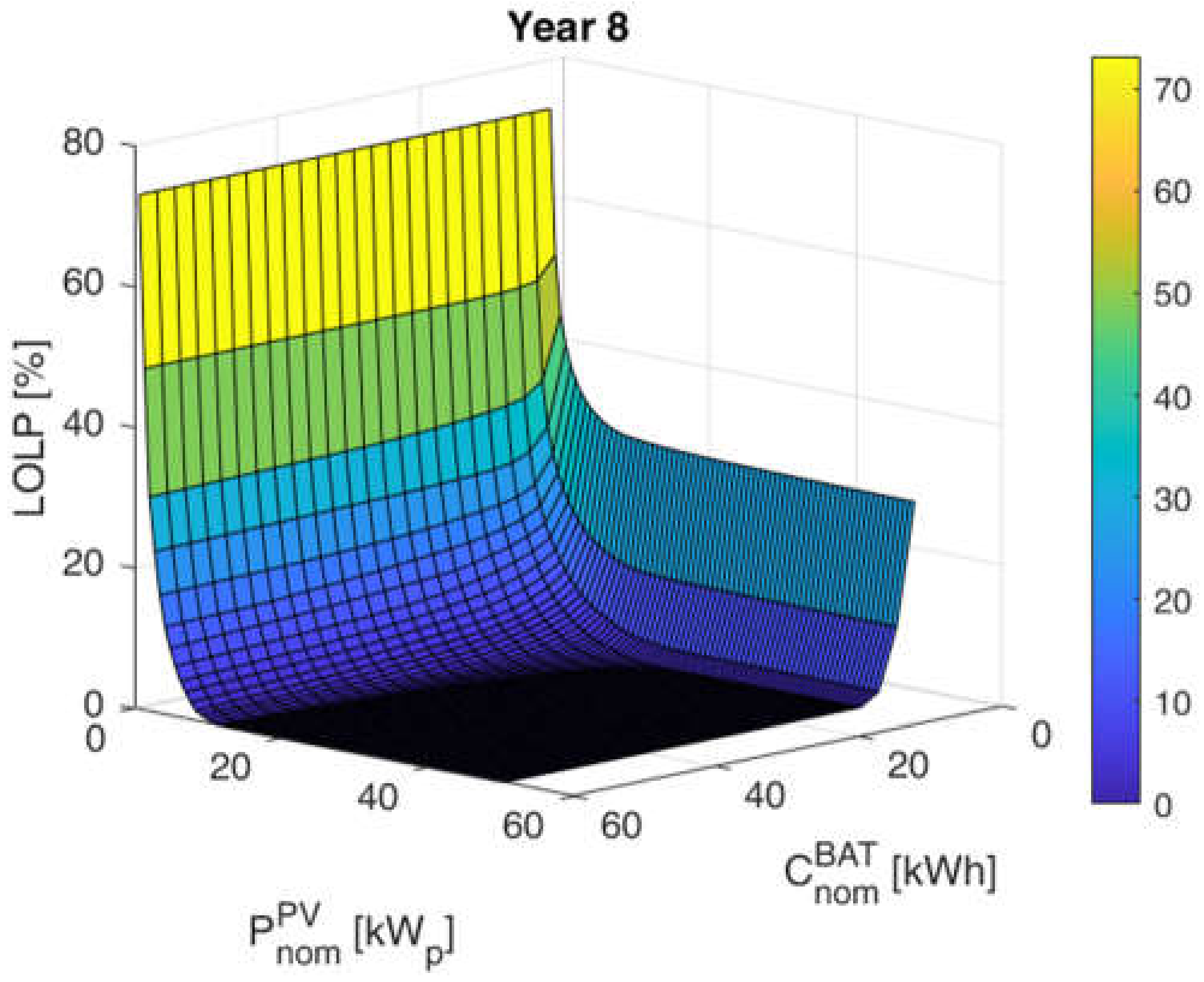
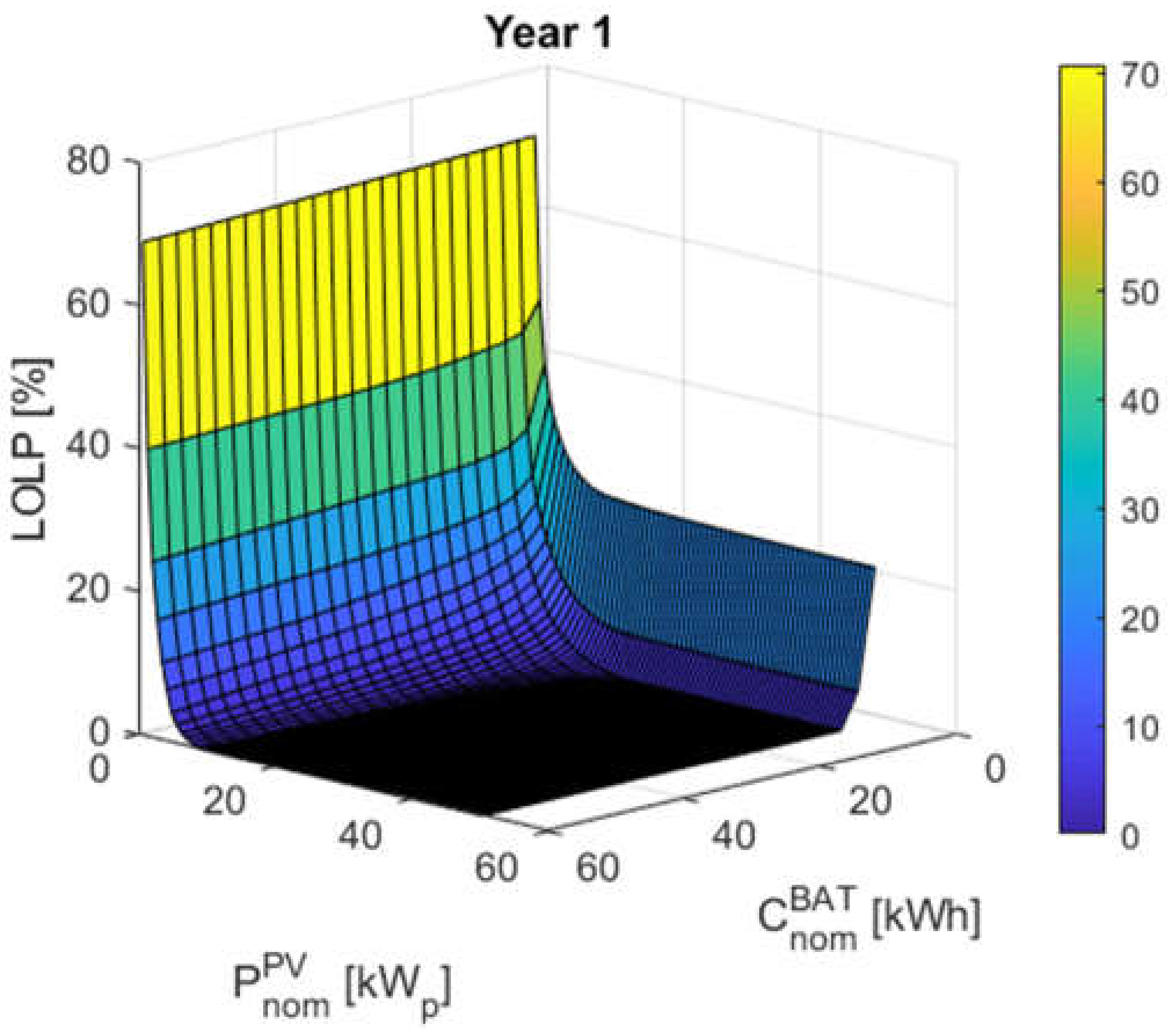
3.3. LOLP Reliability Indicator

The determined power deficit waveforms allow for the calculation of the total energy deficit in a given year. On this basis, the LOLP indicator was determined for each system configuration from the search space, and the results are presented in Figure 8, Figure 9 and Figure 10 for the first, eight, and fifteenth year of operation, respectively.

Comparing the graphs of the LOLP function ($LOLP=f\left(P_{nom}^{PV}, C_{nom}^{BAT}\right)$) for the first, eighth, and last year of operation (Figure 8, Figure 9 and Figure 10), it can be observed that its values are higher for the fifteenth year of operation in the case of a significant part of the considered configurations. A higher value of the LOLP indicator means a higher probability of failure to cover the load demand in the considered system. Even if a given variant of the PV/BAT system meets the required level of reliability in the first year of operation, it may exceed its permissible value in the following years of operation due to the progressive degradation processes and the decreased performance of the system’s components. The situation of an increase in the LOLP indicator during the years of operation applies to configurations with values from the beginning of the considered ranges of the installed power of the photovoltaic installation and the nominal storage capacity. Some of the results of the system configuration provide the desired or even a zero LOLP level, which is associated with the appropriate oversizing of the system.

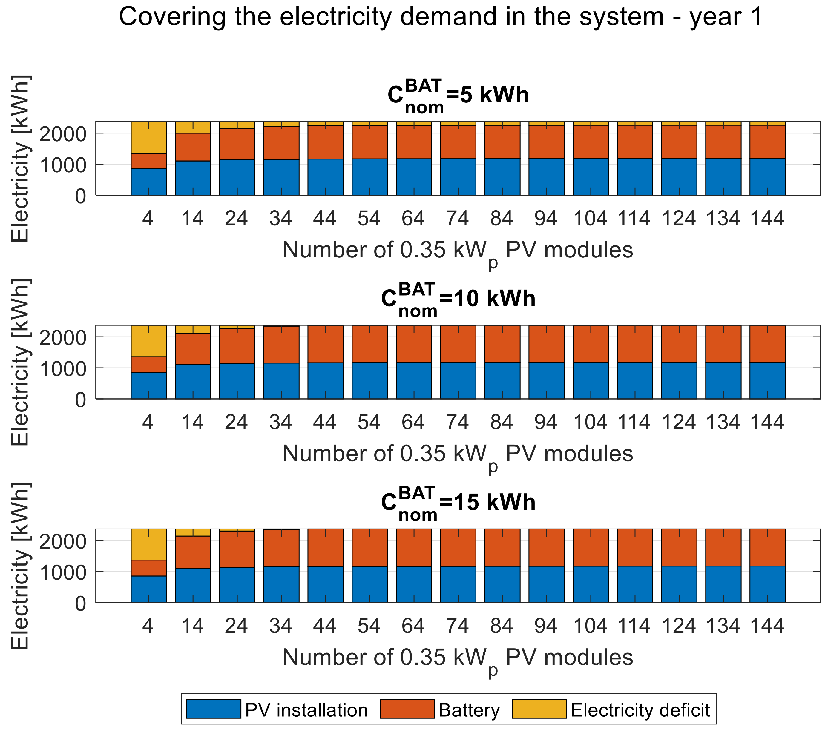
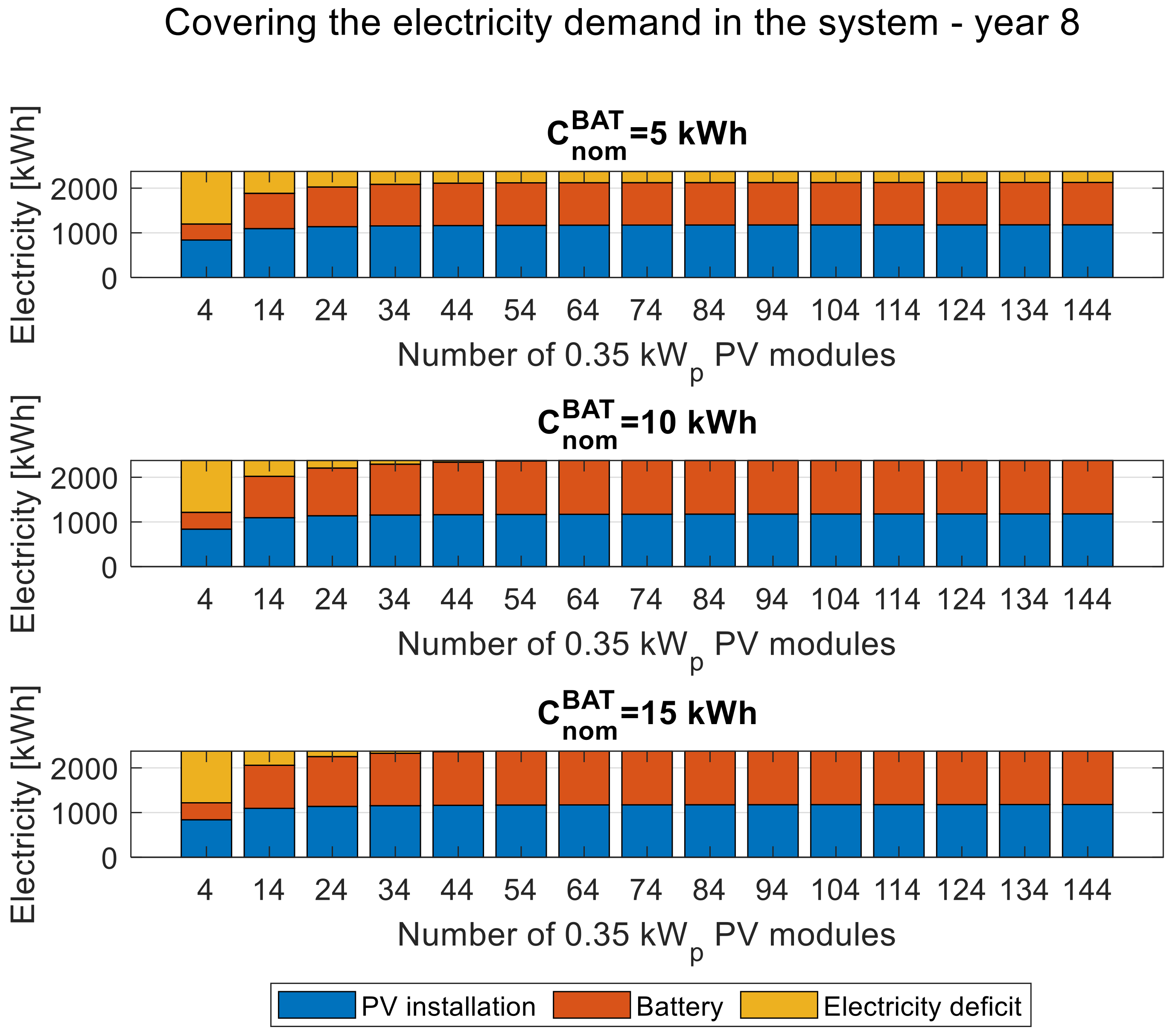
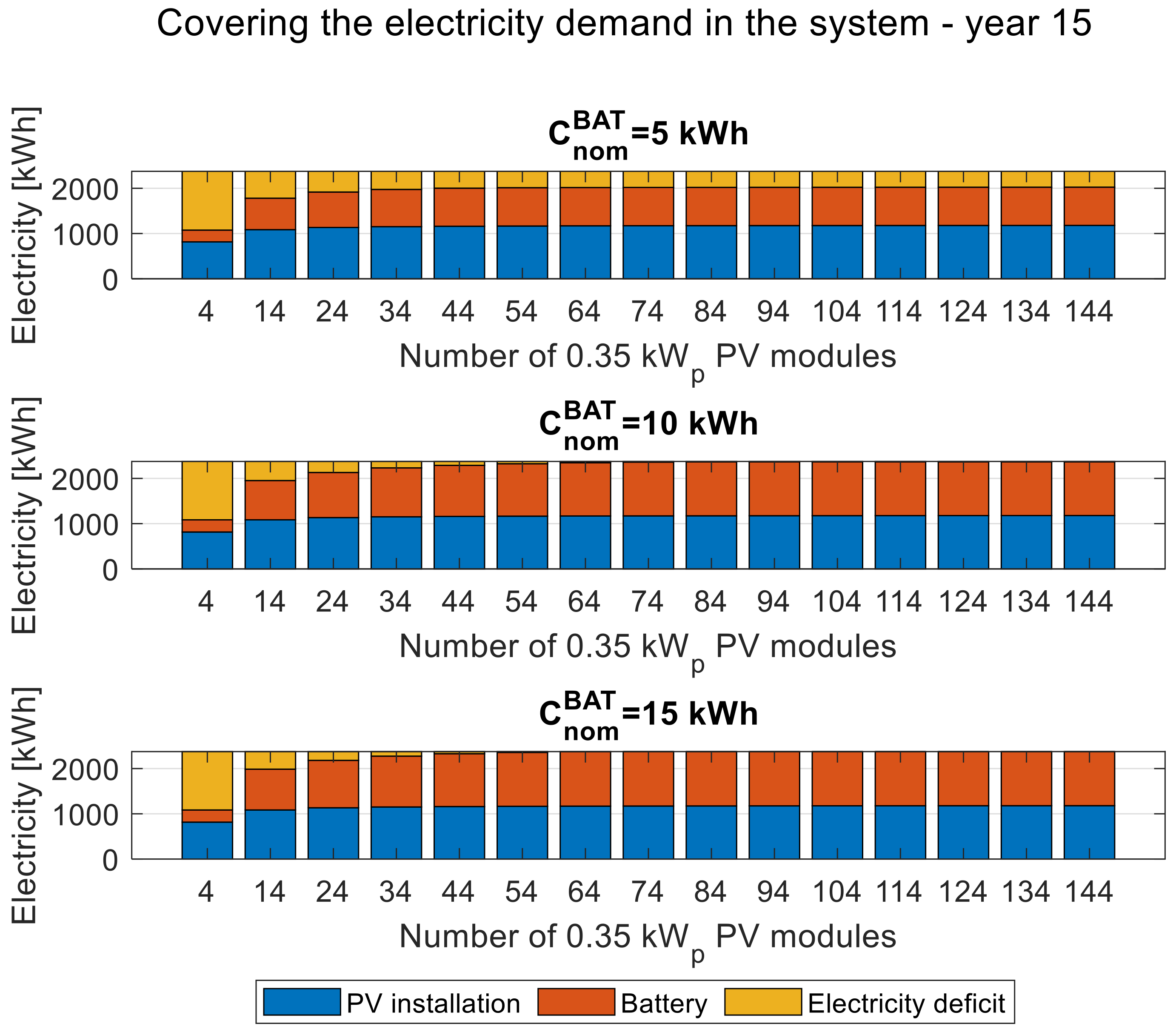
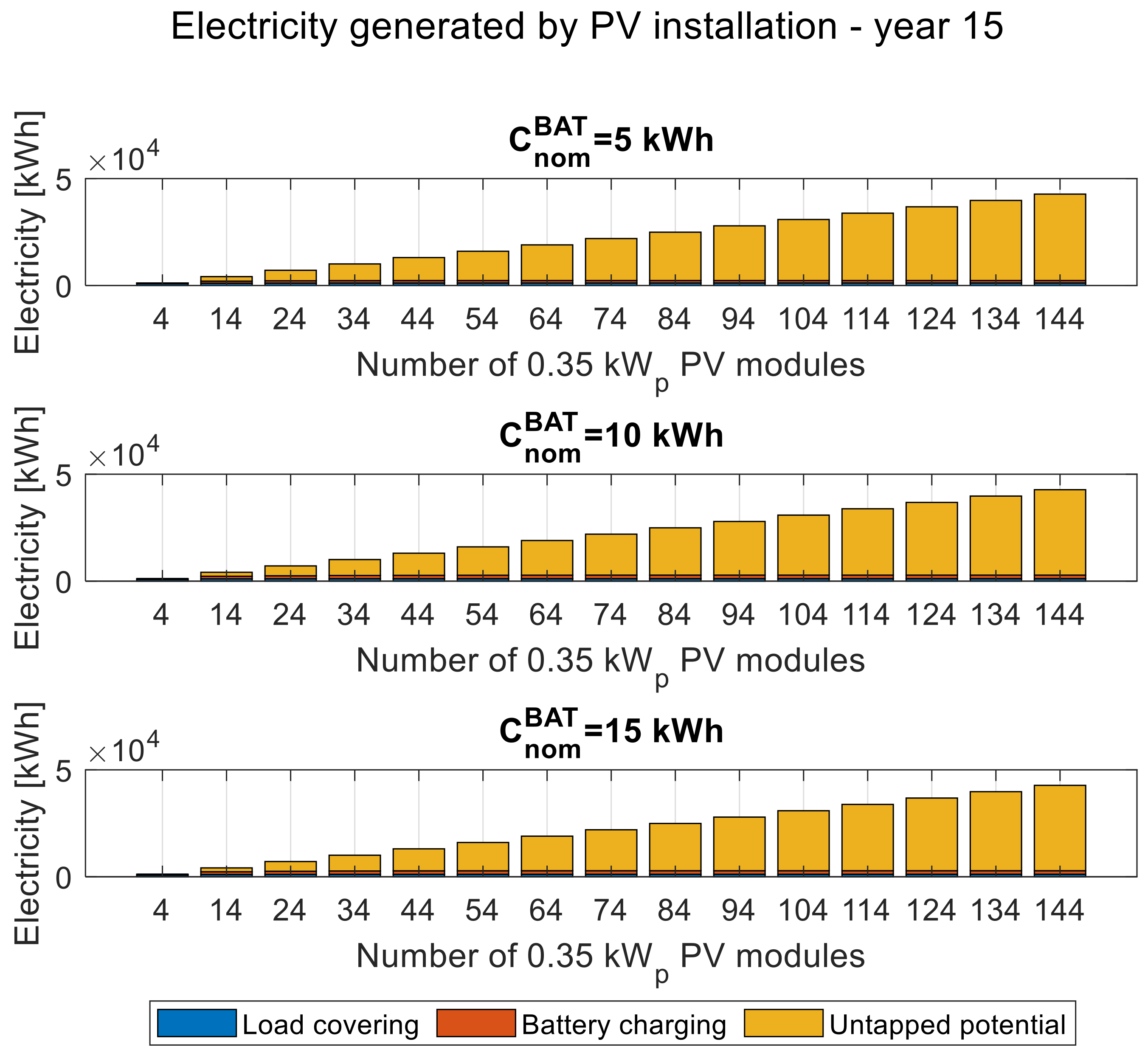
3.4. Energy Balances

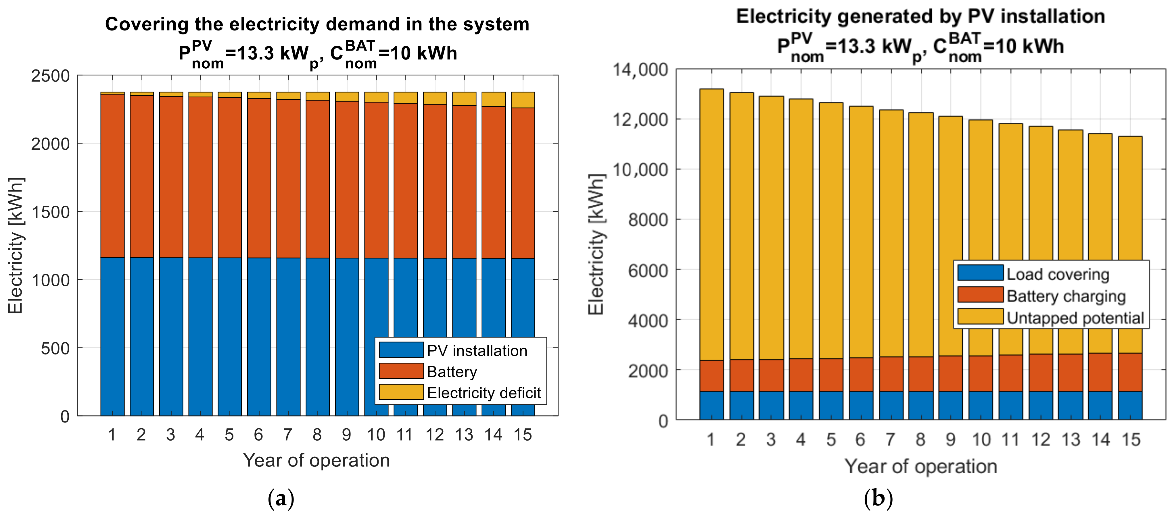
Figure 11, Figure 12, Figure 13, Figure 14, Figure 15 and Figure 16 show a graphical presentation of the energy balances performed during the simulation. Figure 11, Figure 12 and Figure 13 present the balance of covering the load demand in the system, while Figure 14, Figure 15 and Figure 16 present the balance of energy generated with the photovoltaic installation. Both balances are presented in the first, eighth, and last year of operation, respectively. The balances for the three selected variants of the nominal battery capacity, 5, 10, and 15 kWh, are presented in the form of bar graphs depending on the increasing number of PV modules, which can be easily translated into the installed power of the PV installation.

When analyzing the balance of covering the load demand in the system, it can be noticed that the higher the storage capacity is, the smaller the number of PV modules required to eliminate the energy deficit in the system are. However, if the battery capacity is too small for the considered system (5 kWh), even a further increase in the installed power of the PV installation will not eliminate the energy deficit. When comparing the corresponding balances of covering the load demand in the system in the first (Figure 11), eighth (Figure 12), and the last (Figure 13) year of operation, it is observed that for the selected storage capacity, the complete elimination of the energy deficit in the fifteenth year requires about double the installed PV capacity compared to the first year.

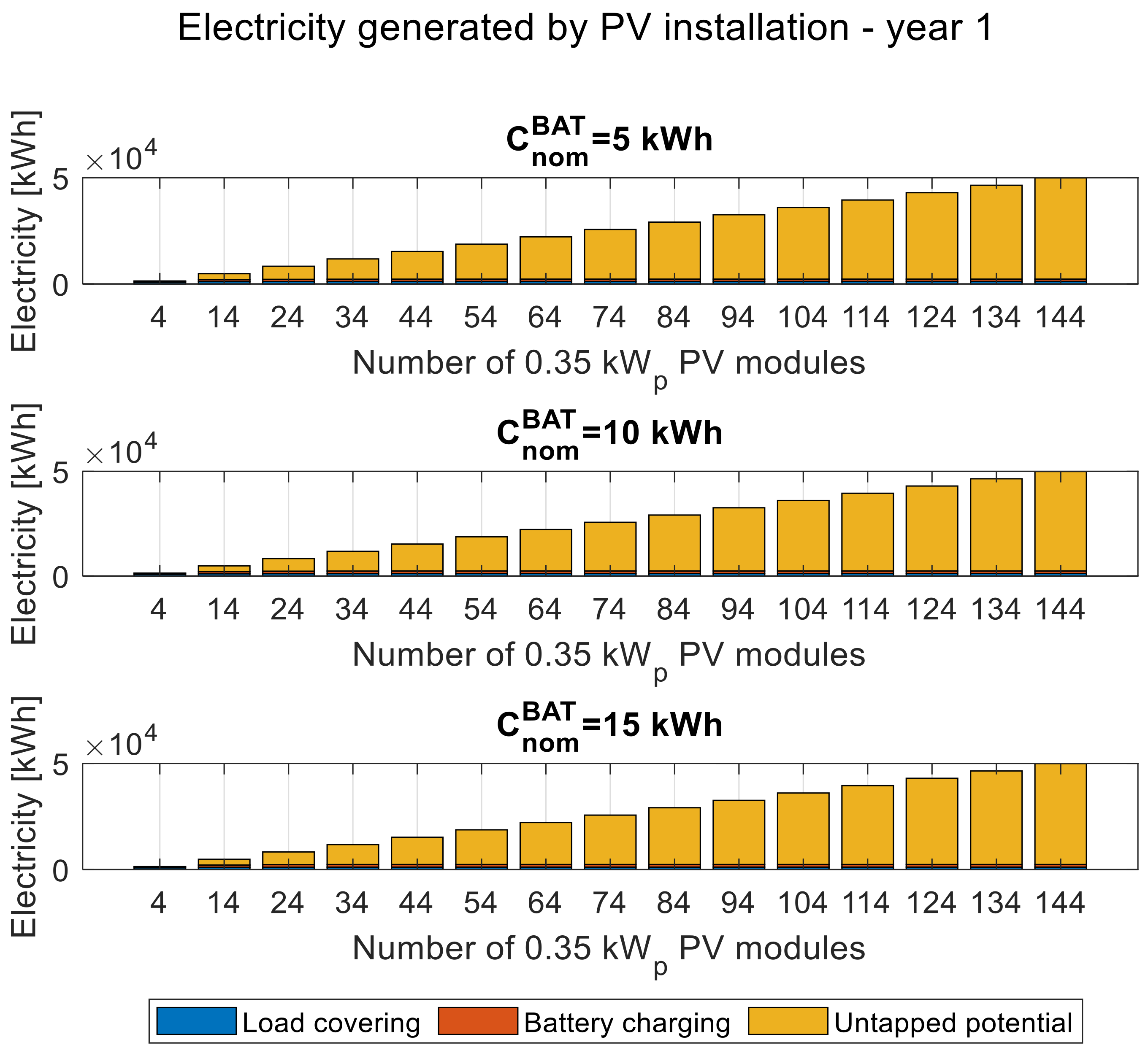
The balances of energy generated with the photovoltaic installation in the first (Figure 14), eighth (Figure 15), and last (Figure 16) year of operation show the increasing share of energy allocated to covering the load demand and charging the battery, as well as the scale of possible oversizing to ensure long-term reliability.

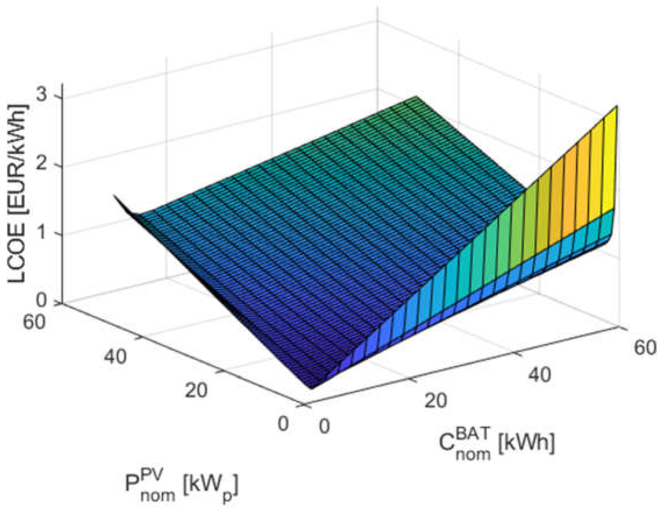
3.5. LCOE Economic Indicator

The final stage of the PV/BAT system sizing process, following the simulations for all years of operation, is the calculation of the economic performance using the LCOE indicator that expresses the cost of electricity generation in the system. The LCOE indicator that calculated for all system configurations in the search space assumes a 15-year system operation. The total energy produced and consumed by the system during this period varies depending on whether degradation of the components is considered. Therefore, the LCOE indicator can be determined in two ways, including and excluding the decrease in system performance. The values of the LCOE indicator determined based on 15 years of operation, while considering the degradation depending on the nominal battery capacity and the installed power of the photovoltaic installation, are shown in the graph in Figure 17. The graph of the function $\mathrm{LCOE}=f\left(P_{nom}^{PV}, C_{nom}^{BAT}\right)$ is determined when the decrease in the performance of the system components is ignored and is analogous, but the values of the LCOE indicator are lower for the corresponding configurations. This follows directly from Equation (48).

3.6. Selection of the Optimal Configuration of the PV/BAT System

The completed simulations of the operation of the PV/BAT system, and the determination of the reliability (LOLP) and economic (LCOE) indicators, made it possible to determine the best system configuration from the point of view of the adopted criteria. The best solution from the search space is the configuration with the lowest LCOE among the configurations that guaranteed the value of the LOLP indicator below the assumed level of 5% in the 15th year of operation. The results of the sizing process are different when degradation is considered and when it is not. If degradation is neglected, it can be assumed that the LOLP is the same in both the first and last year of operation. If component degradation is considered, the LOLP indicator is, according to the simulations, higher in the last year of operation than in the first year. This eliminates part of the configurations due to the failure to meet the reliability condition.

Table 1. The results of the sizing process, considering and not considering the degradation of the elements of the given system, for charging and discharging the battery in the range of 25–100% of the available capacity.

	Degradation Considered	Degradation Not Considered
Nominal battery capacity $C_{nom}^{BAT}$ [kWh]	7.5	10
Installed power of PV installation $P_{nom}^{PV}$ [kWp]	11.2	13.3
LOLP reliability indicator in 15th year of operation LOLPt=15 [%]	4.9097	4.8853
LCOE economic indicator [EUR/kWh]	0.4100	0.4899

shows the results of the sizing process, considering and not considering the degradation of the elements of the given system, in the case of charging and discharging the battery in the range of 25–100% of the available capacity.

When neglecting component degradation and, at the same time, meeting the reliability criterion, the lowest LCOE value was obtained for the nominal battery capacity equal to 7.5 kWh and the installed power of the photovoltaic installation equal to 11.2 kW_p. This configuration provides an LCOE of EUR 0.41/kWh.

Considering the degradation of the components, the previously selected system configuration (7.5 kWh, 11.2 kW_p) is unable to provide the required level of reliability in the 15th year of operation (LOLP ≤ 5%). To achieve the desired level of reliability in the last year of operation, it is necessary to oversize the system. In this case, the lowest LCOE value was achieved, while ensuring the required LOLP value, for the nominal battery capacity of 10 kWh and the installed power of the photovoltaic installation of 13.3 kW_p. This configuration provides an LCOE of EUR 0.4899/kWh.

Taking degradation into account in the sizing process resulted in an increase in the nominal capacity of the battery by 33.33%, an increase in the installed power of the photovoltaic installation by 18.75%, and an increase in the cost of electricity in the system (LCOE) by 19.5%.

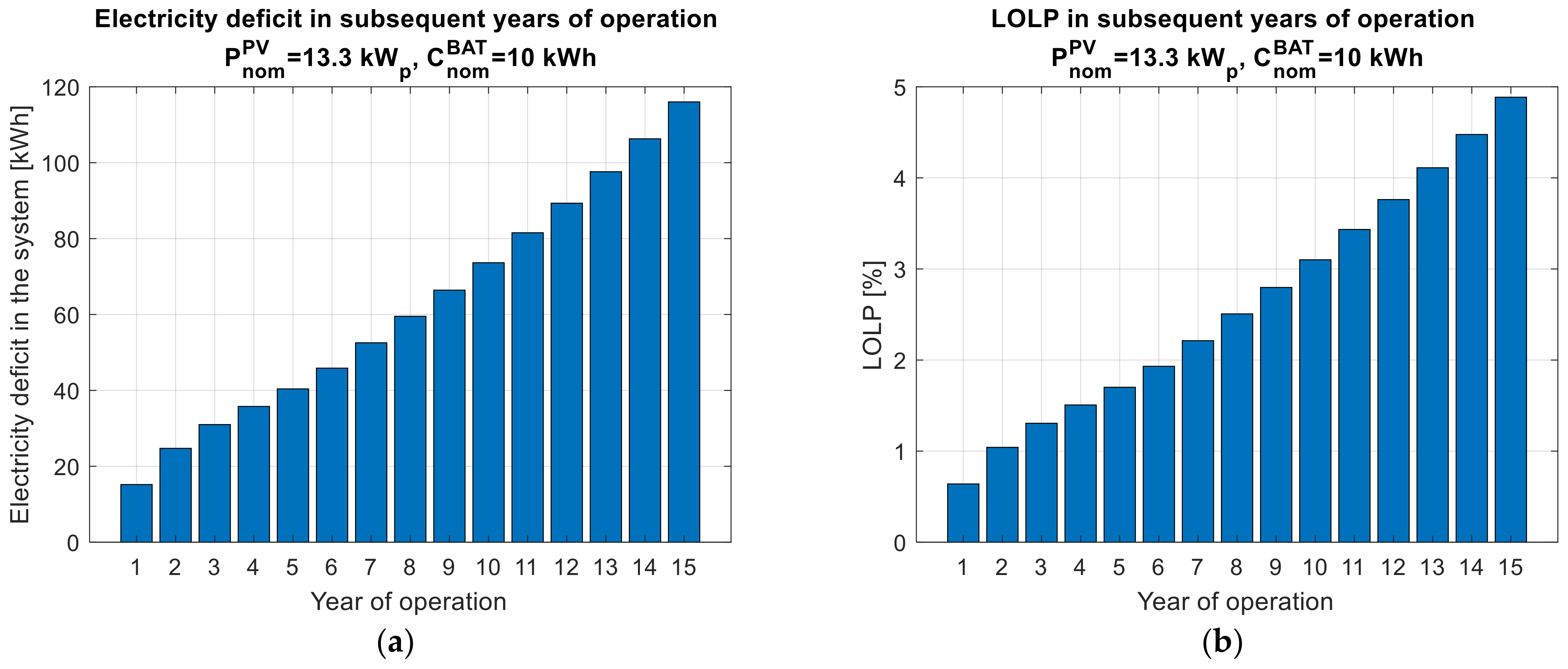
Figure 18 and Figure 19 present the values of key parameters in subsequent years of operation for the best variant of the system configuration, considering degradation (10 kWh, 13.3 kW_p).

Figure 18a shows the deepening of the energy deficit over time, caused by a decrease in the performance of the system components. The energy deficit increased from less than 20 kWh in the first year of operation to almost 120 kWh in the last year of operation. By relating the annual energy deficit to the total annual energy demand (2375 kWh), it can be concluded that the LOLP indicator increased from less than 1% in the first year of operation to almost 5% in the last year of operation (Figure 18b).

The growing energy deficit affects the balance of covering the load demand in the system (Figure 19a). The demand for electricity is less and less covered with the photovoltaic installation and the battery. Figure 19b shows a graphical presentation of the balance of energy generated with the photovoltaic installation. Along with the gradual degradation over the years of operation, the share of unused potential decreases. However, it is still significant and several times higher than the energy used to cover the load demand and charge the battery. However, system oversizing is necessary to ensure the desired level of reliability. System oversizing can be reduced by applying a more liberal reliability criterion, e.g., LOLP ≤ 10%. However, this is associated with greater inconvenience for the user.

Figure 20 shows the progressive degradation of the battery over the years of operation, expressed as a decrease in the available battery capacity.

In this case, the battery operates in a wide range of rated capacity (25–100%), which has a negative effect on the rate of degradation: after 15 years of operation, the available capacity decreases to about 78% of the initial capacity. Such a battery should be replaced.

3.7. Technical and Economic Relationships

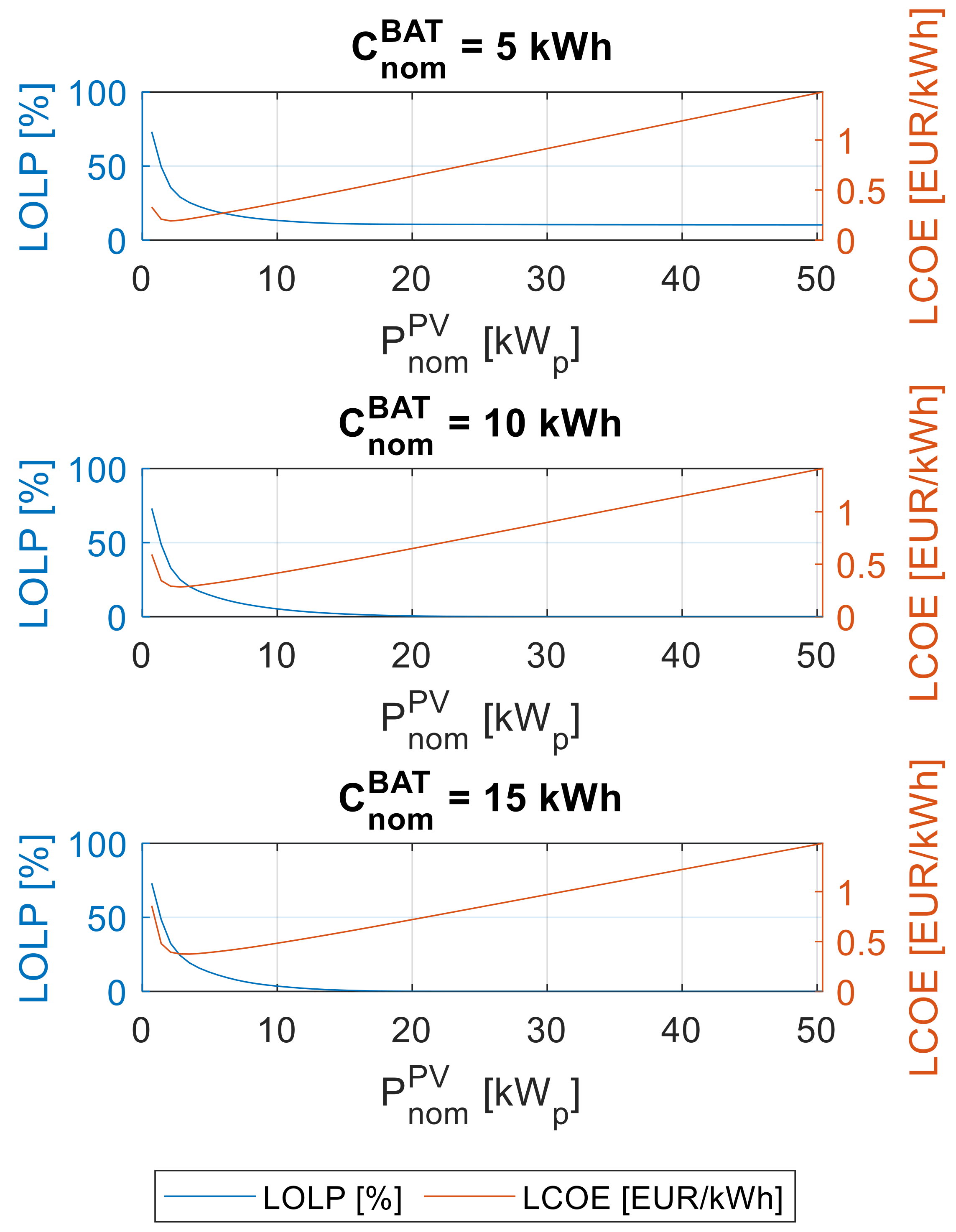
Figure 21 shows the dependence of the LOLP and LCOE indicators on the installed power of the photovoltaic installation for selected variants of the rated storage capacity.

For the selected nominal battery capacity, the LOLP decreases with increasing installed power of the photovoltaic installation. This means that the reliability of the system increases. With a sufficiently large battery capacity, the LOLP decreases even to zero, but when the capacity is too small (e.g., 5 kWh), the LOLP reaches a certain limit. This means that from a certain level, further increases in the installed power of the photovoltaic installation have no effect on the reliability of the system.

For each nominal battery capacity, there is a value of the installed power of the photovoltaic installation at which the LCOE reaches its minimum. For lower values of installed power, the LCOE increases due to the low generation capacity of the system in relation to the demand. On the other hand, for higher installed power values, the LCOE indicator increases because the installation is oversized, and it is necessary to limit the power generation using the PV installation.

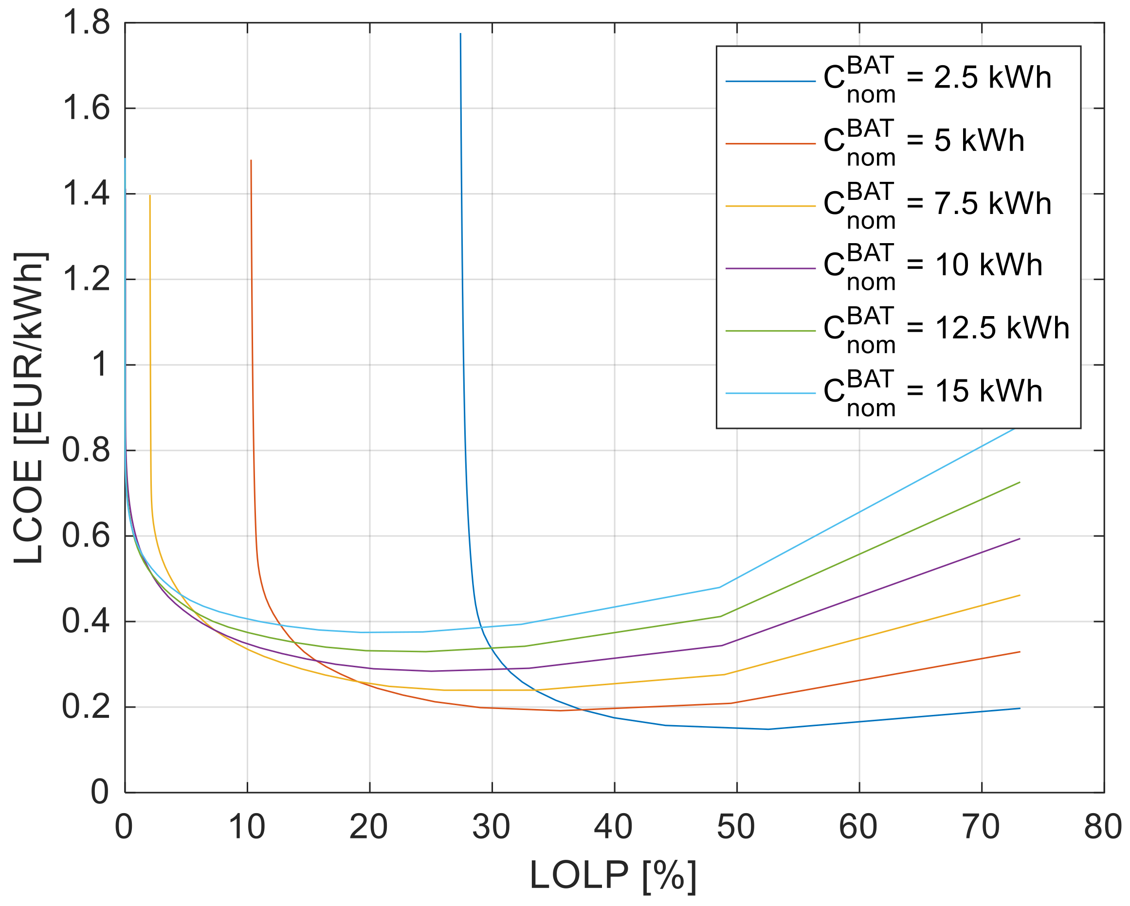
Figure 22 presents the interdependence of the LOLP and LCOE indicators for several selected variants of the nominal storage capacity.

As seen in the data presented in Figure 16, there is a limit value of the LOLP indicator for each nominal battery capacity, at which the LCOE value increases sharply due to the oversizing of the power generation system. On the other hand, the LCOE also increases slightly as the LOLP value increases. This situation occurs when the power and capacity of the system components are underestimated. As shown in Figure 22, the minimum LCOE occurs for LOLP of about 20–50%, which is unacceptable in many cases and applications. Therefore, it should always be considered to oversize the system according to the user’s needs.

4. Discussion

The analysis of the operation of the power generation system consisted of performing simulations for all configurations in the search space and for each year of operation, followed by an update of the parameters related to the performance of the devices. The benefit of the presentation of the results, made possible by using the numerical method, is the graphical visualization of the selected variants of the configuration of the considered power generation system and the selected years of operation. The presentation method allows the observation of changes in key functions and parameters due to degradation, i.e., the waveform of the power and energy deficit; the current state of the energy stored in the battery; the balance of power and energy covering load demand in the system; the balance of power and energy generated with the photovoltaic installation; etc. The results of the simulation tests allow us to carry out the sizing process. It leads to the selection of a configuration that meets the reliability criterion in the last year of operation and achieves the lowest value of the economic indicator.

Based on the simulation results presented in this article, it can be observed how the modelled degradation processes affect the operation of the power generation system over the years of operation. As the number of battery cycles increases, the available capacity of the battery, that is, its ability to store electricity generated with the photovoltaic system, decreases. At the same time, the decrease in energy yield from the photovoltaic installation due to the degradation of the modules increases the demand for electricity from the battery, leading to its more frequent and deeper discharge. As a result of the decrease in the performance of photovoltaic modules and the decrease in charging and discharging efficiency of the battery and the decrease in the available battery capacity, the ability of the system to generate a certain amount of electricity sufficient to cover the load demand decreases with each passing year. Increasingly, over the years of operation, this manifests itself in the presence of a power deficit in the system, which translates into a growing electrical deficit and a growing LOLP reliability indicator on an annual basis.

Naturally, the occurrence of power and electricity deficits over the years of operation can be reduced by appropriately oversizing the system, increasing the installed power of the photovoltaic installation, and/or the nominal capacity of the battery. However, oversizing has the consequence of increasing the unused potential in the balance of energy generated with the photovoltaic installation, stemming from the lack of correlation between the solar irradiation profile and the consumer’s power demand. Improving reliability also requires higher costs, which manifests itself in an increase in the economic LCOE indicator. The aim of the presented methodology is to indicate a compromise between the technical oversizing of the power generation system in order to ensure the required level of reliability in the future and the costs necessary to achieve this goal.

Using a comparative analysis, the results of the sizing process were compiled: the installed power of the photovoltaic installation, the nominal capacity of the battery, and the economic indicator. The results of the sizing process with and without degradation were compared. Using the presented comparative analysis, the necessary scale of oversizing the system was estimated in technical and economic terms. Therefore, the reason for oversizing the system was proven, which is to take degradation into account in the sizing process in order to ensure the desired level of reliability in the long term. In other words, the comparative analysis proves that the degradation of components in the long term affects the obtained test results.

Both the graphical presentations of the operation of the PV/BAT system and the final comparative analysis clearly show the importance of taking degradation processes into account in research on the sizing and planning of the operation of power generation systems based on renewable energy sources operating in an off-grid mode. Neglecting the decrease in component performance in long-term analyses of the operation of the PV/BAT system leads to results reflecting only the initial conditions of the system’s operation. Such an approach, in the case of an off-grid system, leads to the inability to cover the customer’s demand for power and electricity in the subsequent years of operation. Considering aging processes as early as the design stage, and properly oversizing of the system, helps to prevent this.

The aforementioned possibility of observing the impact of degradation on key parameters, waveforms, and technical and economic indicators of the planned power generation system is attractive primarily to potential investors because it supports informed correction of investment decisions. The proposed methodology may therefore prove useful to investors considering a certain degree of oversizing if it is important for them to ensure the desired level of reliability over the years of operation.

It should be noted that the presented methodology, such as any other method present in the literature, has some limitations. These primarily include the adopted load profile specific to a given customer; the adopted meteorological profile depending on the location; the adopted range of the search space dependent on the size of the installation; and installation step which defines the accuracy of the results obtained. In addition, the results of the simulation tests carried out depend on a number of adopted values of technical and economic parameters, i.e., efficiency, power temperature coefficient or unit investment, and operating expenditures. However, while developing the model in a Matlab environment, the authors tried to ensure that its versatility was maintained as much as possible. All the presented simulations and analyses can be carried out by entering arbitrary values of input data waveforms, parameter values, and also by simply adjusting the range and step of the search space. The user is limited only by the hardware requirements related to the use of computer memory and calculation time.

5. Conclusions

This article considers an alternative approach to the process of sizing an independent system consisting of a photovoltaic installation and an electrochemical energy storage. As the traditional method does not consider degradation, the proposed modification of the sizing process of this system consists of conducting long-term analyses, considering the degradation of components. This allows the system to be appropriately oversized to ensure the desired level of reliability after years of operation.

For the PV/BAT system simulation and sizing example presented in this article, it was estimated that ensuring reliability at the level of LOLP = 5% after 15 years of operation requires oversizing the installed power of the photovoltaic installation by 18.75% (from 11.2 kW_p to 13.3 kW_p) and the nominal battery capacity by 33.33% (from 7.5 kWh to 10 kWh). The technical oversizing in the considered case translates into an increase in the cost of electricity of the system, as expressed by the LCOE indicator, by 19.5% (from EUR 0.41/kWh to EUR 0.4899/kWh). The results obtained show the importance of considering degradation in the dimensioning process.

The authors plan to continue research on the impact of the battery capacity used on the results of simulated system operations. Future studies will include an analysis of the system’s operation in the long-term perspective, considering degradation at a rate that depends on the adopted mode of operation (the range of use of the available battery capacity).