Interdecadal Variation Trend of Arctic Wind Energy

Abstract

The Arctic’s navigation and utilization have garnered global interest due to the economic and strategic significance of its open shipping routes. The feasibility and cost-effectiveness of Arctic wind power generation depend largely on the potential of wind energy, which in turn influences the construction of new ports. In order to effectively harness polar wind energy, we must understand and adapt to its ever-changing rules. This study leverages ERA5′s 40-year wind field data to estimate the Theil–Sen Median slope and perform Mann–Kendall trend analysis. We consider factors such as wind power density, effective wind speed occurrence, energy level frequency, stability, and resource reserves to comprehensively analyze the intergenerational variations in Arctic wind energy resources. Our findings indicate that Northeast Passage, Davis Strait, and Baffin Bay possess favorable wind power density (1~2 W/m²·yr⁻¹), effective wind speed occurrence (0.1~0.2%·yr⁻¹), energy level frequency (0.1~0.2%·yr⁻¹), stability (−0.005 yr⁻¹), and resource reserves (1 kWh/m²·yr⁻¹). However, these indicators are inferior in the Barents Sea, Canada’s northern archipelagos, and Greenland’s vicinity, where wind energy is relatively poor and unfavorable for development. Autumn dominates the annual change trend of Arctic wind energy, while spring and summer show no significant trends.

1. Introduction

In recent years, the Arctic has become a valuable region due to its abundant resources and highly profitable shipping routes; the melting of sea ice caused by global warming intensifies these benefits. The opening of Arctic shipping routes can change the current world shipping pattern and bring tremendous economic benefits [1,2,3,4,5,6]. However, the construction of fewer ports in the Arctic relies heavily on traditional fossil energy for supplies, which pollutes the entire Arctic and harms the global climate through emissions of pollutants. Additionally, the Arctic plays a crucial role in global thermal balance and acts as a “magnifier” for amplifying signals of climate abnormalities [7,8,9]. Therefore, it is essential to develop sustainable technologies that rely on renewable energy sources to protect the Arctic’s unique environment and ensure long-term economic development. Offshore wind power generation can not only reduce air pollution in coastal areas [10] but also ensure the sustainable development of scientific research activities. The benefits of wind energy mining in the Arctic include the construction of new ports, resource relief along routes, and improved navigation. Researchers have developed models to evaluate the economic feasibility of offshore wind farms in Finland [11] and a hybrid renewable energy system that can meet single households’ energy demands in the Arctic [12]. Wind energy plays a crucial role in creating conditions for social and economic development in the Murmansk region [13], while national policies prioritize renewable energy but face both opportunities and challenges [14]. Alaska’s wind energy systems are an essential resource for rural and remote communities that currently rely on diesel power generation and heating [15].

Esmaeili et al. [16] used 10-year data from Iran’s northern weather stations and proposed new parameters, including Exponentiated Half-Logistic (EHL), Exponentiated Half-Normal (EHN), Skew Logistic (SKL), and Generalized Extreme Value (GEV), to improve the accuracy of wind speed forecasts. The GEV was found to be well-matched with the data. The highest wind power density sites are located in Ardabil, Gorgan, and Zanjan. Zheng et al. [17] identified six common bottlenecks in current energy classification schemes, including inconsistencies with physical mechanisms, inability to meet diverse task requirements, and applicability issues in certain seasons/months. To address these challenges, a dynamic adaptive wave energy classification scheme that takes into account various factors is adaptable for different tasks, is available at any time, and is suitable for use across regions has been proposed. Wind energy development can draw on the categorization scheme used in wave energy development to present bottleneck challenges and propose solutions. Kay [18] defined Wind drought events and calculated their probability using large-scale climate models and observation records. He found that the probability of three or more consecutive weeks of wind drought in winter is 1/40.

Costoya et al. [19] found that China’s coastal areas will have abundant wind energy resources in the coming decades, based on offshore buoy wind field data and ERA5 data. Duan et al. [20] used ERA intermediate wind field data from 1996 to 2015 to analyze the wind energy resources in ice-free areas of the Barents Sea and described the distribution of wind energy resources and extreme wind speed in the Barents Sea. AKPEROV et al. [21] used ERA5 wind field data and RCA4 regional climate model to obtain the distribution of wind power density in the Arctic and pointed out that WPD increased significantly in winter, especially in the Barents Sea, Kara Sea, and Chukchi Sea. Human activities have a more significant impact on wind energy changes. Ghani et al. [22] used NOAA data and Computational fluid dynamics numerical simulation method to assess the wind energy resources of the Solowitsky Islands. It was pointed out that the Solowitsky Islands have higher wind power generation in winter.

Decastro et al. [23] noted differences in the development of offshore wind energy between Europe, China, and the United States, with Europe currently leading the way. China is rapidly developing offshore wind energy, while the US depends on regulatory measures. Wills et al. [24] used the meteorological station data in northern Canada to combine the simulation of solar and wind power generation systems with similar capacity with historical data to compare and contrast power generation potential and support renewable energy deployment. Xydis [25] analyzed wind fields in northern Greece to optimize the layout of wind farms for agricultural purposes. Minin and Tselishcheva [26] found an increase in wind speeds along the Arctic coast, with the strongest winter winds. They also explored the joint work of wind power generation, diesel power plants, and boiler plants.

Some scholars have investigated the distribution and development of wind energy resources in the Arctic [21,22,24,26], but there are several challenges. Firstly, the research is not comprehensive enough as most analyses focus on specific areas or archipelagos, lacking a holistic view of the region’s wind energy resources. Secondly, data coverage is limited. While satellite observation methods have improved, historical data for the Arctic remain scarce. Thirdly, analysis methods are not always scientific. Some researchers use linear trends when examining trends, which can be misleading [27,28]. In this study, we utilized the ERA5 reanalysis data from ECMWF to evaluate the wind energy resources in the Arctic region. We employed Theil Sen Median slope estimation and Mann–Kendall trend analysis to calculate the interdecadal variation trend of key indicators of wind energy. Our aim is to grasp the potential of Arctic wind energy development and actively respond to national goals of “carbon peak” and “carbon neutrality”. By doing so, we hope to draw attention to the development and utilization of wind energy resources in the Arctic region, increase the use of clean energy, and promote sustainable development in the area.

2. Materials and Methods

2.1. Study Area

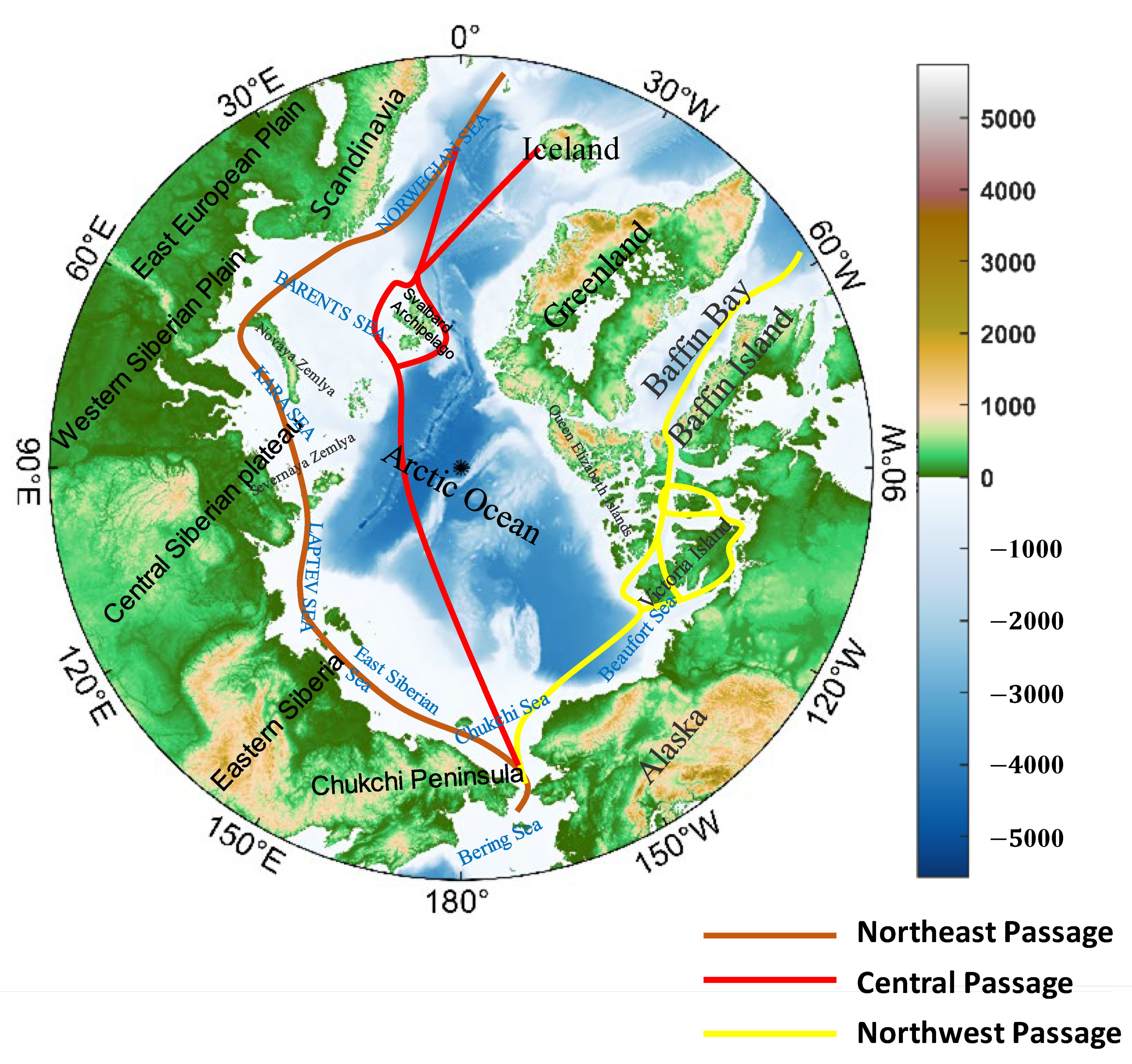
As shown in Figure 1. The study covers the Arctic Ocean and its coastal regions. The commonly referred to as the North Pole refers to the area north of 66.5° N. This article selects an area north of 60° N, covering the Arctic Ocean, coastal countries’ land, and the Arctic inland sea. The Arctic is divided into three sections: the Northeast Passage, Northwest Passage, and Central Passage. The land around the Arctic Ocean can be divided into two parts: Eurasia and North America and Greenland. Bering Strait separates these two parts of the land area. Due to global warming, the Arctic Passage is becoming navigable. The Arctic Passage is a vital sea route connecting the Pacific and Atlantic oceans, and it is also a newly developed shortest sea transportation channel connecting Southeast Asia and Europe. The opening and utilization of the Arctic navigation channel have become a significant issue that has garnered international attention.

2.2. Methods

The formula for calculating wind power density is as follows:

$$W=\frac{1}{2}\rho V^3$$

(1)

In Formula (1), $\mathrm{W}$ is wind power density (W/m²); $V$ is wind speed (m/s); $\rho$ is sea surface air density. If the altitude is less than 500 m, $\rho$ is 1.225 kg/m³.

In the process of ocean engineering construction, the frequency of strong wind has a great impact on work efficiency and even damages the safety of personnel and equipment in severe cases. It also determines the take-off and landing of aircraft and other platforms [29,30]. In the process of wind energy resource development, the frequency of strong wind can also indicate the level of wind energy resources. This paper adopted the definition of effective wind speed occurrence (EWSO) proposed by Zheng [31,32] with a consideration that wind speed between 5 and 25 m/s is favorable to collection and conversion of wind energy.

$$EWSO=\frac{t_1}{T}\times 100\%$$

(2)

In Equation (2), EWSO is the effective wind speed occurrence, t₁ is the occurrence time of effective wind speed, and T is the total time.

Selecting the frequency of ALO (Available Level Occurrence, >100 W/m²), RLO (Rich Level Occurrence, >200 W/m²), and SLO (Superb Level Occurrence, >400 W/m²) as evaluation indicators for Energy Level Occurrence, Energy Level Occurrence can display the richness of wind energy at all levels, and calculating its evolution trend can represent the evolution trend of wind power density at all levels.

$$ALO=\frac{t_{100}}{T}\times 100\%$$

(3)

$$RLO=\frac{t_{200}}{T}\times 100\%$$

(4)

$$SLO=\frac{t_{400}}{T}\times 100\%$$

(5)

In Equations (3)–(5), t₁₀₀, t₂₀₀, t₄₀₀ are the times when the wind power density is above 100, 200, and 400 W/m², respectively, and T is the total time.

Zheng et al. [31,32] used the coefficient of variation (C_v), Monthly Variability Index (M_v), and Seasonal Variability Index (S_v) to demonstrate the stability of wind energy resources. The stability and dispersion degree of wind power density are also significant indicators for evaluating and utilizing wind energy [33,34]. Stable wind power density is beneficial for the development and utilization of wind energy, resulting in increased exploitation benefits. In contrast, unstable wind energy can cause damage to instruments and equipment and even lead to safety accidents. The larger the C_v value is, the greater the variation amplitude of wind energy, indicating poor representativeness and instability. Otherwise, wind energy is stable. When C_v value is greater than 1, the average range of wind energy variation is greater than the average, indicating poor representativeness.

$$C_V=\frac{S}{\overline{X}}$$

(6)

$$S=\sqrt{\frac{{\displaystyle \sum _{i=1}^n{X}_i^2}-{\left({\displaystyle \sum _{i=1}^n{X}_i}\right)}^2/n}{n-1}}$$

(7)

In Equations (6) and (7), $C_v$ is the coefficient of variation, $\overline{X}$ is the mean value, S is the standard deviation, and n is the number of samples.

$$M_v=\frac{P_{M1}-P_{M12}}{P_{year}}$$

(8)

In Formula (8), $P_{M1}$ is the wind power density of the most abundant month, $P_{M12}$ is the wind power density of the poorest month, and $P_{year}$ is the average wind power density of the years.

$$S_v=\frac{P_{S1}-P_{S4}}{P_{year}}$$

(9)

In Formula (9), $P_{S1}$ is the wind power density of the most abundant season, $P_{\mathrm{S}4}$ is the wind power density of the least abundant season, and $P_{year}$ is the average wind power density of the years.

Using Zheng et al. [31,32] calculation method for wind energy resource reserves, calculate the total wind energy resource reserves in the Arctic region, and use the wind speed effective wind speed occurrence and total wind energy reserves to calculate the effective wind energy resource reserves.

$$E_{PT}=\overline{P}\times H$$

(10)

$$E_{PE}=\overline{P}\times H_E$$

(11)

In Formula (10), $E_{PT}$ is the total wind energy reserves, $\overline{P}$ is the average wind power density, $H$ is the annual hours; In Formula (11), $E_{P\mathrm{E}}$ is the effective storage of wind energy, $\overline{P}$ is the average wind power density, $H_{\mathrm{E}}$ is the number of hours during which the effective wind speed occurs throughout the year.

The wind power density in March 1981 was averaged to the average wind power density in March 1981 in the Arctic region, and the average wind power density in 12 months in the past 40 years was obtained according to the same method. Other indicators obtained data for nearly 40 years using the same method.

Calculate indicators such as wind power density, effect wind speed occurrence, energy level frequency, stability, and resource reserves proposed by Zheng et al. We used Theil–Sen Median slope estimation to analyze the Mann–Kendall trend in these indicators by using annual and seasonal average index data over a 40-year period. Theil–Sen Median slope estimation is a highly efficient method that is less sensitive to measurement errors and outliers and is often used for long-term series data trend analysis [35,36]. Mann–Kendall test is a nonparametric test method that does not require a specific distribution and is less affected by outliers, making it suitable for ordinal variables. It has been successfully applied in hydrological and meteorological trend changes to determine the significance of temperature, runoff, precipitation, climate, and other changes [37,38,39,40].

2.3. ERA5 Reanalysis Data

The dataset used in this study is the ERA5 reanalysis data provided by ECMWF. ERA5 Contains detailed data on global atmosphere, land, and ocean waves since 1950, replacing ERA-interim. ERA5 is a new-generation reanalysis dataset with hourly resolution. Compared to ERA-interim, ERA5 has twice the accuracy of spatial resolution, and various forecasting and assimilation integrated models are more scientific and advanced [41].

It covers a wide range of products from 1940 to the present, with a spatial resolution of 1/4° and hourly accuracy, providing global coverage. ERA5 is a new-generation product widely used in meteorological and oceanographic data analysis [42,43]. It has a smaller bias than other datasets and has been verified for its accuracy at high latitudes by many scholars [44,45,46]. Compared to other datasets, ERA5 has been proven by many scholars to have good accuracy and high degree of fitting. ERA5 datasets can also fit variables such as temperature, wind field, ozone content, etc., in high-latitude regions well [47,48,49,50]. The dataset selected in this study covers the region between 60° N and 90° N with a spatial resolution of 1/4° and a temporal resolution of every 6 h. The focus of this study is to use reanalysis datasets to reveal the historical trend of wind energy density in the Arctic without taking into account sudden changes in wind speed caused by sudden weather phenomena such as cold eddies and cyclones. The data need to be processed evenly. Selecting the data at 0000, 0600, 1200, and 1800 can basically represent the wind speed data within a day.

3. Variation Trend of Arctic Wind Energy

3.1. Wind Power Density

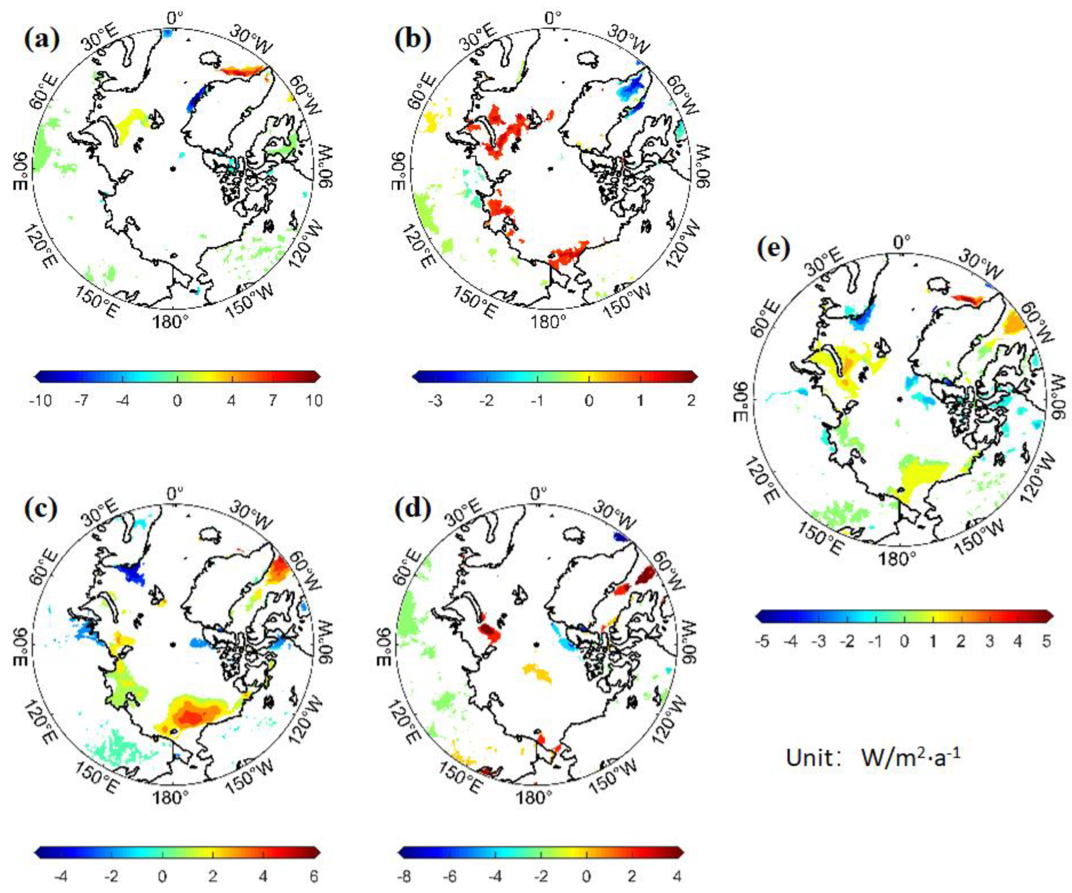
The wind power density in the spring of 40 years was calculated by the Theil–Sen Median trend and Mann–Kendall trend analysis, and the variation trend of the wind power density in four seasons and the average annual year in the Arctic were obtained, as shown in Figure 2.

WPD Annual Variation: The Arctic displays a consistent pattern of increasing wind power density, with the most notable increases occurring in close proximity to the Chukchi Sea, Novaya Zemlya (1~2 W/m²·yr⁻¹), Denmark Strait (3~5 W/m²·yr⁻¹), and Davis Strait (2 W/m²·yr⁻¹). However, there are also regions where wind power density is significantly decreasing, mainly in the Barents Sea (−2~−5 W/m²·yr⁻¹), northern Greenland (−1~−2 W/m²·yr⁻¹), and near the Parry Islands (−2 W/m²·yr⁻¹).

Seasonal Trends: In spring, there is no clear change in the Arctic wind power density. The regions with significant increases are distributed in the Barents Sea (2 W/m²·yr⁻¹), Davis Strait (4~7 W/m²·yr⁻¹), and the regions with significant decreases are distributed in the North Sea (−4 W/m²·yr⁻¹), Greenland Sea (−10 W/m²·yr⁻¹), and Queen Elizabeth Islands (−2 W/m²·yr⁻¹). During summer, the northeast waterway shows an increasing trend along the coast. The regions with significant increases are near the Chukchi Sea, Laptev Sea, and Novaya Zemlya Svalbard Islands (1~2 W/m²·yr⁻¹), while the regions with significant decreases are distributed in Central Siberia (−0.5 W/m²·yr⁻¹) and Greenland (−1~−3 W/m²·yr⁻¹). Autumn brings positive changes to the Arctic wind power density, with regions of increase in Chukchi Sea (1~4 W/m²·yr⁻¹), Laptev Sea (1~2 W/m²·yr⁻¹), Davis Strait (3~4 W/m²·yr⁻¹), and negative trends in Northern Canada Islands, Gulf of Ob (−2 W/m²·yr⁻¹), and Barents Sea (−4 W/m²·yr⁻¹). Winter brings positive trends to Chukchi Sea (2 W/m²·yr⁻¹), Kara Sea (2~4 W/m²·yr⁻¹) and Baffin Bay (2~4 W/m²·yr⁻¹), while negative trends are found in the Western European Plain, Siberia, and other places (−2 W/m²·yr⁻¹), Ellesmere Island (−4 W/m²·yr⁻¹), and near the south of Greenland (−6~−8 W/m²·yr⁻¹).

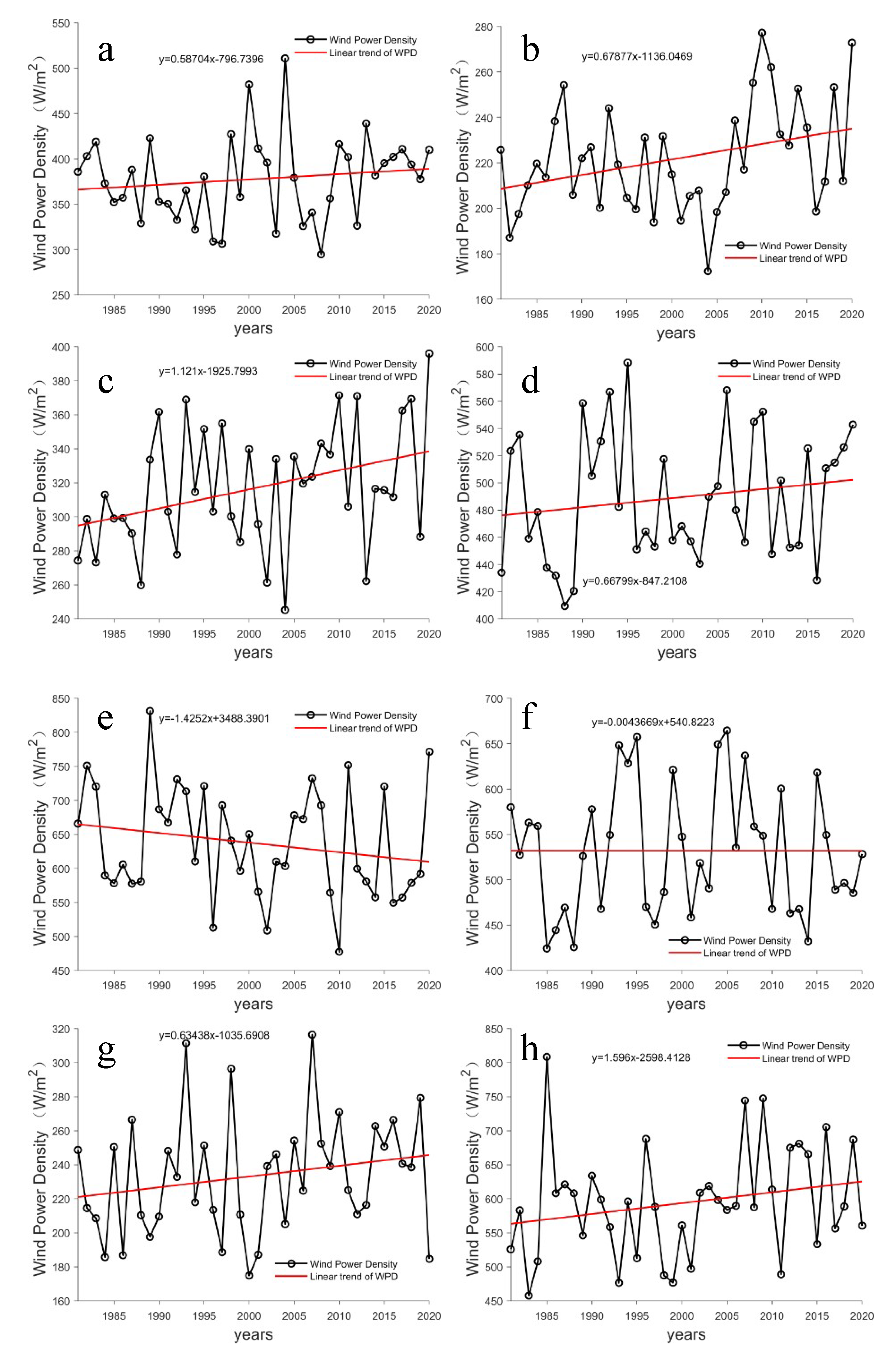
Comparing seasonal and annual trends, we observe that the Chukchi Sea maintains a positive trend throughout the year, with autumn as its primary season. The Barents Sea exhibits a positive trend during summer, while northern Norway experiences a decreasing trend in autumn. Baffin Bay displays an increasing trend in autumn and winter. Figure 3 shows the time series of wind power density in the inland waters of the Arctic region, showing a positive trend in all regions except for the Norwegian Sea.

The positive trends observed in the Chukchi Sea and Beaufort Sea in autumn are related to the abnormal SLP of the North and South Dipoles and the enhanced polar atmospheric circulation caused by the greenhouse effect, which in turn leads to a significant increase in wind energy in the region [51]. Zhang et al. [52] showed that sea ice leads to a negative correlation between wind speed and sea surface temperature in open water; There is a positive correlation in areas with dense sea ice. In open areas close to land, there is a positive correlation between wind speed and sea surface temperature. As the greenhouse effect leads to a gradual increase in polar sea surface temperature, wind speed in areas such as the Chukchi Sea and the Beaufort Sea shows a significant increasing trend.

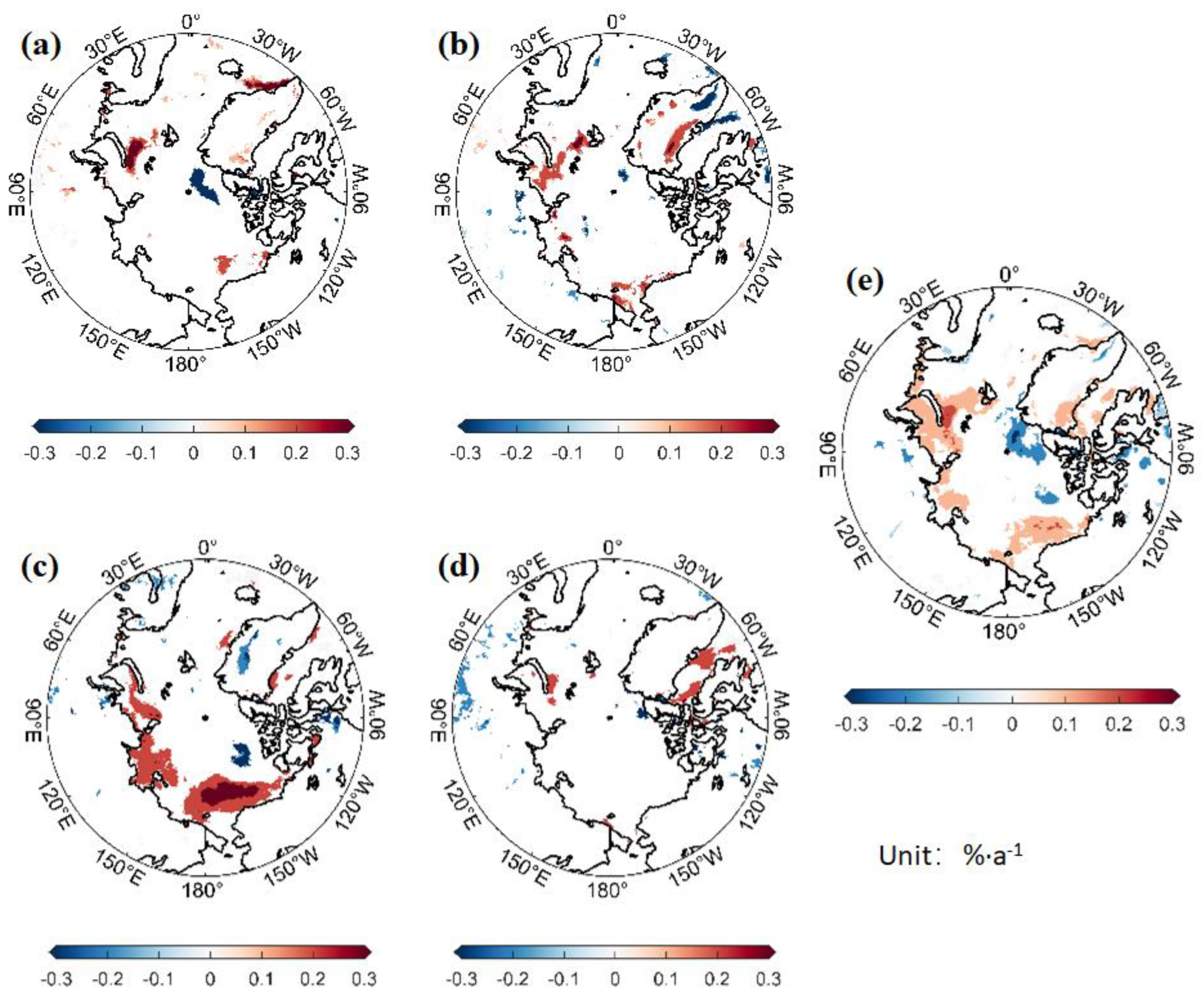
3.2. Effective Wind Speed Occurrence

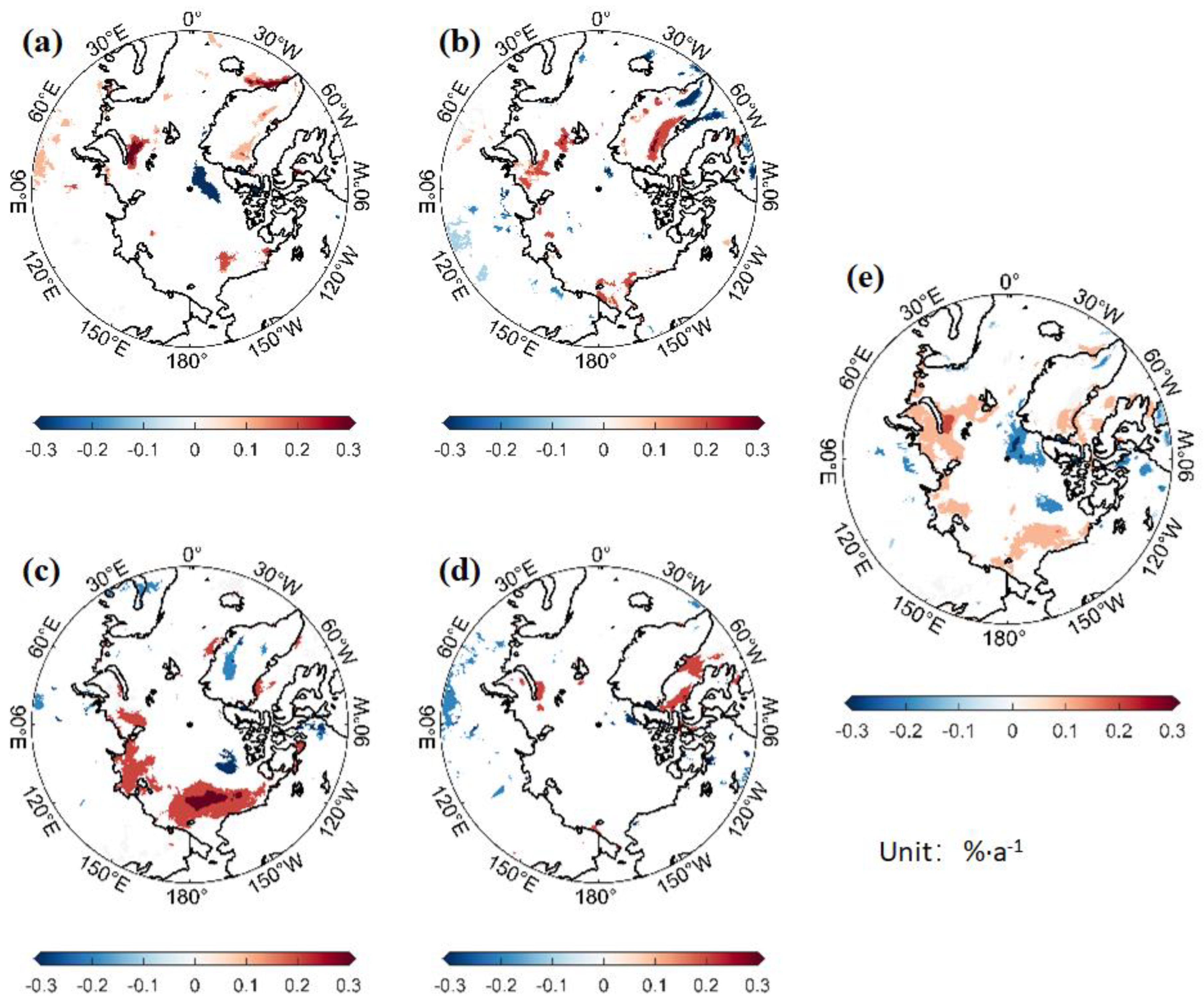
To calculate the evolution of wind power density, we employed a method based on wind speed data from nearly four decades. This approach allowed us to determine the occurrence of effective wind speeds, as illustrated in Figure 4.

EWSO variation trend: The annual change trend of Arctic EWSO presents a positive trend as a whole, with significant increase areas distributed in the Chukchi Sea, Beaufort Sea, Kara Sea, White Sea, Barents Sea, near Greenland, Baffin Bay, and near Northern Canada Islands (0.1%·yr⁻¹), and an increased center of 0.2~0.3%·yr⁻¹ appears near Novaya Zemlya, with significant decrease areas distributed in northern Greenland (−0.2~−0.3%·yr⁻¹) North of Beaufort Sea (−0.2%·yr⁻¹).

Seasonal variation trend of EWSO: In spring, the Arctic is mainly positive, but the negative trend is relatively strong near Greenland North Pole and Ellesmere Island (<−0.3%·yr⁻¹), and the positive trend is mainly distributed near Novaya Zemlya, the Denmark Strait (0.2~0.3%·yr⁻¹), the Beaufort Sea (0.2%·yr⁻¹), Siberia, and Greenland (0.1%·yr⁻¹). In summer, the positive trend is distributed in the Chukchi Sea, Kara Sea, Barents Sea, northern Greenland, and Hudson Strait (0.2~0.3%·yr⁻¹). The significant decline areas are Siberia (−0.1~−0.2%·yr⁻¹), northern Greenland, and Davis Strait (−0.2~−0.3%·yr⁻¹). In autumn, there is a significant positive trend. The positive trend is distributed in the Chukchi Sea (0.2~0.3%·yr⁻¹), Laptev Sea, Kara Sea, Victoria Island, and the coastal waters of Greenland (0.2%·yr⁻¹). The negative region is distributed in the Beaufort Sea (−0.3%·yr⁻¹), the Gulf of Bosnia, and Greenland (−0.2%·yr⁻¹). In winter, there is no obvious change in the Arctic Ocean region. Positive regions (0.2%·yr⁻¹) appear near Novaya Zemlya, Baffin Bay, Canada’s Northern Isles, and decreasing regions (−0.2%·yr⁻¹) appear in Siberia.

Wind energy in the Arctic exhibits a positive trend overall. The Chukchi Sea’s positive region is dominated by autumn, while spring brings an increasing area near Novaya Zemlya. The decreasing trend of northern Canada’s islands is reflected in spring and autumn.

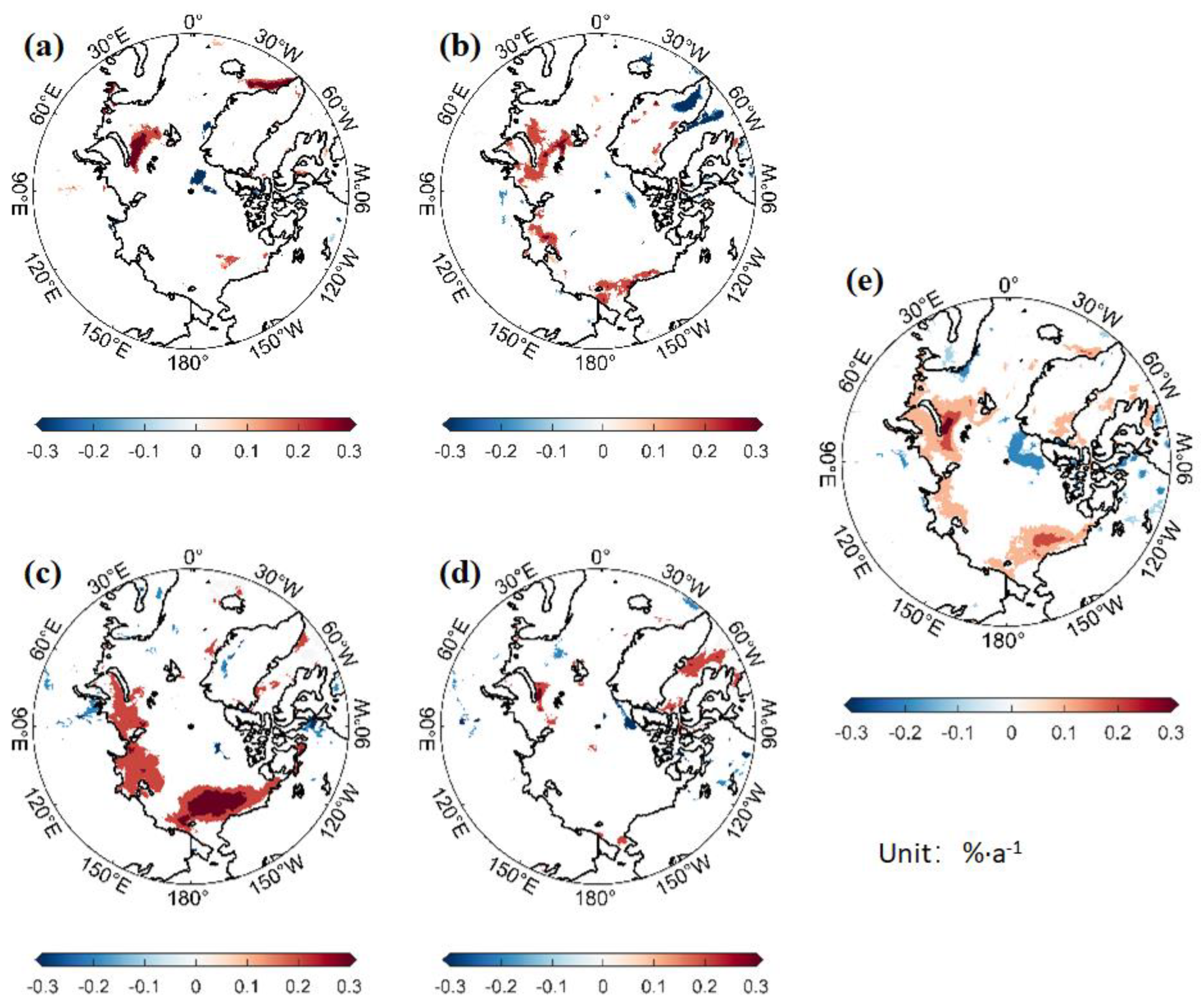
3.3. Energy Level Occurrence

According to the Sen trend and MK test, the interdecadal variation pattern of Energy Level Occurrence is obtained by trending the energy level frequencies obtained in the past 40 years. See Figure 5, Figure 6 and Figure 7 below.

ALO variation: The trend follows a similar pattern to that of EWSO. The positive areas are concentrated in the Chukchi Sea, Laptev Sea, Novaya Zemlya, Baffin Bay, and other locations, while the negative areas are found near Greenland and Northern Canada Islands. ALO refers to wind energy frequency greater than 100 W/m², while EWSO measures between 5 and 25 m/s. The similarity between the two is due to the fact that the high ALO region in the Arctic has a wind speed within the range available.

The distribution of RLO and ALO is basically similar, with a significant difference being that the trend of RLO is more significant. For example, in summer, Greenland shows a more significant negative trend, while the northeast waterway shows a more positive trend. In autumn, the negative trend of RLO basically disappeared, and the positive areas in the Chukchi Sea, Laptev Sea, and Kara Sea further expanded. In winter, the distribution of ALO and RLO is basically consistent. The positive trend around the Chukchi Sea and Novaya Zemlya increases year by year.

SLO and RLO exhibit similar patterns, with the primary distinction being that SLO’s trend weakens and its numerical value decreases. In autumn, the positive region in the Chukchi Sea remains relatively unchanged. The negative areas in Greenland and northern Canada gradually diminish, while a negative area emerges in the Barents Sea. Compared to RLO, Davis Strait’s winter distribution center is further strengthened as it grows increasingly positive.

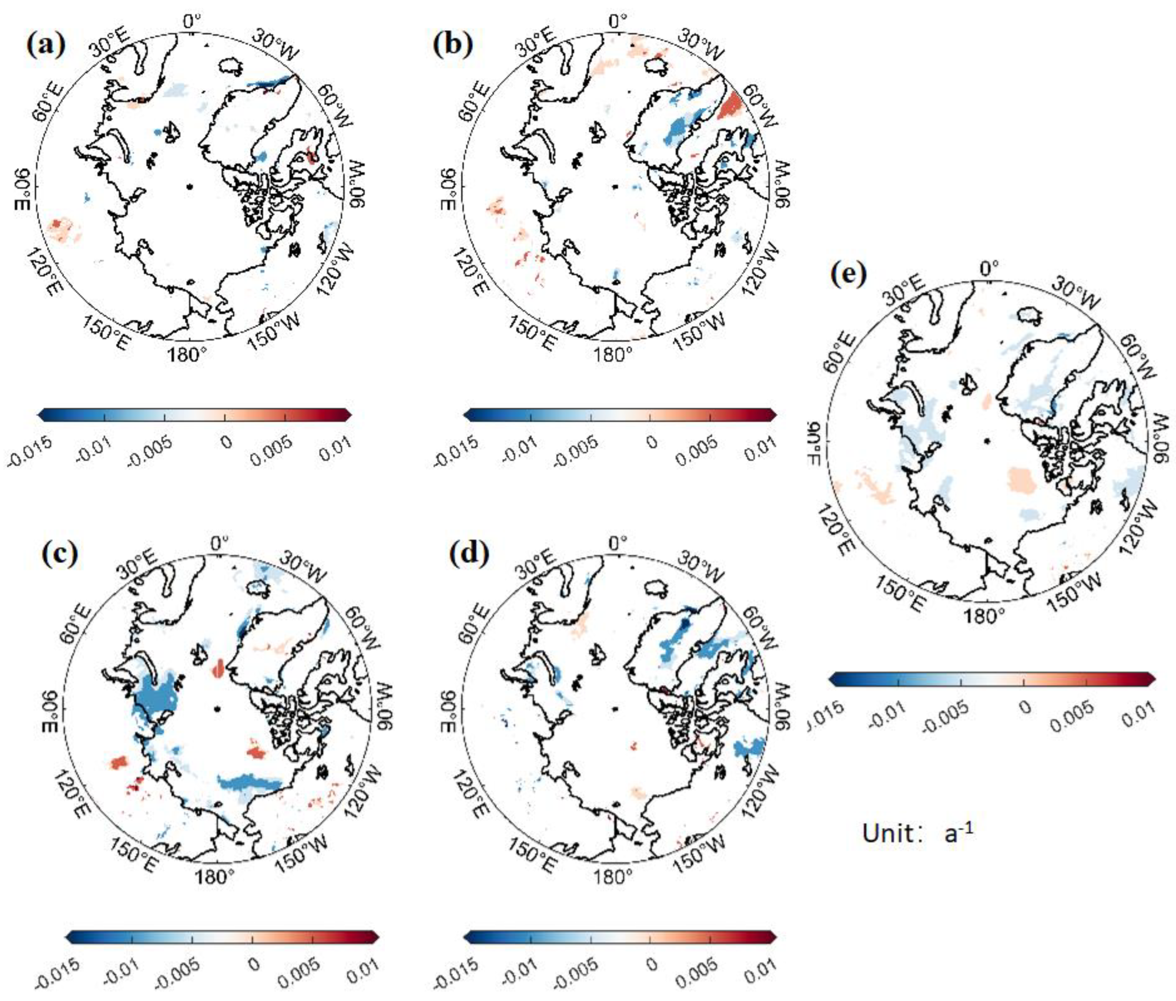
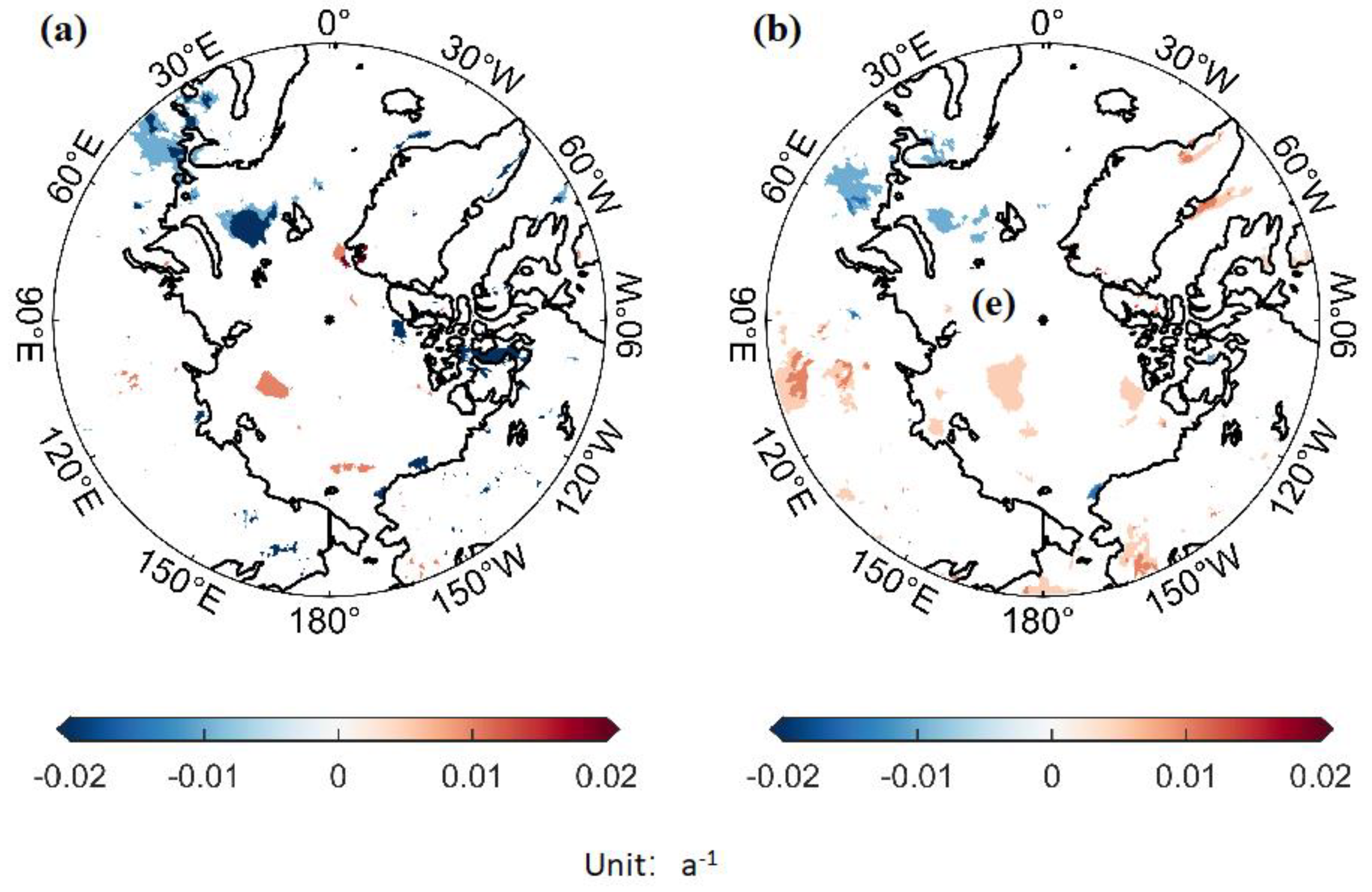
3.4. Stability

As shown in Figure 8. The annual variation of Cv is not evident. The Kara Sea, Greenland, Canada, and other regions exhibit a decline in the coefficient of variation by −0.005 yr⁻¹, indicating that the wind power density tends to be stable in these areas. The occurrence of a positive area of 0.005 yr⁻¹ in the northern part of the Beaufort Sea indicates an increase in the coefficient of variation, which is not conducive to the development of wind energy resources due to its instability. In spring, there is no significant trend in the coefficient of variation in the Arctic, but there is a notable decrease near Greenland (−0.01~−0.015 yr⁻¹). During summer, positive trends are observed in Davis Strait (0.05 yr⁻¹), while negative regions are located in Greenland (−0.01 yr⁻¹). Autumn shows significant decreases in the Chukchi Sea and Kara Sea (−0.01 yr⁻¹), with scattered positive trends. Winter exhibits significant decreases in Greenland, Baffin Bay, and Canada (−0.01 yr⁻¹), which contributes to the stability of wind energy. Overall, the evolution of Cv during autumn and winter seasons mainly exhibits negative trends, contributing to wind energy stability.

M_v variation trend (Figure 9a): M_v represents the monthly difference in wind energy in the region within the year, showing a negative trend indicating that the monthly difference in wind energy gradually decreases, and wind energy tends to stabilize throughout the year, which is conducive to the development of wind energy resources. Figure 9a below shows the evolution trend of M_v. It can be seen that the Arctic has a negative trend as a whole, with significant decline areas in the Barents Sea (−0.02 yr⁻¹), Western European Plain (−0.01 yr⁻¹), and the Northern Canada Islands (−0.02 yr⁻¹). The significantly increasing regions are distributed in the north of the Laptev Sea (0.01 yr⁻¹).

The seasonal variation trend of S_v represents the differences in wind energy between seasons within a year. The negative trend table indicates that these differences will decrease next year, which is beneficial for wind energy development. Figure 9b below shows that S_v has a certain growth trend, with positive trends distributed in Siberia (0.01 yr⁻¹), the Bering Sea, the northern Laptev Sea, the northern islands of Northern Canada (0.005 yr⁻¹), and near Greenland (0.005~0.01 yr⁻¹). However, this increasing trend in these areas is not conducive to the stability of wind energy during the season and hinders wind energy development. Conversely, the negative trend is distributed in the Barents Sea and the Western European Plain (−0.01 yr⁻¹).

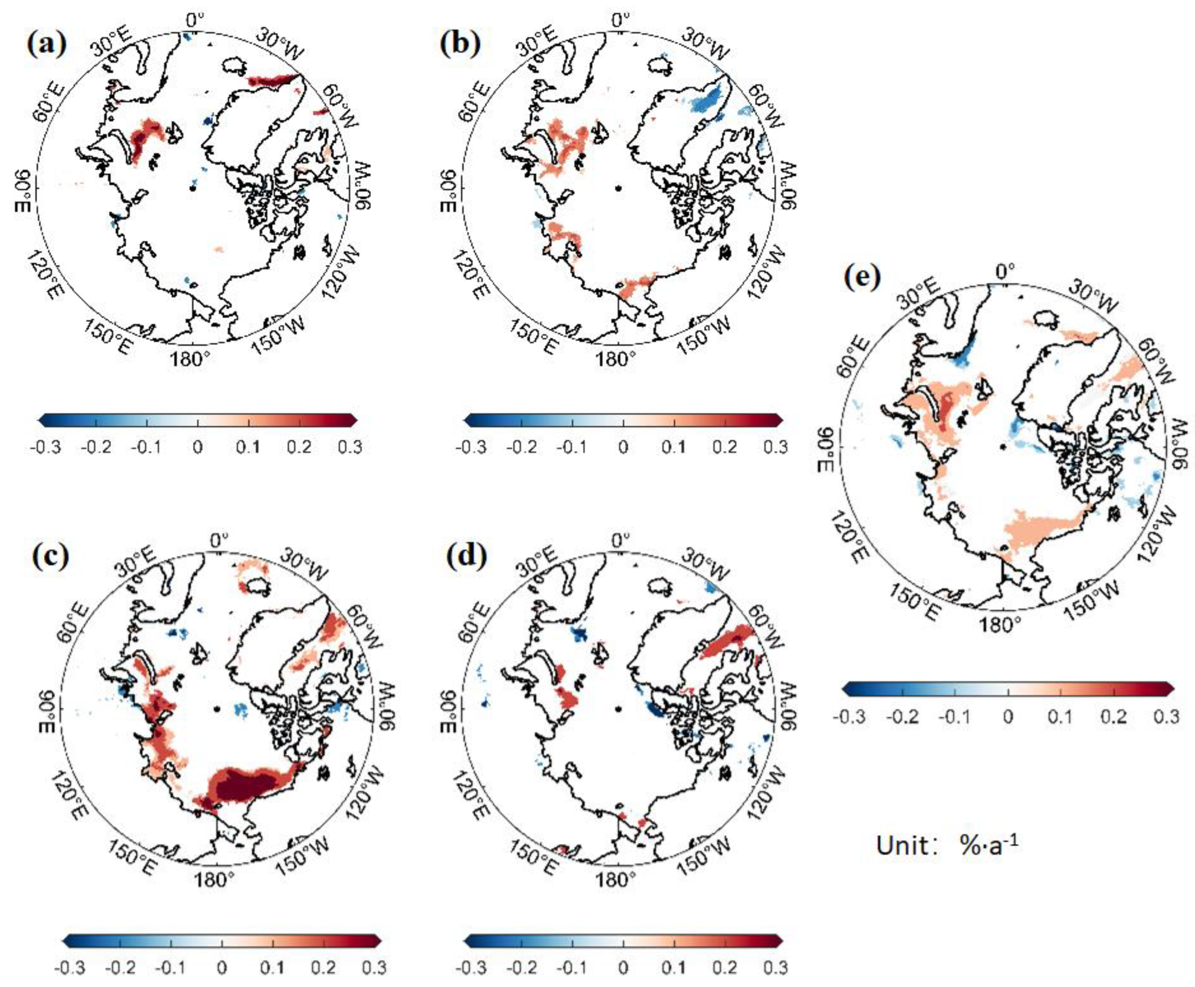
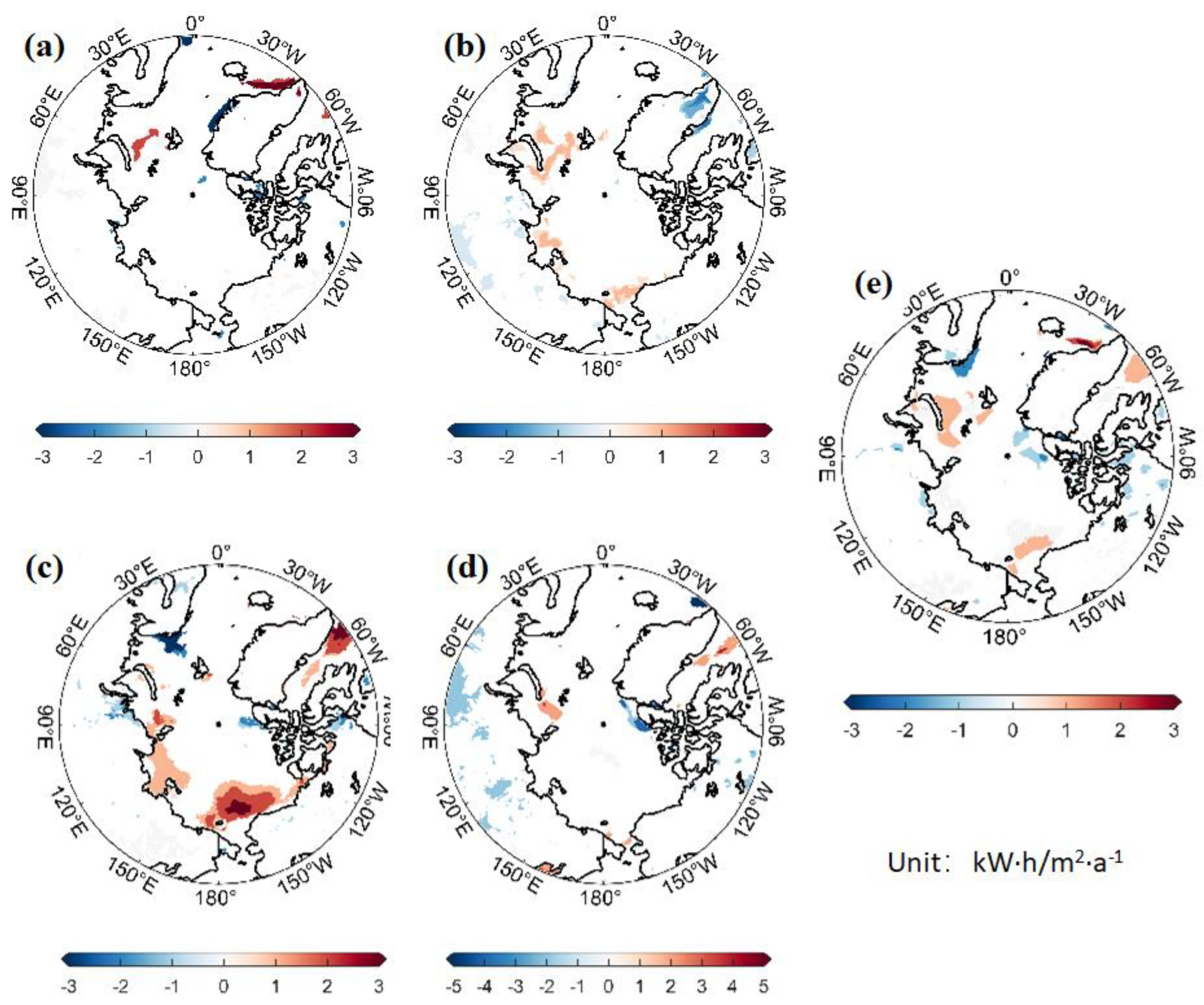
3.5. Energy Resource

Based on the 40a wind energy resource reserves obtained, the evolution trend of the total wind energy resource reserves is calculated through Sen trend calculation and mk test, as shown in Figure 10 and Figure 11.

Total reserves of wind energy resources: The positive growth areas in wind energy resources are located near Chukchi Sea, Novaya Zemlya, Davis Strait (1 kW·h/m²·yr⁻¹), and Greenland (3 kW·h/m²·yr⁻¹). Conversely, the negative growth areas are distributed in the Northern Islands of Northern Canada (−1 kW·h/m²·yr⁻¹) and Barents Sea (−2 kW·h/m²·yr⁻¹). In spring, there is no clear trend area, but the positive area is found in the Barents Sea (2 kW·h/m²·yr⁻¹) and near Greenland (3 kW·h/m²·yr⁻¹). The negative area is spread across the Greenland Sea and the northern islands of Northern Canada (−1~−3 kW·h/m²·yr⁻¹). During summer, the Northeast Passage area (1 kW·h/m²·yr⁻¹) shows a positive trend, while Greenland (−2 kW·h/m²·yr⁻¹), Canada (−1 kW·h/m²·yr⁻¹), and Siberia (−0.5 kW·h/m²·yr⁻¹) show a negative trend. In autumn, active areas are found in the Chukchi Sea (1−3 kW·h/m²·yr⁻¹), Baffin Bay and Laptev Sea (1 kW·h/m²·yr⁻¹), and Davis Strait (2~3 kW·h/m²·yr⁻¹). The negative trend is scattered in the Gulf of Ob (−1 kW·h/m²·yr⁻¹), Barents Sea (−3 kW·h/m²·yr⁻¹), and Northern Canada Islands (−1 kW·h/m²·yr⁻¹). In winter, the East European Plain and Siberia (−1~−2 kW·h/m²·yr⁻¹), the Northern Islands of Northern Canada (−2~−4 kW·h/m²·yr⁻¹) show significant negative trends, while positive growth is observed in the Kara Sea, Davis Strait (2~3 kW·h/m²·yr⁻¹), and other places. The increase in wind energy reserves significantly contributes to wind energy development.

By comparing the seasonal growth trend of the Arctic, we can observe that autumn is the dominant factor driving its transformation. The seasonal change trend for different types of locations, such as the Chukchi Sea, near Novaya Zemlya, Greenland, Barents Sea, and Northern Canada Islands, is similar, but the values have decreased.

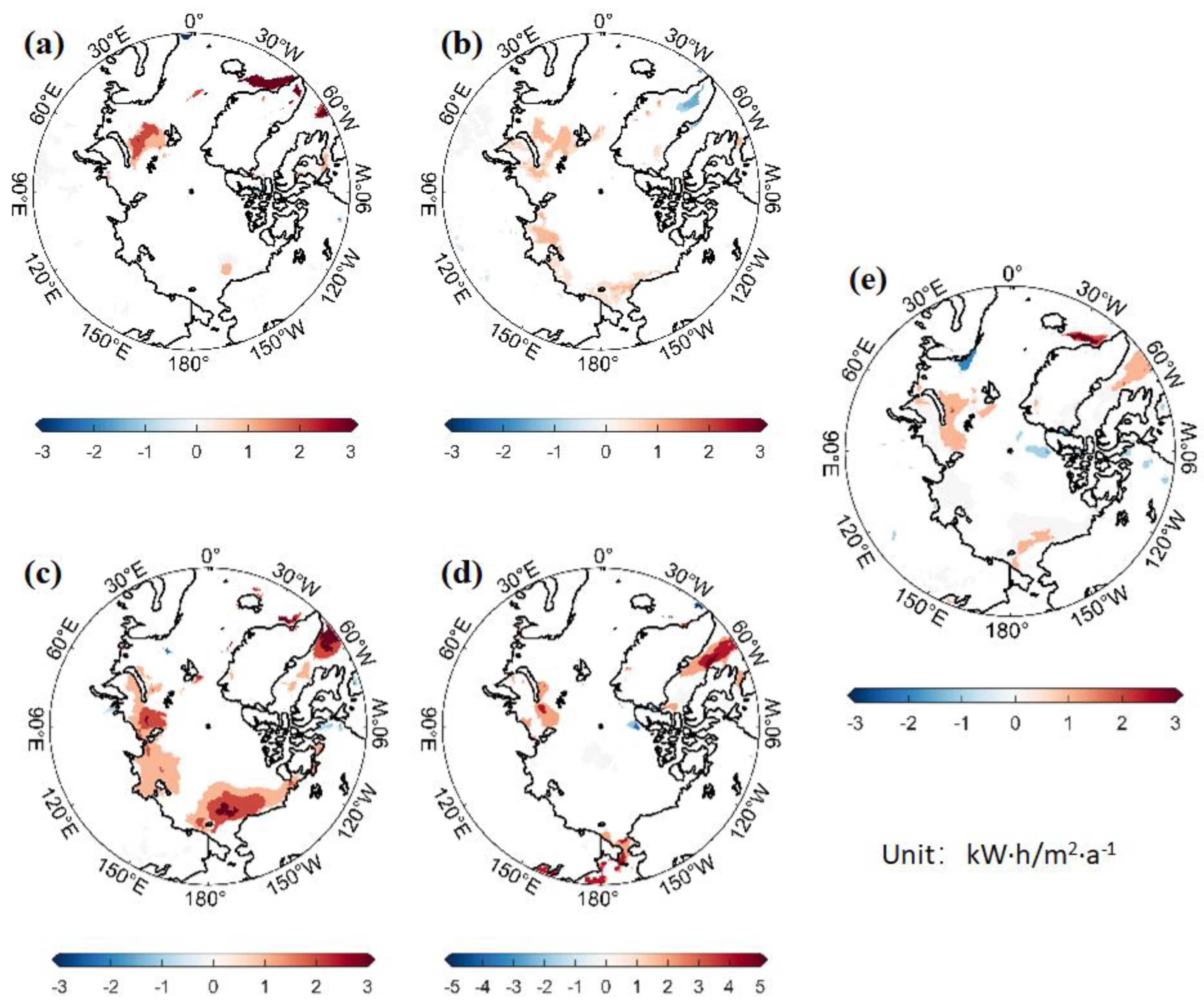
Effective reserves of wind energy resources: The trend of changes in effective wind energy reserves is consistent with that of total reserves. However, there has been a significant decrease in the negative trend in Siberia, Barents Sea, and Northern Canada waters. In spring, positive trends have expanded in the Barents Sea while strengthening in Greenland. In summer, effective reserves disappear in Siberian decreasing areas, while Greenland’s negative areas shrink, while positive areas maintain a consistent trend with total reserves. Autumn brings a positive trend to the Arctic, with negative areas almost disappearing. Typical areas include Chukchi Sea (1~3 kW·h/m²·yr⁻¹), Laptev Sea and Baffin Bay (1 kW·h/m²·yr⁻¹), Kara Sea (1~2 kW·h/m²·yr⁻¹), and Davis Strait (2~3 kW·h/m²·yr⁻¹). In winter, positive trends are found in Davis Strait, Baffin Bay (3~5 kW·h/m²·yr⁻¹), near Novaya Zemlya (1~2 kW·h/m²·yr⁻¹), and near the Bering Sea (3 kW·h/m²·yr⁻¹).

By examining seasonal variations, it is evident that the Arctic experiences a peak in effective reserves during autumn, displaying a pronounced positive trend. This favorable trend is advantageous for wind energy development and utilization.

4. Discussion and Conclusions

This study utilizes Theil–Sen Median slope estimation and Mann–Kendall trend analysis, incorporating nearly four decades of wind energy data to investigate the decadal shifts in a variety of crucial indicators for Arctic wind power.

This study suffers from the following shortcomings: the lack of Arctic observational data, which is analyzed using a reanalysis dataset; insufficiently in-depth study of the mechanisms underlying the evolutionary trend of Arctic wind speeds; and the lack of a reasonable plan for the future use of wind energy in the polar regions.

Due to the greenhouse effect, the polar atmospheric circulation is enhanced, and sea surface temperature increases. Wind speed is positively correlated with sea surface temperature, and the Arctic inland sea shows a significant increasing trend. The results indicate that:

(1) Wind power density: The Arctic’s wind power density changes are primarily influenced by autumn, with active regions concentrated in the Chukchi Sea, Laptev Sea, Davis Strait, and other locations. During spring and summer, there is a notable decline in Greenland’s area, which does not occur in other seasons. Spring sees the largest amplitude of change.

(2) Effective wind speed occurrence: The annual variation in the occurrence rate of effective wind speed is mostly influenced by autumn but with a relatively smaller magnitude. The decline area in the northern part of Baffin Island is mainly observed during spring. Positive areas are typically found near Chukchi Sea, Novaya Zemlya, Laptev Sea, and Baffin Bay, while the decreasing area spreads across the northern part of Greenland and Northern Canada’s islands. During spring, typical change areas near Novaya Zemlya and northern Baffin Island are consistent throughout the year. In summer, there is a decrease in the area near Greenland. Autumn brings about the strongest increasing trend for the Chukchi Sea and the Laptev Sea. In winter, there is no significant change in the Arctic. Baffin Bay shows a positive trend, while Siberia experiences a negative trend.

(3) Energy Level Occurrence: The change patterns of the ALO, RLO, and SLO levels in the Arctic region are similar, with a predominantly positive trend observed in Chukchi Sea, Laptev Sea, Kara Sea, near Novaya Zemlya, Davis Strait, and close to Greenland. The negative trend is mainly observed in the Barents Sea, northern Greenland, and Northern Canada. The seasonal variations of each energy level are also relatively consistent, without any significant differences.

(4) Stability: The Arctic C_v shows a predominantly negative trend, mainly observed in the Kara Sea, close to Greenland, Northern Canada Islands, and other locations. During spring, there is no notable change in the region. However, in summer, there is a positive trend in the Davis Strait, while a negative trend is observed in Greenland. The autumn and winter seasons are characterized by a significant decreasing trend, which is beneficial for wind energy stability.

The decreasing trend of M_v and S_v is consistent in the Western European Plain and the Barents Sea, with scattered significant increasing regions of S_v in Siberia, Bering Sea, northern Kara Sea, Greenland, and other places. The positive trend indicates that the difference in wind energy within the year has increased, making wind energy unstable and not conducive to its development.

(5) Resource reserves: The Arctic wind energy reserves have remained stable, with the annual trend being dominated by autumn. The positive trend is observed in the Chukchi Sea, near Novaya Zemlya, Greenland, and Davis Strait, while the negative trend is seen near the Barents Sea and Northern Canada Islands. There is no significant change in spring, but an increasing trend is observed along the northeast waterway in summer, while a negative trend is observed near Greenland. Autumn trends are consistent throughout the year but are stronger. In winter, the Arctic Sea remains unchanged, while Siberia and Northern Canada’s northern islands show a negative trend that hinders wind energy development.

Effective reserves show a predominantly positive trend, with concentrations mainly in the Chukchi Sea, Kara Sea, Novaya Zemlya, Davis Strait, and Greenland. The Northeast Passage is experiencing a notable positive shift. However, there are negative trends observed in northern Norway and close proximity to the northern islands of Northern Canada.