1. Introduction
Inside a closed system such as a power grid, all the power injected should be equivalent to the power withdrawn at each timestep, avoiding undesired events such as line congestion or blackouts. In regions where an energy market is set up, negotiations occur so that each market party commits to deliver or withdraw a certain amount of energy in the future, with penalties being applied in case of non-respect of contracts. In this way, the grid equilibrium is encouraged as each party naturally endeavors to respect the constraints, seeking to maximize their gains.
From the point of view of the producers of intermittent energy, it is thus essential to be capable of predicting their production reliably, reducing the chances of future imbalances related to taken contracts. However, because the atmosphere is inherently complex, weather-dependent power production forecasts contain a degree of uncertainty, which in many cases cannot be described by one unique point forecast. A probabilistic forecast can be helpful in such cases, defining the uncertainty through densities, quantiles, intervals, or scenarios at each timestep.
Density-based forecasts give complete information about future power generation by estimating the stochastic variable’s joint probability density function throughout the horizon. Recently, Normalizing flows were proposed for density estimation based on transforming a base probability distribution (e.g., a standard normal) into a more complex distribution by a sequence of invertible and differentiable mappings. Multiple advances have been presented in the literature since Dinh et al. first proposed using normalizing flows for density estimation [
1]. The authors in [
2] used masked autoregressive models as a form of normalizing flow, providing an easier computation of each transformation and improving the flow expressiveness by stacking multiple steps of transformations. In [
3], the authors proposed an autoregressive flow more convenient to density estimation, by using previous values sampled from the empirical distribution to generate new values (rather than previous values sampled from the base distribution, as proposed in [
2]). This modification allows the density of any data point to be estimated in one pass through the model, with the drawback of having a sequential synthetic data generation process. In [
4], an integration-based transformation flow (instead of affine transformations proposed previously) was carried out with monotonically constrained neural networks conditioned to the outputs of an autoregressive model. The proposed transformation allows more complex distributions to be estimated with fewer steps within the flow. Finally, the authors in [
5] proposed the same flow with a more computationally efficient neural network to perform integration-based transformations, whose only constraint is the positiveness of its outputs.
In quantile forecasting, the forecast determines quantiles that ensure, with a certain level of confidence, that the value is expected to be less than the quantiles predicted with the respective probabilities in the future. Quantile regression random forest (QRRF) was used as a distribution-free method for solar forecasting in [
6], as well as for the GEFcom 2014 in [
7], giving promising results; however, without comparing them with results from other recent models. The authors in [
8] compared QRRF with different models for the probabilistic forecasting of solar irradiance, verifying better methods for this application. In [
9], QRRF obtained better results compared to a quantile gradient-enhanced regression tree for a short-term load forecasting task. The authors also proposed an enhanced version where QRRF is used on top of a multi-model point forecasting pipeline, generating even better probabilistic forecasts.
Interval forecasts can better depict uncertainties with a nominal coverage rate and lower/upper bounds, such as the probability of PV production being higher/lower than a specific threshold. The lower upper bound estimation (LUBE) method, first presented in [
10], is an interval-based method that directly estimates the lower and upper bounds of prediction intervals for each timestep. This is achieved by using a loss function that optimizes the two relevant properties of prediction intervals: interval width and observation coverage. The original loss function was improved throughout the years to enable a gradient-descent-based training, as proposed in [
11] and later in [
12], with modifications to ensure a more stable training when applied to wind speed interval forecasting.
Scenario-based probabilistic models produce equally likely samples of multivariate predictive densities for the predicted variable. Generative models such as generative adversarial networks (GANs) have been highly used in the recent literature, relying on neural networks to generate sequences with random values sampled from latent space. A conditional GAN with Wasserstein distance (CWGAN) and weight clipping, instead of the original Jensen–Shannon divergence, was proposed in [
13] to generate day-ahead wind and PV power production scenarios based on labels describing day-ahead production patterns. For solar irradiance sequence generation, the authors in [
14] tested WGAN with weight clipping and gradient penalty (WGAN-GP), two ways of enforcing the Lipschitz continuity of the loss function, ensuring more stable training. The results show the superiority of WGAN-GP in generating sequences with a higher diversity and closer to the original sequences. The authors in [
15] propose a conditional WGAN-GP (CWGAN-GP) to generate load scenarios based on historical loads, day-ahead temperatures, and the day type, showing that CWGAN-GP with shallow modules can fit small datasets. A similar idea was proposed in [
16], with modules following the DCGAN-inspired configuration used in [
13] to generate wind power scenarios conditioned on labels previously predicted by a support vector regression (SVR) model using day-ahead point forecasts of wind power. Finally, wind power scenarios are generated in [
17] using an improved WGAN-GP-CT with a consistency term to enforce the Lipschitz continuity based not only on sampled data points, as when calculating the gradient penalty, but also on a region around real data points. A comparison against WGAN-GP shows that the consistency term slightly improves the stability and convergence during training and reduces overfitting when fitting on a small dataset.
The forecasts of power production obtained with the models described are generally considered inside decision-making models before market negotiations, so producers can issue energy bids for each lead time in the future, adapting their offers according to the market prices (equally predicted or fixed, as in the case of feed-in-tariff mechanisms) in a way to maximize their profits during the entire forecast horizon.
Even though the value of probabilistic forecasts has been progressively recognized within the past decade [
18], there are remaining questions about when probabilistic methods become influential in the optimal scheduling of power plants. For instance, Rahimi et al. [
19] demonstrated that deterministic forecasts achieved the second-best net profit for a 1-day optimal scheduling of a virtual power plant, surpassing three cases carried out with probabilistic forecasts. Similarly, Tostado-Véliz et al. [
20] found that deterministic forecasts yielded the lowest costs and curtailment levels when scheduling a distribution network incorporating wind power, converters, and storage. Liu et al. [
21] investigated a virtual power plant composed of multiple intermittent sources of electricity production and demand and concluded that profits were higher when using deterministic forecasts. Wang et al. [
22] conducted a study on the annual scheduling of energy production and consumption for a large-scale prosumer in the U.S., and their findings indicated that deterministic forecasts provided the lowest costs. Appino et al. [
23] focused on scheduling energy production and consumption for a household equipped with a rooftop PV power system and domestic batteries. They observed that, despite generating more significant imbalances, deterministic forecasts resulted in the lowest operating costs. Castronuovo et al. [
24] proposed an integrated approach for optimal day-ahead scheduling and real-time control of a wind power plant coupled to a pump-storage system. A 6-month analysis showed that the operation with point forecasts obtained higher overall profits than using probabilistic forecasts, tested with different nominal coverages. Ghahramani et al. [
25] examined the energy management of a distribution system comprising diesel generator units, wind turbines, storage, large industrial loads, and demand response aggregators, showing that deterministic approaches yielded the lowest operational costs in three out of four cases tested.
It is important to note that such studies were based on probabilistic forecasts generated using relatively simple methods, such as quantile regression [
23], fixed intervals [
20,
21], sampling from beta distribution [
19], and methods with incomplete descriptions [
22,
24,
25]. Other studies advocate for the clear and overall better performance of probabilistic forecasts when applied in a power plant or microgrid scheduling, considering the value of stochastic solution [
26,
27,
28]. However, this measure, traditionally used to estimate the benefits of introducing the stochastic approach, is controversial. It determines the added value by comparing the expected benefits the approaches achieve when the observations precisely follow the scenarios used to approximate the predictive distribution. However, these scenarios might not necessarily define the true underlying distribution, and different results would have been obtained if profits were calculated after applying the decisions to the actual observations.
This study aims to provide a comprehensive assessment to address these limitations and evaluate the advantages of using state-of-the-art probabilistic forecasting methods proposed in the literature. It seeks to answer questions such as whether accurate deterministic forecasts can lead to better scheduling of a PV power plant compared to probabilistic forecasts, which might tend to produce overly conservative decisions. Additionally, the study aims to explore whether the value of probabilistic forecasts increases as the underlying uncertainty grows. Furthermore, the study investigates whether probabilistic forecasts can offer more information and lead to more profitable contracts in situations where the system includes batteries to mitigate potential forecast errors, which are not accounted for by deterministic forecasts.
Performances obtained by a decision model fed with deterministic and probabilistic PV power forecasts in different situations are compared in this study. One state-of-the-art probabilistic model from each category is used in the comparison, trained with, and compared to deterministic forecasts under different accuracy levels for situations where a PV power plant produces alone or in conjunction with batteries. It is shown that the uncertainty level naturally affects overall performance, and probabilistic forecasts can effectively leverage battery capacity to manage potential forecast errors, resulting in increased profits when such assets are integrated into the system. Nevertheless, even when very inaccurate deterministic forecasts are used, the overall profits are consistently higher than average profits obtained by probabilistic forecasts in all cases. This discrepancy can primarily be attributed to the scenario diversity inherent in probabilistic forecasts, which often leads to overly conservative decisions and decisions that are not temporally correlated with PV power production variations, resulting in increased imbalances and corresponding penalties.
Section 2 describes the probabilistic models used in the study, followed by a presentation of the decision-making tool employed for optimal PV power plant scheduling in
Section 3. The study case and the data used in the modeling are provided in
Section 4. The scheduling results obtained using each forecast type are assessed and discussed in
Section 5, along with the overall financial return for each tested case. Finally, the conclusions are presented in
Section 6.
2. Probabilistic Models
The probabilistic models compared are introduced in this section, namely, normalizing flows (NFs), conditional Wasserstein generative adversarial networks with gradient penalty (CWGAN-GP), quantile regression random forest (QRRF), and lower upper bound estimation (LUBE).
2.1. Normalizing Flows
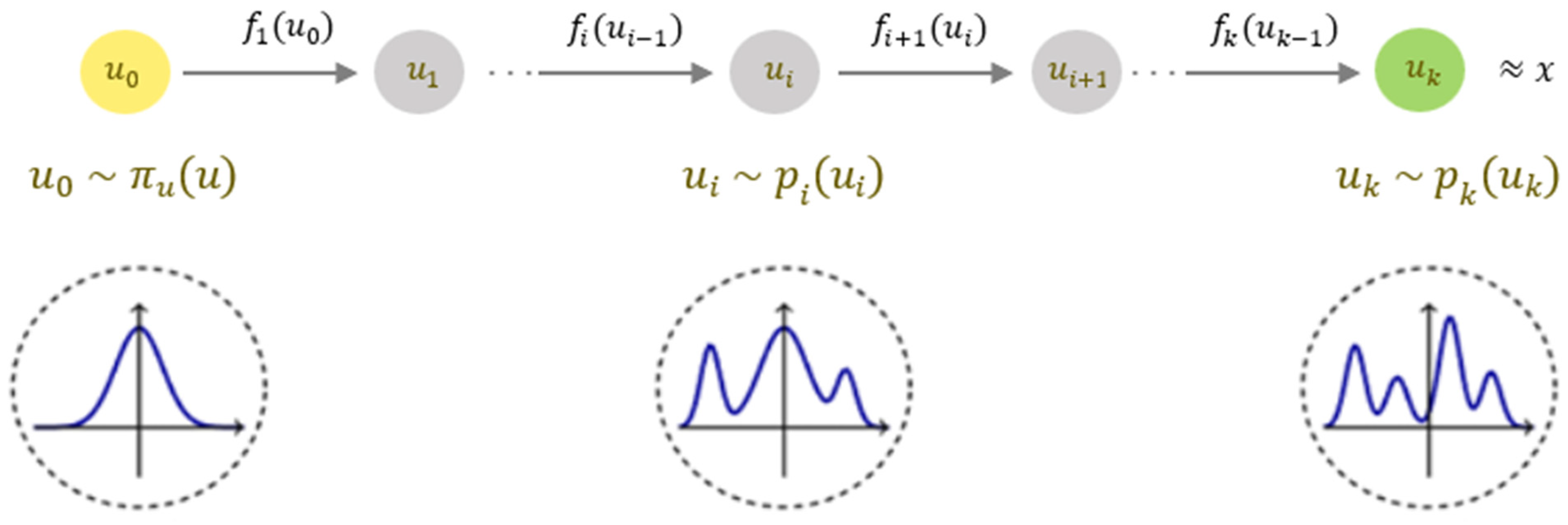
A normalizing flow consists of a series of consecutive invertible functions
, used to create invertible mappings
=
. These functions can be used sequentially to estimate densities, using
to map a complex empirical density
into a base density
, chosen such that it can be easily evaluated for any input
(e.g., a standard Gaussian, as shown in
Figure 1). Assuming the flow invertibility, the density
can be estimated as:
Using Equation (1), instead of computing each individual mapping sequentially, it becomes possible to directly calculate the entire mapping using the simplified input and the determinant of , which defines the Jacobian of regarding .
By relying on autoregressive transformations, Kingma et al. [
2] show that the Jacobian of
is triangular by design, and its absolute determinant after the consecutive
th transformation can be easily obtained as follows:
where
is a scalar function that incorporates the autoregressive property as conditionals.
Recent approaches use these properties to improve the training performance of fitting the parameters of invertible functions. One of the most recent approaches [
5] proposes using monotonic neural networks as invertible functions
, conditioned to another autoregressive model
responsible for adding information about the previous occurrences into the mapping of each data point within each transformation, for example, to model the influence of each previous timestep into current lead-time mapping throughout the prediction horizon. Such invertible functions can be calculated based on integrals:
where
is the integrand neural network with a strictly positive scalar output,
the outputs of the autoregressive conditioner, and
a neural network with a scalar output. Integral-based transformations provide a much more effective transformation compared to affine or non-affine transformations, requiring a reduced number of consecutive functions to perform superior mappings. The authors in [
5] proposed solving the integral (3) more efficiently by approximating it numerically using the Clenshaw–Curtis quadrature.
In this case, the autoregressive conditioners are also defined by neural networks, based on the masked autoregressive network (MAF) proposed in [
3], which relies on blocks of masked autoencoders for distribution estimation (MADE), previously proposed in [
29], to parameterize each autoregressive embedding
of the flow simultaneously.
Integral-based transformations, combined with masked autoregressive conditionals, provide an effective and efficient flow, giving promising results compared to other probabilistic models [
30]. The same architecture was used in this study, with adaptations only in the input layers of the autoregressive conditioners, fed with previous lead times of the prediction horizon for each occurrence. Moreover, even if normalizing flows can perform density estimation, only values sampled from the final predictive joint density were used in this study, defining PV power scenarios for each day.
2.2. Conditonal Wasserstein Generative Adversarial Network with Gradient Penalty (CWGAN-GP)
CWGAN-GP consists of two adversarial modules, a generator and a critic. The generator maps random numbers and conditional values to scenarios of PV production. The random values, sampled from a distribution (often Gaussian or uniform), define the variations of each scenario representing the forecast uncertainty, and deterministic PV power forecasts used as conditionals guide the generator to produce realistic sequences. On the other side, the critic receives sequences of PV production (synthetic or real sequences) with the same conditionals and outputs a score defining the authenticity of each sequence.
Figure 2 depicts the general structure of the CWGAN-GP model:
During training, the generator tries to produce synthetic sequences following the distribution of real sequences conditioned on the deterministic forecasts; the critic receives synthetic (generated) or real sequences along with conditionals, outputting a score to each sequence. This score will be lower for sequences looking synthetic and higher for convincing sequences. At each iteration, both modules improve based on the difference between the critic score and the actual score of each sequence; the generator becomes better at generating realistic-looking sequences each time, and the critic becomes better at discriminating synthetic sequences from real sequences. When all scores yielded by the critic converge to a small value, the generator is trained enough and able to produce new realistic scenarios.
In a general form, the objective functions are described as follows for each module:
The generator seeks to increase the score the critic gives to its generated sequences
. In contrast, the critic seeks to maximize the difference between the scores given to real data and synthetic data
. Therefore, the adversarial game between these two modules can be presented as a min–max optimization model:
To ensure a stable training for the critic, recent studies adopted a gradient penalty applied to the critic’s objective function. This gradient penalty conducts the objective function as 1-Lipschitz, limiting the norm of its gradients to at most one everywhere. The gradient penalty is given by:
where
is a random weighted average between generated and real samples, estimating points close to such sequences within the search space.
denotes the expected value over all the weighted samples;
is a hyperparameter used to determine the weight of the gradient penalty in the loss function. The critic’s final objective function can be defined as:
In this study, both generator and critic are autoregressive, composed of temporal convolutional networks (TCN), proven to be more accurate, capable of retaining longer sequences, and more efficient to train than recurrent networks [
31]. The difference between the two modules is that the receptive field of the critic should be bigger to account for and evaluate the entire sequence, whereas the generator’s receptive field should be long enough only to account for lagged correlations of each timestep. In addition, the generator outputs the whole generated sequence, whereas the critic outputs a single score. Furthermore, for each generator iteration during training, the critic is trained five times in this study, as its structure is more complex than its adversary’s. The model will be called WGAN for conciseness purposes.
2.3. Quantile Regression Random Forest (QRRF)
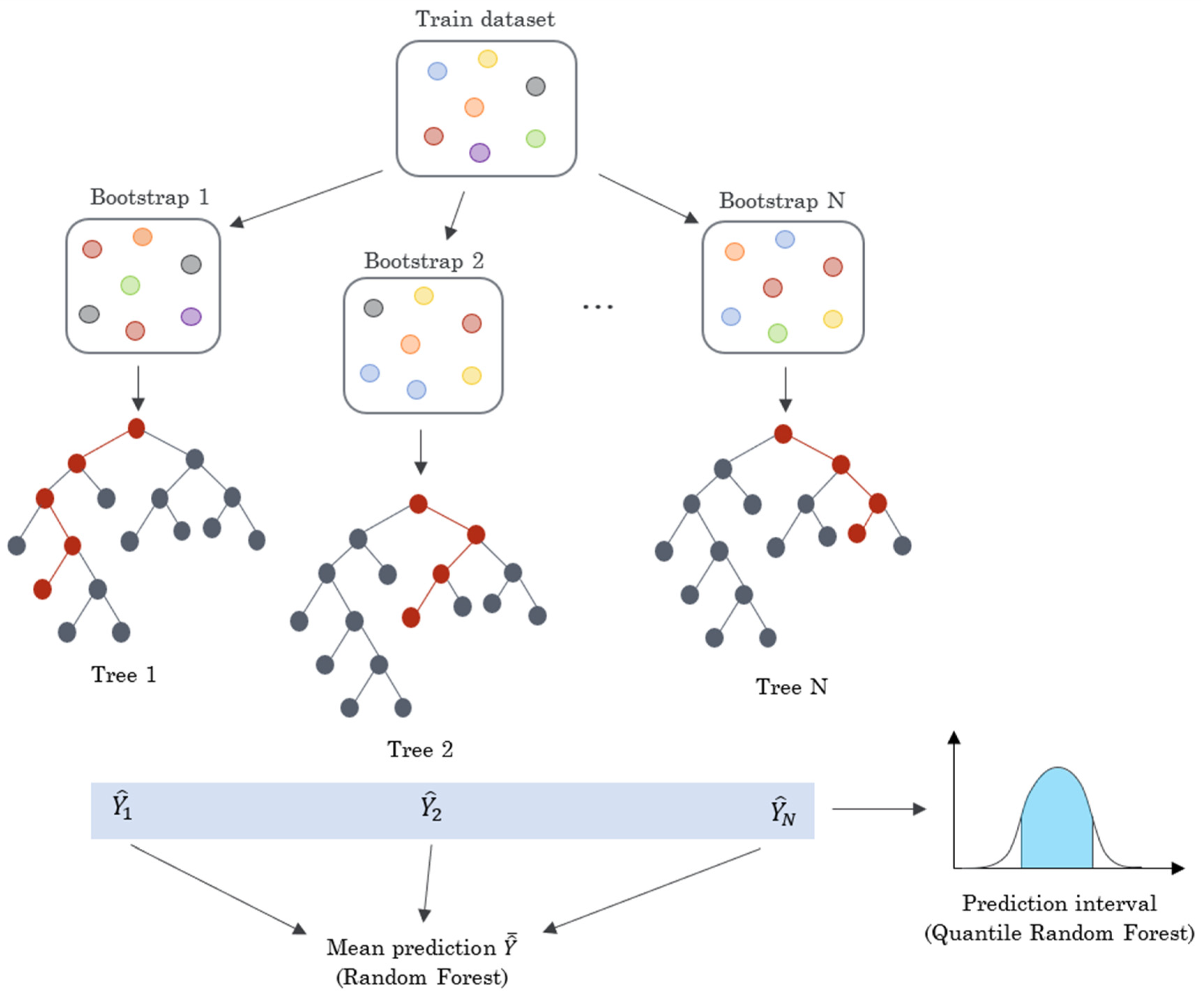
QRRF is a tree-based ensemble method for estimation of conditional quantiles. It applies quantile regression on top of the random forest algorithm, building an effective and widely used learning model based on decision trees to model the prediction uncertainty that random forests cannot represent alone.
Unlike random forests, which focus on the average of predicted values from leaf nodes, QRRFs preserve all values within each leaf node, providing the complete conditional distribution of each prediction [
9]. The quantile regression part of the algorithm is used to output quantiles of the resulting conditional distribution for each forecast lead time.
First, a random forest is constructed using an ensemble of decision trees. Each tree is trained on a bootstrap sample of the original training data, where each tree is exposed to a random subset of the features. The construction process involves recursively splitting the data based on the feature values to minimize the variance in the target variable within each leaf node. This iterative splitting process forms the hierarchical structure of the decision tree, with each internal node representing a decision based on a feature and each leaf node representing a predicted value.
Once all the decision trees are constructed, predictions are made by aggregating the predictions of each tree. In the case of regression tasks, a common aggregation method is to average the predictions of all the trees. This ensemble approach helps to mitigate each tree’s biases and provides a more robust prediction.
Figure 3 shows the “quantile component” of QRRF models, implemented only in the prediction phase, when the outputs from each tree are used to construct the prediction interval using different quantiles. This approach offers the advantage of predicting multiple quantiles simultaneously, eliminating the need for model re-training and increasing the workflow speed.
The quantiles predicted using QRRF are converted into predictive distributions by interconnecting the quantiles predicted at each lead time using a smooth function. However, the downstream decision-making method used to schedule the PV power plant in this study needs scenarios of PV power production as inputs. Therefore, an additional method, called ensemble copula coupling (ECC), was used to build scenarios based on the predictive distributions.
First proposed in [
32], the ECC procedure is defined as follows for each QRRF forecast:
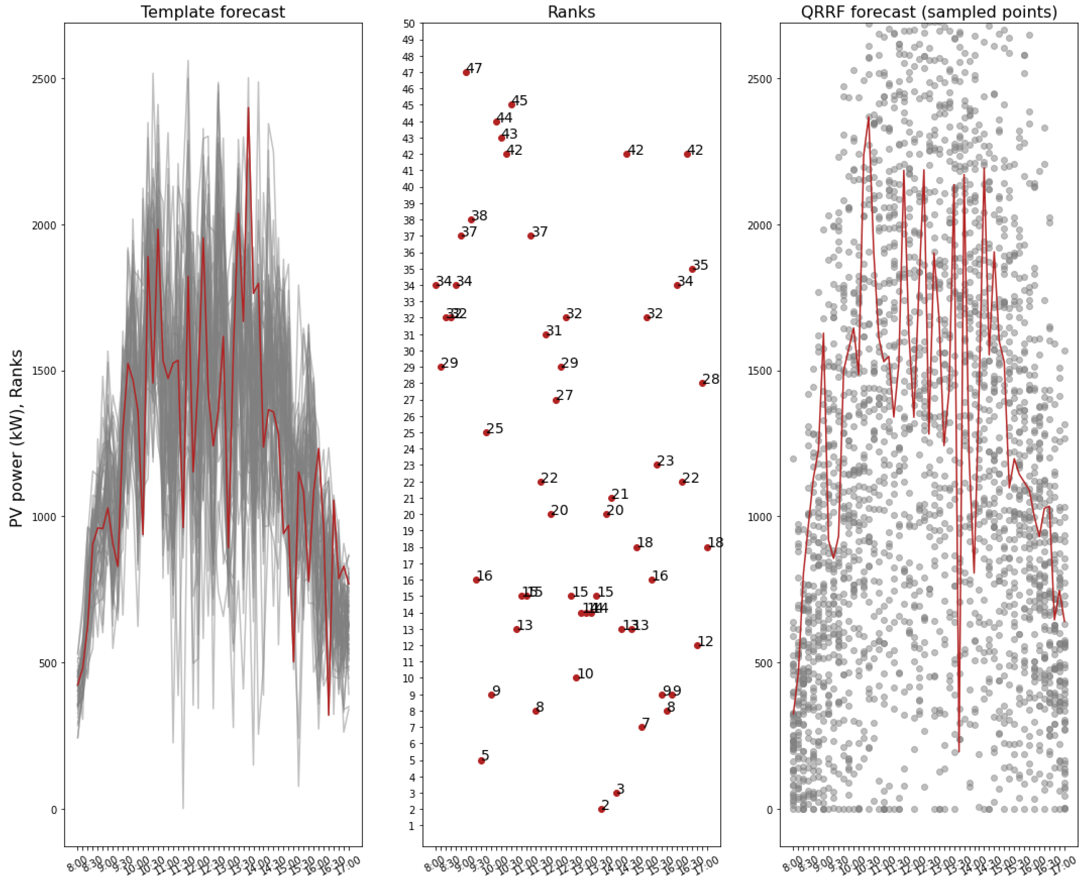
Using another scenario-based probabilistic forecast issued for the same day as a template, extract the rank matrix defining how values from one lead time are connected to values from subsequent lead times.
Sample values from normal distributions defined with the bounds of the predictive interval at each lead time.
Rearrange the sampled values with the same rank extracted from the template in 1.
The procedure is depicted for the reconstruction of one scenario in
Figure 4.
Finally, the QRRF reconstructed scenarios have the same correlation between lead times as observed between lead times of probabilistic forecasts used as the template.
In this study, the QRRF model was trained using the scikit-garden library available in Python. Probabilistic forecasts previously obtained with WGAN were used as templates for generating QRRF scenarios, as the former produces scenarios with correlations most similar to those present in observations (not shown).
2.4. Lower Upper Bound Estimation (LUBE)
The original LUBE model, first proposed in [
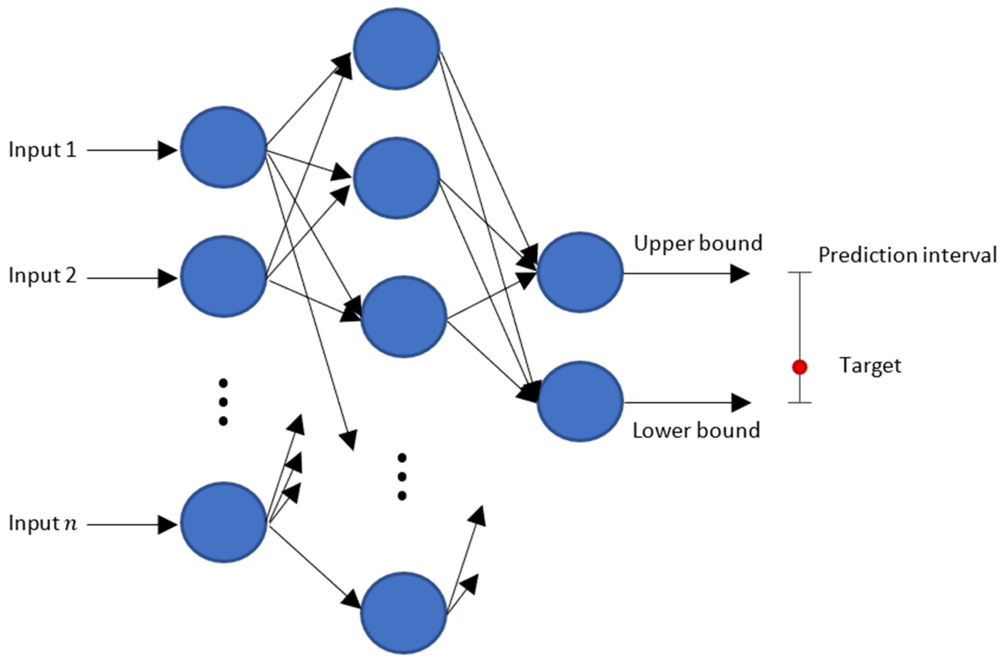
10], is an interval forecasting method using a typical artificial neural network with two neurons in the output layer: one for the upper-bound prediction and the other one for the lower-bound prediction.
Figure 5 shows the general structure with two outputs defining the prediction interval (PI).
The advances in the method focused mainly on the loss function, trying to define a suitable, continuous, and differential objective function for gradient-descent-based training. In this study, the objective function proposed in [
11] was used, which is a combination of two loss functions, namely, prediction interval coverage probability (PICP) and mean prediction interval width (MPIW) of covered points:
where
defines the total number of data points covered by the PIs and
the total number of data points. High-quality PIs should be as narrow as possible, while capturing some specified proportion of data points [
11]. Therefore, an efficient training should seek to minimize
, subject to
, where
is a significance level. After some algebra, the final objective function is defined as:
where
controls the importance of width versus coverage. In the original paper, a final adaptation was made in the computation of
, using a sigmoid function to create a smoother and more differentiable step function, defined by
:
In this study, the LUBE model comprises a multi-layer perceptron with two hidden layers. The best combination of hyperparameters for each data frame was obtained using the grid search and particle swarm optimisation algorithms.
After generating the predicted intervals, the scenarios to be used in the decision-making model were built using the ECC method, as for QRRF forecasts.
3. Downstream Decision-Making Model
Two-stage stochastic programming was chosen as a decision-making model to optimize the functioning of the PV power plant based on the forecasts covering a prediction horizon. The model seeks to maximize the daily profits by injecting energy when prices are high and storing energy when prices are low, as well as compensating the imbalances given by the difference between the declared and actual PV power production, avoiding corresponding penalties.
The underlying decisions are divided in two stages: first-stage decisions are defined “here and now” and taken promptly at each timestep, followed by the resolution of the uncertain variable defined by the PV power production. Second-stage decisions, also called recourse decisions, are taken “wait and see” as corrective actions after the realization of the random variable [
33]. The process is depicted in
Figure 6 for a single timestep and for the entire horizon.
First-stage decisions, in our case, represent the declared power to be injected at each timestep throughout the day. Conversely, the second-stage decisions are defined by the power withdrawn from the grid, the power curtailed, and the battery power, which will be used to absorb forecast errors after the realization of the PV power production, seeking to reduce the difference between the declared power to be injected and the actual injected power. Incidentally, the battery power will also participate in the first stage, along with the PV power expected to be produced and directly injected into the grid, to propose the most advantageous contract for future power injection.
Translating the two-stage stochastic programming into a mixed integer linear program (MILP) makes it possible to build an objective function submitted to constraints easily solved by ad hoc solvers:
Submitted to constraints:
The objective Function (14) defines the maximization of the overall profits, composed of the power declared to be injected as a first-stage decision paid at a price , minus the positive imbalances sanctioned at a price , minus the negative imbalances sanctioned at a price . The imbalances may occur when the producer cannot deliver the power declared after the PV production and BESS power decisions are realized. The calculations are performed for each timestep and scenario , where each scenario has a probability .
The constraints applied to the objective function define the feasible region imposed on the decisions of the problem. Firstly, the declared power , is limited by the maximum power allowed to be withdrawn from the grid and by the maximum expected PV power production plus the nominal battery discharge power (15). The power injected for each scenario is defined in (16) as the forecast PV power minus the net battery power, minus the curtailed power, minus the power to be withdrawn from the grid used to recharge the batteries. In (17), the imbalance is defined as the difference between the injected power for each scenario and the declared power, and in (18) the imbalance is decomposed into positive and negative imbalances, which will be constrained in the subsequent Equations (19) and (20), respectively. The binary variable helps to set to zero the negative imbalance if there is a positive imbalance or vice versa. Equation (21) defines the batteries’ state of charge evolution according to the charge and discharge power. The storage capacity, charge, and discharge power limits are defined from (22) to (24). The limits for the power to be curtailed are defined in (25). The maximum allowed ramps for the power declared are defined in (26) and for the battery in (27).
The outputs of this decision-making model are the power declared to be injected at each timestep, along with the charge and discharge battery power, the power to be curtailed, the power to be withdrawn from the grid, and the state of charge of the batteries for each timestep and scenario throughout the horizon. The profits for each day are then calculated by applying such decisions with the actual PV power produced during the day, respecting the physical constraints of the problem: for example, not curtailing or charging more power than the power produced at each timestep, or not exceeding the maximum or minimum limits of the battery. For the application of second-stage scenario-dependent decisions, i.e., all decisions besides the declared power, the expectation of all scenarios was considered for each timestep.
The electricity prices are known in advance in a feed-in-tariff mechanism, and considered to be constant during the day, so the added value when working with batteries is primarily due to the ability to reduce imbalances, rather than to perform shifting or arbitrage. The penalties for negative imbalances are set two times higher than penalties caused by positive imbalances. Other parameters, such as maximum PV power, maximum battery power and capacity, maximum allowed power to buy, and maximum and minimum allowed ramps, are defined in
Table 1 and are set equally for all cases. The calculations were implemented using the CPLEX solver, with the pyomo library available in Python.
4. Study Case
This study focuses on the procedure adopted by any producer of intermittent energy who seeks to sell their production in an optimized way, either by bidding on a wholesale market or declaring the energy that will be injected during the day to the transmission operator in a feed-in-tariff mechanism. Regardless of the final beneficiary, the producer is always submitted to constraints and penalties, making the generation of accurate forecasts essential.
To exemplify this procedure, a PV power plant with batteries was selected in French Guiana, a location where the climate conditions provide atmospheric instability and higher degrees of PV production uncertainty. The power plant has 3.8 MW of installed capacity and is connected to 2.9 MW batteries reaching 2.6 MWh of storage capacity. Three years of PV power production between 2020 and 2023 was extracted with a 10 min time resolution to fit and test the models compared in this study.
The PV power deterministic forecasts were obtained by first generating weather forecasts with the Weather Research and Forecasting (WRF) numerical model during the same period and time resolution as historical PV power production. These were then converted to PV power forecasts using a multi-layer perceptron neural network, issued daily at 00:00 with a 10 min resolution for 24 h.
To investigate the performances based on deterministic forecasts with different accuracy levels, the original forecasts were averaged in a 30 min and hourly time resolution, adding bias by removing the predicted variations in PV power. This approach for adding bias was chosen as it mostly represents inaccurate PV power forecasts used to predict high temporal resolution production. Another dataset of deterministic forecasts was obtained through satellite-based approaches (not shown), generating less accurate forecasts than WRF-based forecasts when predicting such an unstable climate with high temporal resolution.
Figure 7 shows the random and systematic errors of each dataset, measured using the normalized mean absolute error (nMAE) and the mean bias error (MBE), respectively:
The deterministic forecasts, also used as conditionals in probabilistic models, vary from very accurate and unbiased deterministic forecasts, such as forecasts #1, to very inaccurate and highly biased deterministic forecasts, such as forecasts #4. The datasets’ names are sorted according to their degree of accuracy: original 10 min resolution forecasts (#1), resampled 30 min resolution forecasts (#2), resampled hourly resolution forecasts (#3), and satellite-based forecasts (#4).
Finally, the deterministic forecasts and PV power measurements were used to fit each probabilistic model compared in this study in a threefold cross-validation: the entire dataset was divided into three subsets comprised of one year of point forecasts and PV power observations each. Each model is trained on two of these sets combined and used to generate 100 scenarios for each day of the remaining one, which are fed into a decision-making model. For each case, this process is repeated three times, each time using a different test subset.
Table 2 depicts the main hyperparameters used in each model.
The NF training used the same hyperparameters adopted by Dumas et al. [
30]. In WGAN modeling, the blocks of temporal convolutional networks (TCNs) have been assigned dilations corresponding to the prediction horizon length, with a standard number of layers and neurons. The other hyperparameters followed the implementation in [
14]. QRRF was trained with standard hyperparameters as in the example provided in the official scikit-garden documentation [
34]. Finally, the LUBE method was implemented with standard hyperparameters adapted to the task.
5. Results and Discussion
Figure 8 shows the forecast capabilities of deterministic forecasts for a day selected randomly, according to their accuracy level. From #1 to #4, fewer PV power variations were predicted each time, gradually decreasing the accuracy.
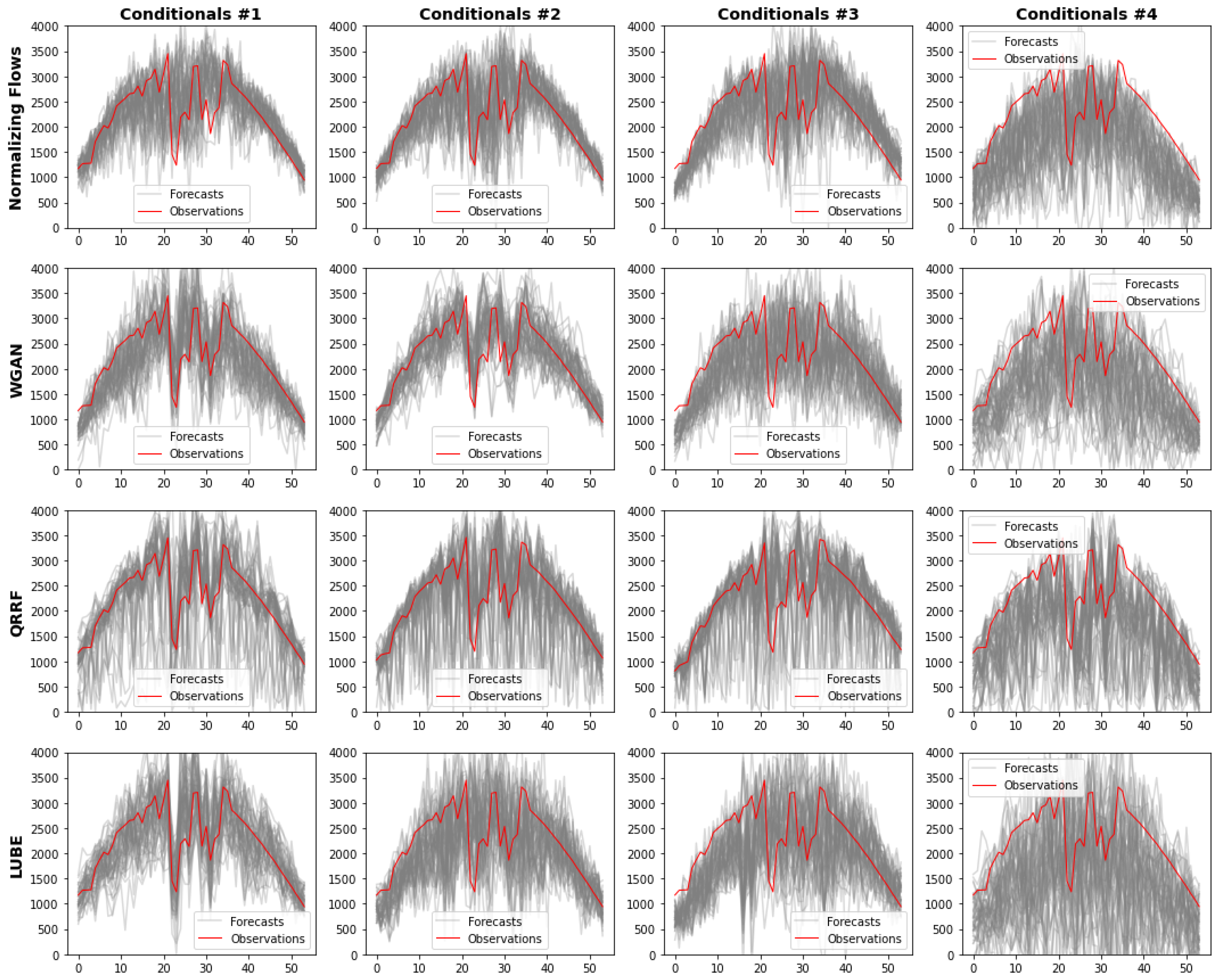
Figure 9 shows the scenarios generated by each method conditioned to the point forecasts for the same day. The spread of scenarios defines the uncertainty modeled by each method. Naturally, scenarios adopt a larger spread with the degradation in deterministic forecasts accuracy—progressively, from conditionals #1 to conditionals #4, indicating higher uncertainty levels. It is also shown that some methods capture a much more pronounced uncertainty than others; WGAN produces scenarios with the narrowest spread, followed by normalizing flows, QRRF, and LUBE, capturing the highest amount of uncertainty. Indeed, it can be seen that QRRF captures an oversized uncertainty even when conditioned to accurate conditionals (#1).
Figure 10 depicts the final profits obtained with the optimal scheduling carried out for two years for study cases with and without batteries, with each of the four deterministic forecasts used as conditionals in probabilistic models.
Firstly, it is evident that the overall profits obtained by the system decrease as the accuracy of the forecasts deteriorates. This holds true regardless of the specific forecasting model used or the incorporation of battery storage. In other words, as the forecasts become less accurate, the ability to maximize profits through optimal scheduling diminishes.
Furthermore, the results consistently demonstrate that connecting the system to batteries leads to higher profits. This is primarily attributed to the batteries’ capacity to absorb potential imbalances, thereby reducing curtailment and minimizing the loss in PV power that would otherwise occur.
The results also reveal that the profits obtained using deterministic forecasts were higher than those obtained using probabilistic forecasts generated by each model in every case. Even when very inaccurate point forecasts (#4) were used, deterministic forecasts still yielded the best profits, along with profits obtained with LUBE forecasts for the case with batteries. This discrepancy can be attributed primarily to the scenario diversity in probabilistic forecasts.
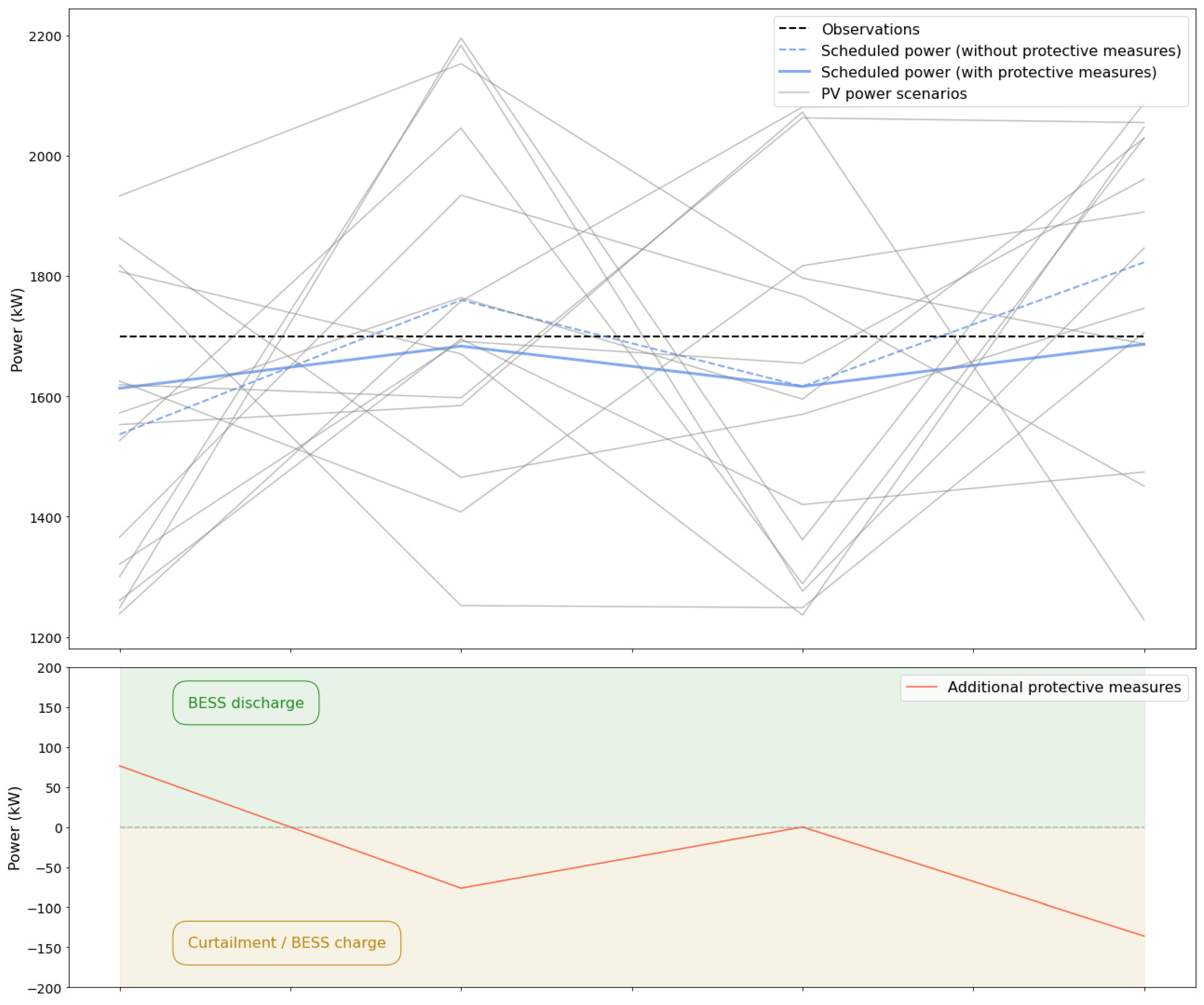
While diversity is essential in capturing the underlying uncertainty associated with each point forecast, in the context of PV power plant scheduling, it is equally important to have scenarios correlated to the observations, ideally capturing the same PV power variations. Suppose different scenarios predict diverse spikes in future PV power production. In that case, the decision-making model tends to adopt overly conservative decisions, such as reduced declared power to be injected or higher curtailment levels, protecting the system against all potential variations that may not necessarily occur. Consequently, this conservative approach leads to below-average performance and lower revenues.
Figure 11 shows a simple example of a four-timesteps period of constant PV power production, where diverse scenarios predict different PV power production variations. Naturally, the declared power to be injected has a profile corresponding to the expectation of such variations, which may violate injection requirements such as ramp limits for the power injection or additional BESS power. To mitigate such variations, protective measures such as curtailment or BESS charge/discharge were applied to smooth the declared profile, resulting in further penalties as the real PV power production is constant. Scheduling based on already smooth deterministic forecasts would not require such protective measures, as the expected PV power production would not violate ramp limits. This phenomenon is observed across all tested uncertainty levels, including cases where point forecasts are already accurate.
When utilizing deterministic forecasts, the decision-making model can establish coherent decisions based on accurate forecasts, or decisions that guarantee at least moderate productivity when point forecasts fail to predict the PV power variations, as the uncertainty level increases.
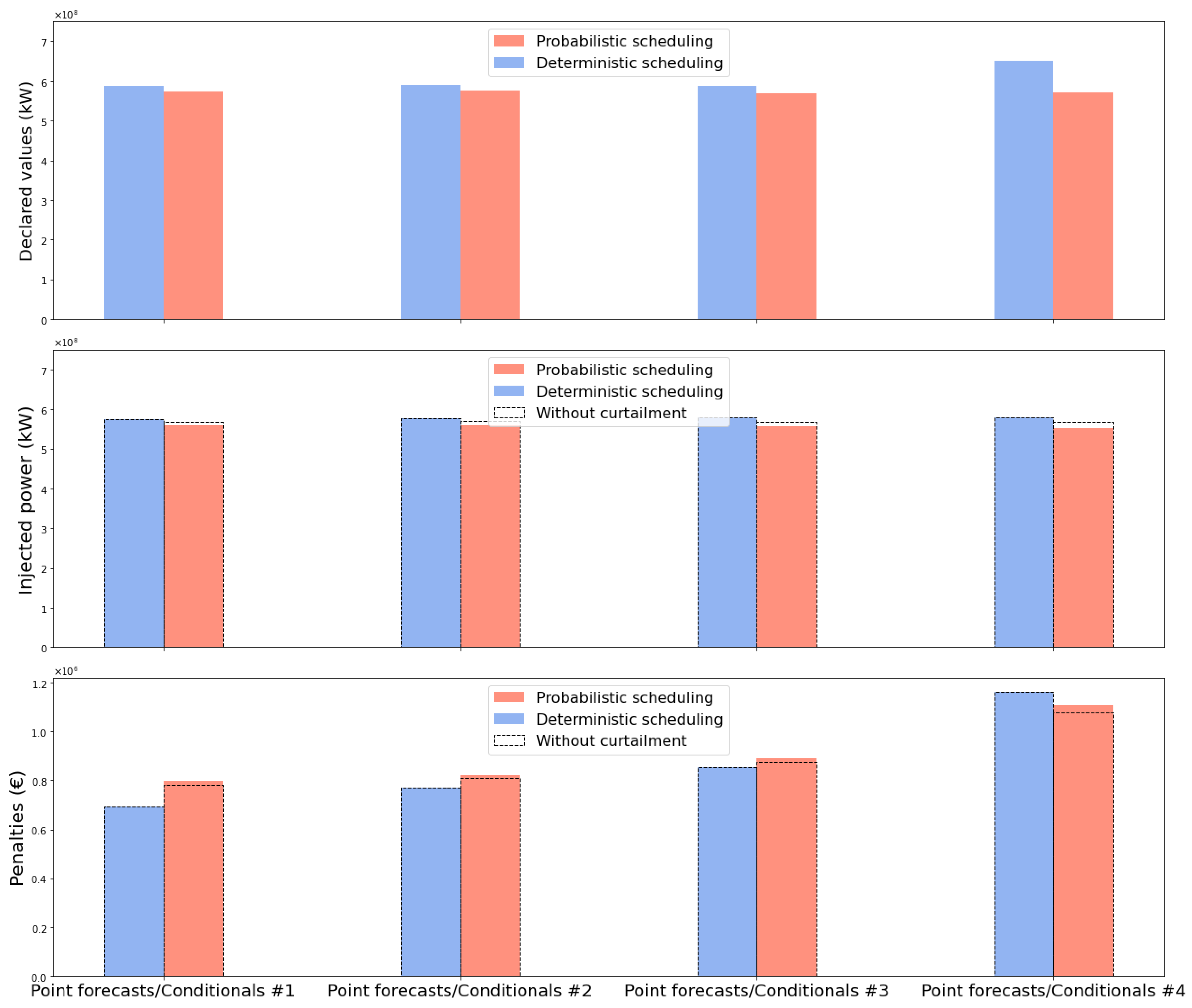
Figure 12 illustrates this behavior when the system is connected to the batteries. The scheduling using deterministic forecasts generates each time more confident and optimistic declarations, especially for forecasts #4, which tend to overestimate the PV power production, as shown previously in
Figure 7. Conversely, the probabilistic scheduling generates more conservative declarations, anticipating more power to be curtailed during the day. When such curtailments are carried out, the probabilistic scheduling suffers even higher penalties, confirming that such protective actions are not taken at the right moment because of diverging scenarios, resulting in further imbalances.
The overall profits and the value obtained for each level of uncertainty when batteries are connected to the system are reported in
Table 3, with the average added value of adopting a probabilistic approach for each case.
To illustrate the differences between probabilistic forecasts and deterministic forecasts in the scheduling of a PV power plant,
Figure 13 proposes a twofold analysis: the top portion displays the scheduling realized by the decision-making model based on the forecast PV power for a day selected randomly. The bottom part showcases the power injected after the decisions were applied and the corresponding imbalances for the same day.
On the left side of the image, we have the results obtained using probabilistic forecasts generated with normalizing flows. These forecasts accommodate the variations observed in the measured PV power quite well. However, due to the inherent spread of scenarios provided by the probabilistic forecasts, the scheduled injected power tends to be more conservative. On the right side of the image, we have the results obtained using point forecasts of PV power with a certain level of uncertainty. Unlike the probabilistic forecasts, these point forecasts only predict an average PV production without accounting for potential variations. Consequently, the scheduling based on these point forecasts tends to be more ambitious, assuming smooth and consistent PV power production.
The injected power tends to be similar in both cases, as the deterministic scheduling does not propose interfering decisions, given its confidence in the smoothness of PV power production based on its predictions, and the probabilistic approach suggests average decisions based on the expectation of the decisions that would have been taken for each scenario. Although more conservative, the probabilistic scheduling is subjected to more significant penalties, as the predictions used were not completely centered around the measured PV production, leading to more consequential imbalances.
The same assessment was conducted using measurements and point forecasts in hourly time resolution (not shown), which showed the same trends observed when observations and penalties were calculated with a 10 min time resolution. This refutes a hypothesis that a high temporal resolution would induce the over-conservative performance of probabilistic forecasts, and indicates that a producer seeking to optimize the revenues of a PV power plant can still obtain more profits by investing in accurate deterministic forecasts rather than investing in probabilistic approaches.
6. Conclusions and Perspectives
This paper aimed to comprehensively assess the advantages and limitations of using state-of-the-art probabilistic forecasting methods for the optimal scheduling of power plants compared to deterministic forecasts. The objective was to address the increasing recognition of probabilistic forecasts in recent years and to answer remaining questions about their effectiveness in power plant management. Questions include whether accurate deterministic forecasts outperform probabilistic forecasts in overall profitability, whether this trend persists with a growing system uncertainty, and whether they offer more profitable contracts when batteries are integrated into the system.
To achieve these objectives, the paper employed a stochastic programming model and compared its performance when fed with deterministic and probabilistic forecasts in various scenarios, including standalone PV power plant operation and hybrid operation with batteries. Different representative probabilistic forecasting methods were employed and evaluated against deterministic forecasts with varying levels of uncertainty. The profits were calculated after applying the expected scheduled decisions calculated daily over three years of real PV power production for each case.
The main findings indicate that while probabilistic forecasts offer potential benefits in managing uncertainty and utilizing battery assets to mitigate forecast errors, deterministic forecasts consistently yielded higher profits in almost all cases tested. This discrepancy is primarily attributed to the scenario diversity in probabilistic forecasts leading to over-conservative decisions and a lack of temporal correlation with PV power production variations. Consequently, these factors increased imbalances and penalties, impacting overall profitability.
In summary, this research contributes to understanding the practical implications of probabilistic forecasting methods for power plant management. While probabilistic forecasts have the potential to offer benefits in certain situations, deterministic forecasts currently outperform them in terms of profitability. As such, further advancements in probabilistic forecasting methodologies and techniques may be necessary to fully unlock their value in power plant scheduling.
The insights gained from this study can inform decision makers and researchers, contributing to the ongoing efforts to advance forecasting techniques for efficient and profitable power plant scheduling in the face of uncertainty. Further research could focus on rigorously validating the effectiveness of probabilistic techniques across diverse PV power plant settings and climatic conditions, bolstering the reliability and generalizability of the trends observed in this study. Additionally, exploring the added value of probabilistic approaches when more uncertain variables are added to the system could be a promising avenue for future exploration.
