Mid-Term Optimal Scheduling of Low-Head Cascaded Hydropower Stations Considering Inflow Unevenness

Abstract

China has a vast scale of hydropower, and the small hydropower stations account for a large proportion. In flood season, the excessive inflow keeps these stations at a high reservoir level, leading to a worse condition of hindered power output and a great error in the calculation of power generation. Therefore, this paper proposes a mid-term optimal scheduling model for low-head cascaded hydropower stations considering inflow unevenness, in which the power output is controlled by the expected power output curve and daily inflow–maximum power output curve. A case study of nine hydropower stations on the Guangxi power grid shows that, regardless of considering the fitted curve or not, there are different degrees of error between the planned and actual situations. However, the error and power generation are decreased when considering the fitted curve, which reflects the impact of hindered power output. Meanwhile, according to the comparison, the weekly plan is more in line with the real condition when using this model to solve the problem. The results indicate that this model improves the accuracy of power output calculation for low-head hydropower stations with uneven inflow, playing a key role in the process of scheduling.

1. Introduction

In recent years, more and more studies have focused on the mid-term optimal scheduling of hydropower stations for its comprehensive function [1]. On the one hand, it has the ability to meet the needs of the power market in time and maintain the balance between supply and demand [2]. Therefore, in power market transactions and dispatching, it can optimize the economic benefits and improve the market competitiveness of hydropower stations based on market prices and competition conditions [3]. On the other hand, mid-term scheduling considers future water inflow, seasonal changes in hydropower’s power output, and the probable trend of the power market’s development. Over a long period, it can reasonably dispatch water resources to make full use of water inflow and reduce spilled water. Thus, it appears to be significant to derive the best plan for mid-term scheduling.

For cascade hydropower stations, there are commonly three methods for addressing hydropower scheduling problems [4]—linear programming (LP), heuristic algorithms, and dynamic programming (DP)—and each method has its advantages and shortcomings. The biggest advantage of linear programming is that it is a feasible solution that is easier to derive compared with other methods [5], but the restrictions are equally obvious because this method is only suitable for the condition that the constraints and the objective function are all linear. When it comes to nonlinear problems, there is no solution using this method [6], and the other two methods appear to be functional. Heuristic algorithms, such as genetic algorithms (GA) [7], particle swarm optimization (PSO) [8], ant colony optimization (ACO) [9], and simulated annealing (SA) [10], are more suitable to solve the problem of large-scale cascaded hydropower stations on account of their powerful computing ability. However, what hinders their development is that heuristic algorithms easily prematurely converge to a locally optimal solution. As for dynamic programming [11], it is widely adopted in cascaded hydropower station scheduling. It divides a complex problem into several easier subproblems and obtains the globally optimal solution by solving the subproblems. Nevertheless, the curse of dimensionality appears as the scale of the problem increases, making it difficult to figure out a high-dimensional problem. On this issue, a great deal of improved dynamic programming algorithms [12], like progressive optimality algorithms (POA) [13,14], dynamic programming with successive approximation (DPSA) [15,16], and discrete differential dynamic programming (DDDP) [17,18], come into use. For example, Shen et al. [19] proposed a method combined with random sampling and a progressive optimality algorithm to address the problem of the curse of dimensionality caused by the large scale of cascaded hydropower stations, and the results proved that the amount of computation is greatly reduced. Li et al. [20] proposed an improved decomposition–coordination and discrete differential dynamic programming (IDC-DDDP) method to solve the problem of optimizing large-scale hydropower systems. He et al. [21] proposed an improved DPSA with a relaxation strategy (named DPSARS) based on the above mathematical derivations to solve the long-term joint power generation scheduling (LJPGS) of a large-scale hydropower station group (LHSG) and improved the calculation accuracy.

However, there is a large error for low-head hydropower stations if we derive solutions through these methods directly. Compared with high-head hydropower stations with robust adjustment ability, like the Three Gorges hydropower station, which plays a vital role in the optimal scheduling of reservoirs [22], the practical plan of low-head hydropower stations is more difficult to derive [23]. On the one hand, these low-head hydropower stations have small storage capacity, making it hard for them to change the power output in time based on inflow, especially when it comes to extreme rainfall. Meanwhile, due to the inflow being uneven every day, if we ignore the variation in inflow within a day and calculate power output with mean daily inflow, there is much error for power generation and water spillage. Although in many studies inflow unevenness is not considered—for example, Fredo et al. [24] related output with head, turbine outflow, and efficiency of the generating units to derive the operation rules in long-term optimal scheduling without considering inflow unevenness—in reality, inflow unevenness seriously affects the accuracy of optimal scheduling. Over the past 30 years, optimal scheduling considering inflow unevenness has gradually been studied. Ge et al. [25] proposed a novel stochastic optimization algorithm using Latin hypercube sampling and Cholesky decomposition combined with scenario bundling and sensitivity analysis (LC-SB-SA) to address the problem of inflow unevenness. Akbari et al. [26] integrated fuzzy-state SDP and multicriteria decision making to address inflow unevenness for a single reservoir. Zhang et al. [27] estimated the unevenness of reservoir operating rules through the Bayesian model averaging model, which combined three popular operating rules to reduce the unevenness of operating rules. Wang et al. [28] developed a hedging model for hydropower operation, which determined more rational carryover storage decisions when considering inflow unevenness. On the other hand, these low-head hydropower stations have small storage capacity, so it is possible for them to experience significant fluctuations in water level. In flood season, the inflow surges, and if the reservoir is already near or at its water level limit, measures including flood discharge and water release should be taken to control the reservoir’s water level to prevent safety issues. As a result, frequent fluctuations in water level can result in unstable generating flow, which reduces the efficiency of the turbine, and, finally, leads to hindered power output. This is why, with the increase in inflow, low-head hydropower stations’ power output increases first and then decreases. Additionally, when it comes to extreme rainfall, the tailwater level of hydropower stations continues to rise and the water head for generating becomes lower, leading to the result that power output is seriously hindered [29] and estimating low-head hydropower stations’ power output becomes more difficult. In the past, the expected output curve was used to compute power output, but the results were quite different from the actual ones for the reason that hindered power output was not considered. Consequently, optimal scheduling of low-head hydropower stations is more complex, especially in the mid-term scheduling with a day as the time interval and a week or month as the scheduling period.

This paper puts forward a mid-term optimal operation model for low-head cascaded hydropower stations considering inflow unevenness. In this model, the power output is controlled by the expected power output curve and inflow–maximum power output curve which reflects the influence of daily inflow on the maximum power output. Compared to the traditional method that only uses the expected power output curve to limit power output, this model considers the influence of water head and daily inflow on power output simultaneously to reduce the error brought by hindered output and inflow unevenness. The characteristic of this model is that it first calculates the maximum power output corresponding to the two curves, and then takes the minimum value as the maximum power output limit. Therefore, we can use the most suitable curve to limit power output in different conditions. In flood season, inflow unevenness has a greater impact on the power output due to a surge in inflow, so the inflow–maximum power output curve is mainly used to control the power output. In the dry season, the impact of inflow is small, so the calculation of power output is mainly based on the expected power output curve. In order to solve this mid-term optimal scheduling model of low-head cascaded hydropower stations, it is necessary to consider the relationship between upstream and downstream inflow and then compute the hindered output. Through the process, this model significantly improves the accuracy of optimal scheduling of low-head hydropower stations and overcomes the difficulty of model solution caused by the dual factors—uneven inflow and hindered power output. Meanwhile, it enhances the practicability of low-head cascaded hydropower stations’ mid-term optimal scheduling, enabling us to allocate water resources rationally and improving low-head hydropower stations’ utilization efficiency.

The remainder of this paper is organized as follows. Section 2 provides details of the methodology, including optimization model construction and its solution method. Section 3 describes a case study of nine hydropower stations on the Guangxi power grid and presents the results and analysis. Finally, Section 4 states the conclusion of the study.

2. Materials and Methods

As Figure 1 shows, in flood season, the inflow seriously fluctuates in a day. The most significant impact of uneven inflow is the frequent fluctuation of reservoir level, which prevents the hydropower stations from running at a stable generating head. Hydropower stations’ units thereby require constant adjustments to keep them functioning reasonably. This not only results in increased equipment wear and tear but also reduces the efficiency and stability of power generation. Furthermore, most small hydropower stations are considered runoff hydropower stations for lacking stability [30]. On this occasion, neglecting the intra-day variation of inflow and calculating power output based on the average daily inflow may lead to great errors. This can result in unnecessary water spilling while meeting the constantly changing demands of the power grid. Therefore, the drastic fluctuations in a short time caused by uneven inflow lead to longer system response times and complicate the scheduling optimization.

In view of the particular situation, the constraints of inflow and generating heads are considered simultaneously in this model to restrict power output, making the calculation more accurate. First, fit the relationship between daily inflow and the maximum power output of each hydropower station in each month. Second, build the mid-term optimal operation model of low-head cascaded hydropower stations. In this model, the power output of the hydropower stations in each period is controlled by the curve of head–expected power output and the curve of inflow–maximum power output. At last, solve this optimal model in the condition that the relationship between upstream and downstream is considered, and meanwhile, calculate the hindered power output.

2.1. Optimal Model

2.1.1. Daily Inflow–Maximum Power Output Curve

The steps to obtain the daily inflow–maximum power output curve are as follows. First, record the data of daily inflow $Q_m^{i,j,k}$ and the corresponding power output $P_m^{i,j,k}$ in month j and store them in sets $U_m^j$ and $V_m^j$, respectively, where i, j, k, m represents year, month, day, and the sequence number of hydropower station, respectively; $K_{I,j}$ is the total number of days in month j of the year i, and i ranges from 1 to N which is the number of years the hydropower station has been in operation. Then, draw the upper envelope of the scatterplot of $P_m^{i,j,k}$ and $Q_m^{i,j,k}$, and fit the upper envelope into a piecewise linear function ${\mathit{pp}}_m^j=f_m^j\left({\mathit{qq}}_m^j\right)$, where ${\mathit{pp}}_m^j$ and ${\mathit{qq}}_m^j$ represents daily inflow and the maximum power output of hydropower station m in month j, respectively. The fitted curve ${\mathit{pp}}_m^j=f_m^j\left({\mathit{qq}}_m^j\right)$ is the daily inflow–maximum power output curve of hydropower station m in month j. According to these steps, the fitted curve, also called the daily inflow–maximum power output curve, can be obtained for different hydropower stations in different periods.

$$\begin{gathered} U_m^j=(Q_m^{1,j,1},Q_m^{1,j,2},\dots ,Q_m^{1,j,K_{1,j}},Q_m^{2,j,1},Q_m^{2,j,2},\dots ,Q_m^{2,j,K_{2,j}},\dots ,Q_m^{N,j,1}{Q}_m^{N,j,2},\dots ,Q_m^{N,j,K_{N,j}}) \\ {V}_m^j=(P_m^{1,j,1},P_m^{1,j,2},···,P_m^{1,j,K_{1,j}},P_m^{2,j,1},P_m^{2,j,2},···,P_m^{2,j,K_{2,j}},···,P_m^{N,j,1},P_m^{N,j,2},···,P_m^{N,j,K_{N,j}}) \end{gathered}$$

2.1.2. Objective Function

For hydropower stations, under the condition of ensuring enough water supply, how to maximize their power generation income is the priority issue. Therefore, in this paper, we choose the most power generation as the objective function.

$$\mathrm{Max}F=\sum _{t=1}^T\sum _{m=1}^M{p}_m^t{\mathsf{\Delta }}^t$$

(1)

where F is the power generation objective function; T is the number of periods; M is the number of hydropower stations; $p_m^t$ is the average power output of hydropower station m in period t; ${\mathsf{\Delta }}^t$ is the period hour number.

2.1.3. Constraints

Constraints in the model include water balance (Equation (2)), maximum and minimum storage constraints (Equation (3)), maximum and minimum power output constraints, and minimum outflow constraints. In particular, the maximum power output is controlled by the expected power output curve (Equation (4)) and inflow–maximum output curve (Equation (5)). For low-head hydropower stations with poor adjusting ability, in flood season their power output is primarily decided by inflow. So, in this condition Equation (5) plays the major role compared to Equation (4). Conversely, in the dry season, their power output is mainly decided by Equation (4).

$$s_m^t+Q_m^t-r_m^t=s_m^{t+1}$$

(2)

$${\underset{\_}{s}}_m^t\le s_m^t\le { \overline{s}}_m^t$$

(3)

$$p_m^t\le g\left(H_m^t\right)$$

(4)

$$p_m^t\le f_m^{ j\left(t\right)}\left(Q_m^t\right)$$

(5)

$$H_m^t=\left(\frac{Z_m^t+Z_m^{t+1}}{2}\right)-z{d}_m^t-\mathit{Hl}(q_m^t)$$

(6)

where m, t are sequence numbers of hydropower stations and periods; $s_m^t$ is initial reservoir storage; ${\underset{\_}{s}}_m^t$ and ${ \overline{s}}_m^t$ are lower and upper reservoir storage bounds; $H_m^t$ is mean water head, and it is equal to the mean reservoir water level in the period t minus the downstream water level and the head loss; $Z_m^t$ and $Z_m^{t+1}$ are average water level upstream of hydropower station m in period t and t + 1, respectively; $z{d}_m^t$ is average water level downstream, $q_m^t$ is average generating flow; $\mathit{Hl}\left(q_m^t\right)$ is head loss; $g\left(H_m^t\right)$ is the maximum power output of hydropower station m when the mean water head is $H_m^t$; $Q_m^t$ is inflow; $j\left(t\right)$ is the month in which period t is located; $f_m^{ j\left(i\right)}$ is the maximum power output determined by inflow.

As mentioned above, the relationship between the inflow upstream and downstream should be considered to solve this model, so there are different ways to compute the mean water head when hydropower stations downstream exist or not.

If there are no hydropower stations downstream:

$$z{d}_m^t=\mathit{\phi }\left(r_m^t\right)$$

(7)

where $r_m^t$ is average outflow; $\mathit{\phi }\left(r_m^t\right)$ is the function of outflow and downstream reservoir level.

If there are some hydropower stations downstream:

$$z{d}_m^t=\max \left[\mathit{\phi }\left(r_m^t\right),\frac{Z_{L_m}^t+Z_{L_m}^{t+1}}{2}\right]$$

(8)

where $Z_{L_m}^t$ is the average reservoir water level of the downstream hydropower station of hydropower station m in period t.

For minimum outflow constraints and minimum output constraints, we use a penalty function to describe:

$$F^{\prime }=\sum _{t=1}^T\sum _{m=1}^M{p}_m^t{\mathsf{\Delta }}^t+a\sum _{t=1}^T\sum _{m=1}^M{\left[\min (p_m^t-\underset{\_}{p_m^t},0)\right]}^2+b\sum _{t=1}^T\sum _{m=1}^M{\left[\min (r_m^t-\underset{\_}{r_{m }^t},0)\right]}^2+c\sum _{t=1}^T\sum _{m=1}^M{\left[\min (r_{m }^t,0)\right]}^2$$

(9)

where $\underset{\_}{p_m^t}$, $\underset{\_}{r_m^t}$ are the minimum power output and outflow offline; a, b, and c are penalty coefficients. The values of a and b are determined based on experience, with a relatively wide range of possible values. In this case, a value of 10 is suitable. The value of c is effectively positive infinity, and in this case, it is represented as 10¹⁵.

2.2. Solution Method

Considering that there are a lot of hydropower stations in a cascade, traditional dynamic programming (DP) is not suitable for solving this kind of problem with high dimensions. Therefore, a method combined with a progressive optimality algorithm (POA) and successive approximation method of dynamic programming (DPSA) is used to address this problem.

2.2.1. POA and DPSA

POA reduces dimensionality by dividing the optimization problem of T periods into T-1 two-stage problems and then figures out these two-stage problems when a feasible solution is already known. DPSA reduces dimensionality by controlling the number of variables. Each time only one variable is considered in the model, greatly decreasing the difficulty of deriving the solution. As a consequence, in this method, what is needed to address are these subproblems which consider two periods and one variable every time. The solution of these subproblems only concludes the optimal value of the variable in the middle period, which is easy enough that the traditional DP can work out.

2.2.2. Detailed Solution Process

For low-head hydropower stations whose upstream and downstream have a close connection, it is necessary to optimize the hydropower station’s power output’s change process in the condition that all the upstream and downstream stations next to it fix their reservoir levels because the water storage of the downstream reservoir has a supporting effect on the upstream. First, obtain the initial solution for the reservoirs by following the rules that the generating flow is the same for each period. Second, for hydropower station m, the search step and search direction are determined to get Z₁, Z₂, and Z₃. Third, one of the water levels is selected as the initial water level of hydropower station m in the t + 1 period, equal to the final water level in the t period. If there are hydropower stations upstream of hydropower station m, the initial and final water levels of one of the upstream hydropower stations at time t and t + 1 are fixed to calculate its power output and outflow. After completing the calculation for the upstream hydropower stations in sequence, the power output and outflow of hydropower station m and its downstream hydropower stations are calculated according to the same method. Then, the value of F′ of the whole cascade can be derived, which is the criteria to judge the quality of optimization results. Similarly, the final results when the water level of hydropower station m in the t + 1 period is Z₂ or Z₃ can be obtained by the same method. Therefore, we can choose the best results among Z₁, Z₂, and Z₃ and the corresponding water level is the optimized water level of hydropower station m in the t + 1 period. This is the process of hydropower station m to find the optimal water level in the t + 1 period. The steps for other hydropower stations to optimize their water levels in different periods are the same. At last, if the water level of all hydropower stations is equal to the initial water level at the beginning of this optimization cycle, and the search step is less than the specified value, the cycle ends. The flowchart of the calculation process is shown in Figure 2:

3. Case Study

This paper uses the weekly plan formulation of the Guangxi power grid with many low-head hydropower stations as the research object. The installed capacity of hydropower dispatched by the Guangxi power grid is about 9000 MW, among which there are more than 30 hydropower stations in provincial scheduling, with an installed capacity of more than 7000 MW. What is more, the region has over 800 small hydropower stations whose total installed capacity is more than 1800 MW. Under the current situation, how to coordinate the operating rules between adjustable hydropower stations, large and small hydropower stations, and hydropower and wind power stations, so as to obtain the maximum benefit of the power grid is a very challenging issue. However, among the hydropower stations with provincial scheduling, only the Youjiang hydropower station (with an installed capacity of 540 MW) has annual adjustment capability. The Yantan hydropower station (with an installed capacity of 1800 MW) with the largest installed capacity on the power grid only has seasonal adjustment capability. Hence, in the flood season, other small installed capacity stations are equal to runoff hydropower stations. When the inflow comes concentratedly from various river basins, due to the insufficient overall regulation capacity of hydropower stations, it is very difficult to adjust the peak of the power grid in low valleys. For example, the installed capacity of cascaded hydropower stations below Yantan, the mainstream of the Hongshui River, accounts for more than half of the installed capacity of the provincial dispatched hydropower stations, but their inflow is controlled by Longtan hydropower station which has poor adjusting ability. In this situation, their optimal scheduling must be coordinated with the upstream hydropower stations in order to regulate the daily peak value of power output and seasonal adjustment, definitely increasing the difficulty of decisions. Therefore, the problem that it needs to discard water for the balance between demand and supply in the low valleys matters for Guangxi’s hydropower scheduling. Unlike other hydropower stations on China Southern Power Grid (CSG), which have high water heads of more than 100 m or even more than 200 m, the water head for generating in Guangxi is generally below 50 m, and the Youjiang Power Station with the highest designed water head is less than 90 m. Due to the low water head, the power output is severely hindered when extreme rainfall appears in the flood season, so the condition that although the inflow increases significantly, the power output decreases instead often occurs. In actual operation, it is important to decrease the hindered output and precisely calculate power generation according to the inflow.

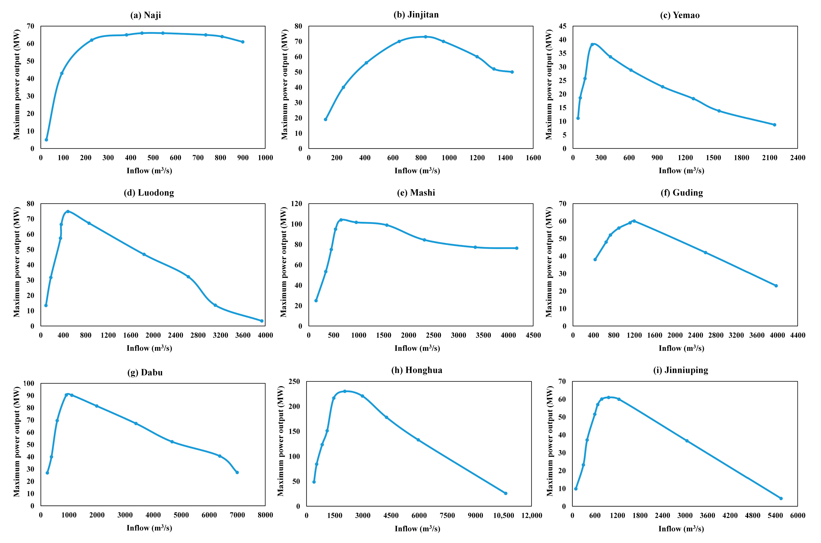
This paper takes the weekly plan of 34 cascaded hydropower stations under the jurisdiction of the Guangxi power grid as an example. Figure 3 shows the relation of the studied hydropower stations. A week in July during the flood season was selected to study, and the maximum power generation model was used to make the weekly plan. Most of the cascaded hydropower stations in Yujiang River, Liujiang River, and Guijiang River on the Guangxi power grid are low-head hydropower stations. After calculation and analysis, we found that apart from Naji, Jinjitan, Yemao, Luodong, Mashi, Guding, Dabu, Honghua, and Jinniuping Hydropower Stations, the differences in power output are relatively insignificant for the other hydropower stations regardless of considering the fitted curve or not. Excluding these nine hydropower stations, the remaining ones have a total power generation ranging from 56,400 MWh to 62,448 MWh over the course of these seven days. Therefore, in order to study the impact of fitted curves on power output, a total of 9 low-head hydropower stations including Naji, Jinjitan, Yemao, Luodong, Mashi, Guding, Dabu, Honghua, and Jinniuping were selected for analysis.

The daily inflow–maximum power output curve is obtained by fitting the historical data according to the method in Section 2, so it is also called the fitted curve. According to the inflow–maximum power out curve demonstrated in Figure 4, which perfectly reflects the serious impact of hindered power output, it can be easily seen that they have the same variation trend. With the increase in inflow, their maximum power output increases first and then decreases. What is more, when a hydropower station’s inflow is more than others, its decline is even greater. Considering this factor, the final results are shown in Figure 5, Figure 6 and Figure 7:

Figure 5 shows the comparison of the weekly plan of the above nine power stations considering the fitted curve, the weekly plan without considering the fitted curve, and the actual results. Considering the fitted curve is to consider the daily inflow–maximum power output curve, then use the expected power output curve and the daily inflow–maximum power output curve to limit the power output according to the method in Section 2. Since the selected time period for the case study falls within the flood season, the fitted curve plays a major role compared to the expected power output curve. Not considering the fitted curve means directly using the expected power output curve as the constraint of the power output. Therefore, according to Figure 5, through comparative analysis of the power output process of hydropower stations in various river basins, it can be concluded that whether or not the fitted curve is considered in the optimal scheduling, there are different degrees of error between the planned and actual results. The main reason for the error is that the weekly plan is usually made this Thursday for the next week, so the actual inflow and the network loads may have a huge error from the prediction. This leads to a continuous adjustment of power output decisions in the actual process for the scheduling plan may greatly differ from the previous plan. However, the errors between considering the fitted curve and not considering the fitted curve are different. It can be easily seen that on most days, the power output when considering the fitted curve is 2–8 MW less than that when not considering the fitted curve, which is closer to the real power output and has less error. So, when considering the fitted curve and the expected power output curve simultaneously, the scheduling plan we derived is more similar to the real ones and more feasible than the results under the circumstance that only the expected power output curve is considered. Especially for Dabu and Jinniuping hydropower stations, the maximum value of error is 5 MW and 4 MW, respectively, when considering the fitted curve while that reaches up to 11 MW and 8 MW without considering the fitted curve. Meanwhile, the larger the power output, the greater the error. The actual power output of Honghua hydropower station on the first day is 8 MW less than that considering the fitted curve, and 16 MW less than that not considering the fitted curve. The cause of these phenomena is the uneven inflow, leading to power output hindered. In some periods of these stations, the expected power output curve is used to calculate power output, so in flood season they can work with the maximum power output. In fact, there is power output hindered when calculating the daily average flow because inflow in a day is uneven, so the power output of some stations like Naji and Dabu cannot reach the maximum value all the time.

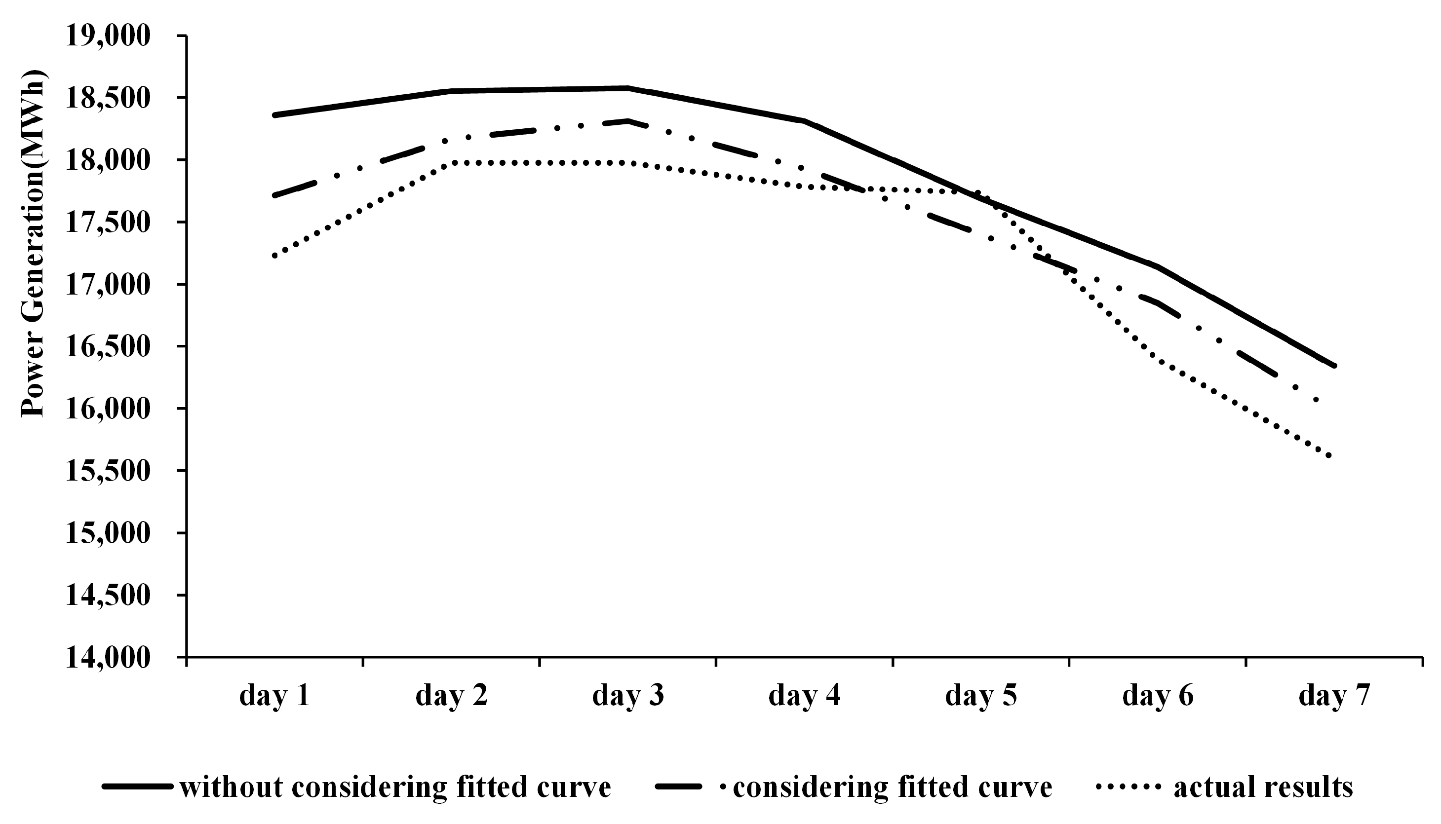
Figure 6 and Figure 7 also effectively illustrate the same phenomenon since the total power generation is derived from the power output, so the results are similar to what Figure 5 reflects. Figure 6 shows the comparison of daily total power generation in three conditions of all nine hydropower stations. It can be seen that the average error when considering the fitted curve is 236.57 MW, while that is 610.29 MW when not considering the fitted curve. What is more, when we kick off the relation between inflow and maximum power output, the power generation in six of seven days is more, reflecting the impact of hindered power output and proving that this model is practical. Figure 7 shows the comparison between the total power generation in three conditions of each station. By comparing, it can be observed that the total power generation of the nine hydropower stations when considering the fitted curve is smaller than that when not considering the fitted curve. Except for the Honghua hydropower station, the total power generation of the other eight hydropower stations is much closer to the actual situation when considering the fitted curve. A possible reason for this may be that on the fifth day, the inflow of Honghua hydropower station is even enough that the fitted curve on that day is unsuitable. Therefore, considering the limitations of the fitted curve on power output may result in the theoretically total power generation being smaller than the actual results. These reasons may have caused the planned power output of the Honghua hydropower station to be smaller than the actual power output on that day, resulting in a smaller total power generation than the real situation. In conclusion, the proposed model in this paper can decrease the impact of hindered power output, making the weekly plan more similar to real conditions.

4. Conclusions

In this paper, a mid-term optimization scheduling model is proposed for low-head cascaded hydropower stations considering the unevenness of water inflow and the hindered power output. This model controls power output by using the expected power output curve and the daily inflow–maximum power output curve together. Nine hydropower stations on the Guangxi power grid are studied, and the results whether the fitted curve is considered or not are compared with the actual results. The results show that (1) considering the fitted curve, the scheduling plan is more in line with the actual conditions, resulting in an error reduction of 2–8 MW compared to that when not considering the fitted curve. (2) When considering the fitted curve, the total daily power output of the nine studied stations has a smaller error of 61% compared to that when not considering it, and the total power output for each station over seven days is also smaller.

It can be observed that the unevenness of inflow has a significant impact on the optimal scheduling of hydropower stations, especially for stations with small installed capacities. In addition, the hindered power output further reduces the accuracy of calculations and complicates the optimal scheduling problem. Therefore, the model proposed in this paper partially addresses this problem and improves the accuracy of power output calculation for low-head hydropower stations with uneven inflow.