Prediction of Carbon Price in EU-ETS Using a Geometric Brownian Motion Model and Its Application to Analyze the Economic Competitiveness of Carbon Capture and Storage

Abstract

To achieve carbon neutrality, many countries and regions are making efforts to promote the commercialization of greenhouse gas (GHG) mitigation technologies using emissions trading systems (ETSs). Accurate predictions of when the cost of GHG reduction technologies will become competitive below carbon prices could be invaluable to engineers and policy makers. In this study, carbon price movement in the EU-ETS was analyzed using a geometric Brownian motion (GBM) model. Using daily price data for the last 10 years, it tested whether the price pattern of the latter three years could be predicted by applying the first seven years of data to the GBM model. The results showed that the GBM model could well predict the upper and lower bounds of the actual carbon price. Based on the acceptable predictability of the GBM model, simulations were performed using carbon price data over the last decade, showing that carbon prices would reach around 200 EUR/tCO₂ by the start of 2026. This is higher than the cost of CO₂ avoided evaluated from the costs of commercial-scale carbon capture facilities for coal-fired power plants. This means that carbon capture technologies in the coal-fired power sector could become economically competitive within the next several years.

1. Introduction

Since the Paris Agreement was adopted at the 21st Conference of the Parties (COP) on Climate Change, countries accounting for more than 95% of global GHG emissions have submitted intended nationally determined contributions (INDCs). Accordingly, the climate change response system has operated with the participation of most countries around the world. In June 2015, for example, the Republic of Korea submitted an INDC with the goal of reducing emissions by 37% compared to business as usual by 2030 to comply with the Paris Agreement. In order to more actively contribute to achieving a carbon net zero target by 2050, Korea additionally announced at COP26 an improved proposal to reduce emissions by 40% compared to 2018 (727.6 Mt CO₂) by 2030 [1]. This target was submitted to the UN in December 2021 as Korea’s new INDC. This corresponds to an average annual reduction rate of GHG emissions of 4.17%, which is a very challenging target compared to that of other major countries (EU 1.98%, UK 2.91%, US 3.07%, Canada 2.38%, and Japan 3.56%). In March 2023, while the total emissions target for the INDC was fixed the same as for the 2021 INDC, the emissions target of each sector was fine-tuned.

Table 1. Targets and their baselines of Korea’s INDC.

INDC in 2018 (MtCO2-eq)		Updated INDC in 2021 and 2023 (MtCO2-eq)
(Base) 2030 BAU	INDC Target (Reduction Rate)	(Base) Total National GHG Emissions in 2018	INDC Target (Reduction Rate)
850.8	536.0 (37%)	727.6	436.6 (40%)

shows the baseline emissions and targets of Korea’s INDC proposals in 2018 and after 2021.

Table 2. Sectoral emissions targets of Korea’s INDC for 2021 and 2023 and major reduction measures.

Sector	Base Emissions in Year 2018	INDC Targets in Oct 2021	INDC Targets in Mar 2023	Major Reduction Measures
(Unit: MtCO2-eq)	727.6	436.6	436.6
Power generation	269.6	149.9	145.9	Renewable energy, reduction in coal-fired power
Industry	260.5	222.6	230.7	Process improvements, conversion of fuel and raw materials
Building	52.1	35.0	35.0	Zero-energy building, smart energy management
Transportation	98.1	61.0	61.0	Expansion of eco-friendly vehicles, increase in biodiesel mixing ratio
Agriculture, livestock farming and fisheries	24.7	18.0	18.0	Expansion of low-methane feed, reduction in fertilizer use
Waste management	11.0	9.1	9.1	Waste reduction and recycling, expansion of bioplastics
Hydrogen	-	7.6	8.4	Water electrolysis hydrogen technology, byproduct hydrogen
Etc.	5.2	3.9	3.9
Carbon sinks		−26.7	−26.7	Sustainable forestry, urban green space
CCUS		−10.3	−11.2
Overseas reduction		−33.5	−37.5	Forestry, renewable energy business

summarizes the sectoral emissions targets of the INDC for 2021 and 2023 [2].

According to the INDC proposals of each country, efforts to develop carbon dioxide mitigation technologies are becoming more important. In Korea, for example, a plan was established to achieve its INDC goal via energy-mix improvements in the power generation sector; the active adoption of new facility technologies and raw material conversion in the industrial sector; the development of building energy savings and management technologies; the expansion of electric vehicles in the transportation sector; low-carbon agricultural and livestock technologies; waste recycling; the expansion of hydrogen supply; the creation of GHG sinks using forests and oceans; overseas emissions reduction through clean development mechanism projects; and the development of carbon capture, utilization and storage (CCUS) technologies. Table 2 shows representative GHG reduction measures to achieve emissions targets in each sector [2]. A policy tool capable of accelerating the pace of development in all these technology areas is an emissions trading system (ETS).

An ETS is generally a cap-and-trade scheme in which regulators assign an acceptable amount of GHGs that a company can emit from its system, and then the company trades the shortfall or surplus of emissions allowance. It aims to internalize negative externalities generated in the production process into management by allowing private companies to purchase emissions allowances corresponding to the amount of GHGs they emit into the atmosphere [3]. The world’s first ETS is the EU-ETS, opened in 2005, accounting for about 90% of the global transaction volume as of 2021 [4]. In 2021, the EU raised its target for the reduction rate of the total emissions allowance to mitigate GHGs by at least 55% by 2030 compared to 1990 levels. In addition, the EU is implementing a climate policy to completely abolish the free allocation of emission allowances by 2032 with the goal of reaching carbon neutrality by 2050. These policy measures have recently been acting as a factor driving the rise in the price of emission allowances in the EU-ETS. Since the price of emission allowances can affect the timing of the introduction of new technologies, the regulatory authorities operating the emissions market are implementing a market stabilization system to prevent sudden fluctuations.

Companies with high GHG emissions are faced with the choice of accepting the cost of purchasing credits from the market with existing production methods or adopting new low-carbon production technologies. In both options, companies need a criterion to compare the cost per ton of CO₂ avoided calculated from the installation and operation of new technology and the expected price of CO₂ allowances from a long-term perspective. Prediction of the carbon price needs an appropriate modeling method for price movements. In the literature, the modeling of carbon prices is still open with various methodologies being tried, such as the variance gamma model [3], geometric Brownian motion (GBM) model [5], generalized autoregressive conditional heteroscedasticity models [6], convolution neural network model [7], and artificial intelligence methods [8]. One of the common approaches is to assume that price of emission allowances follows a geometric Brownian motion or its variant models [9,10,11,12,13,14]. Carbon prices are mainly affected by the level of strength of climate policies and the costs that companies have to pay [3]. Individual countries and regions operating the ETS are introducing market stabilization systems such as the minimum price system to prevent corporate decision-making power for GHG reduction investment from weakening [3]. These systems, combined with recent changes in the global political and energy environment, are acting as one of the causes of the rise in carbon prices. In general, energy commodity prices show mean-reversion characteristics [12]. Carbon credits have similar characteristics to energy commodities, but log-return data deviate from a normal distribution because the supply of carbon credits is also influenced by non-market factors such as politics and social consensus on environmental issues. Despite these data characteristics, GBM models have been widely used to predict the price of ETS carbon credits [5,12,13,14], for example, in the study on the effect of floor price [13].

The effect of the carbon credit price on the introduction of various new technologies for GHG mitigation has been studied by several researchers over the past decade. Flora and Vargiolu [3] studied the effect of a minimum carbon price system in an economic analysis of the process of converting oil-fired power generation to photovoltaic power generation. Compernolle et al. [14] analyzed the economic feasibility of CO₂ enhanced oil recovery technology according to the price of carbon credits. Lukas and Welling [5] reported the impact of CO₂ prices on the timing of climate-friendly investments by several companies sharing a supply chain. Manaf et al. [15] developed a platform to analyze investments in low-carbon emissions technologies based on CO₂ price predictions.

CCUS technology is considered as one of the representative GHG mitigation technologies. In the carbon-neutral scenario proposed by the IEA, the contribution of CCUS technology is 15% of the total GHG reduction [16]. In order to implement CCUS technologies, the commercialization of carbon capture technology is required first. There are a few carbon capture facilities in operation where cost analysis is available [17].

The purpose of this study is to predict the future carbon price of EU-ETS. The results were applied to analyze the economic feasibility of carbon capture and storage (CCS) technology, that is, to develop a basic but practical methodology to determine when to invest in CCS commercialization. The GBM model explained in Section 2 was applied to historical price data of the EU-ETS, which has the most reliable data with the largest market size and a long trading history. In Section 3, the prediction ability of the GBM is verified. In Section 4, the future carbon price is predicted using EU-ETS data over the last decade and then compared with the cost of the CCS to predict when the two prices will balance out. Section 5 summarizes the conclusions of this study.

2. Geometric Brownian Motion Model

One of the common ways to estimate variables under uncertainty is a Monte Carlo simulation, which is a computational technique to utilize randomly repeated numerical experiments. There are many sub-models of a Monte Carlo simulation for option price [9,18]. In this study, the geometric Brownian motion (GBM) model was used for a random trial method to produce a statistical distribution of EU allowance (EUA) future price. The GBM is technically a Markov process following a random walk, which has been widely applied not only in finance but also in science and engineering. When applied to EUA price analysis, it means that information from historical price data is already integrated, and the future prices are conditionally independent of past prices. The logarithmic value of the change in carbon price over any period is normally distributed, with a distribution depending only on the length of the period.

The GBM equation for the price of CO₂ allowance is as below [9],

$$\frac{dP}{P}=\left(\mu \Delta t+\sigma ϵ\sqrt{\Delta t}\right)$$

(1)

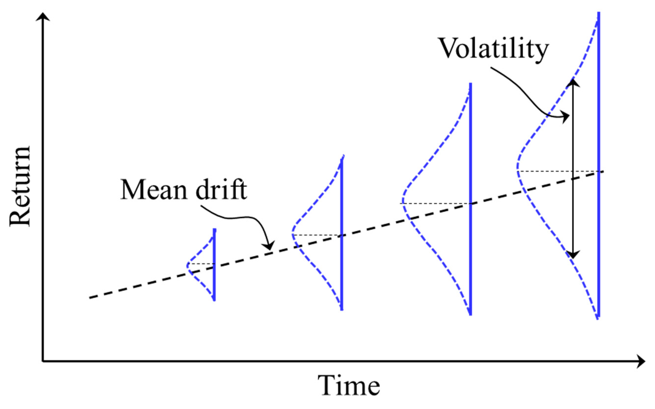
where P, dP, μ, σ and ϵ are the price of CO₂ allowance, the price change of CO₂ allowance, the expected return during Δt, the standard deviation of returns during Δt, and the random number, respectively. The first part of the right-hand side indicates the average trend (mean drift) in price movement, and the second one represents the random walking (volatility) of price. Equation (1) describes the price of CO₂ allowance, which follows a series of time steps, where the expected price is the sum of mean drift ($\mu \Delta t$) and a random volatility ($\sigma ϵ\sqrt{\Delta t}$), as shown in Figure 1.

The application procedure of Equation (1) to predict the future price of CO₂ allowance using historical daily price data is summarized in

Table 3. Procedure of GBM analysis using daily price of CO₂ allowance.

Step	Data Process
(Step 1)	Calculate daily changes using the historical daily price data of CO2 allowance [19]
(Step 2)	Calculate daily drift (average of daily change) and daily volatility (standard deviation of daily change)
(Step 3)	Simulate price of CO2 allowance for a given period using Equation (1)
(Step 4)	Repeat (Step 3) N times (N = 10,000 was used in this study, as explained in Section 3)
(Step 5)	Summarize statistics

. The analysis methodology in Table 3 was implemented in Excel of Microsoft 365.

3. Predictive Potential of the GBM Model

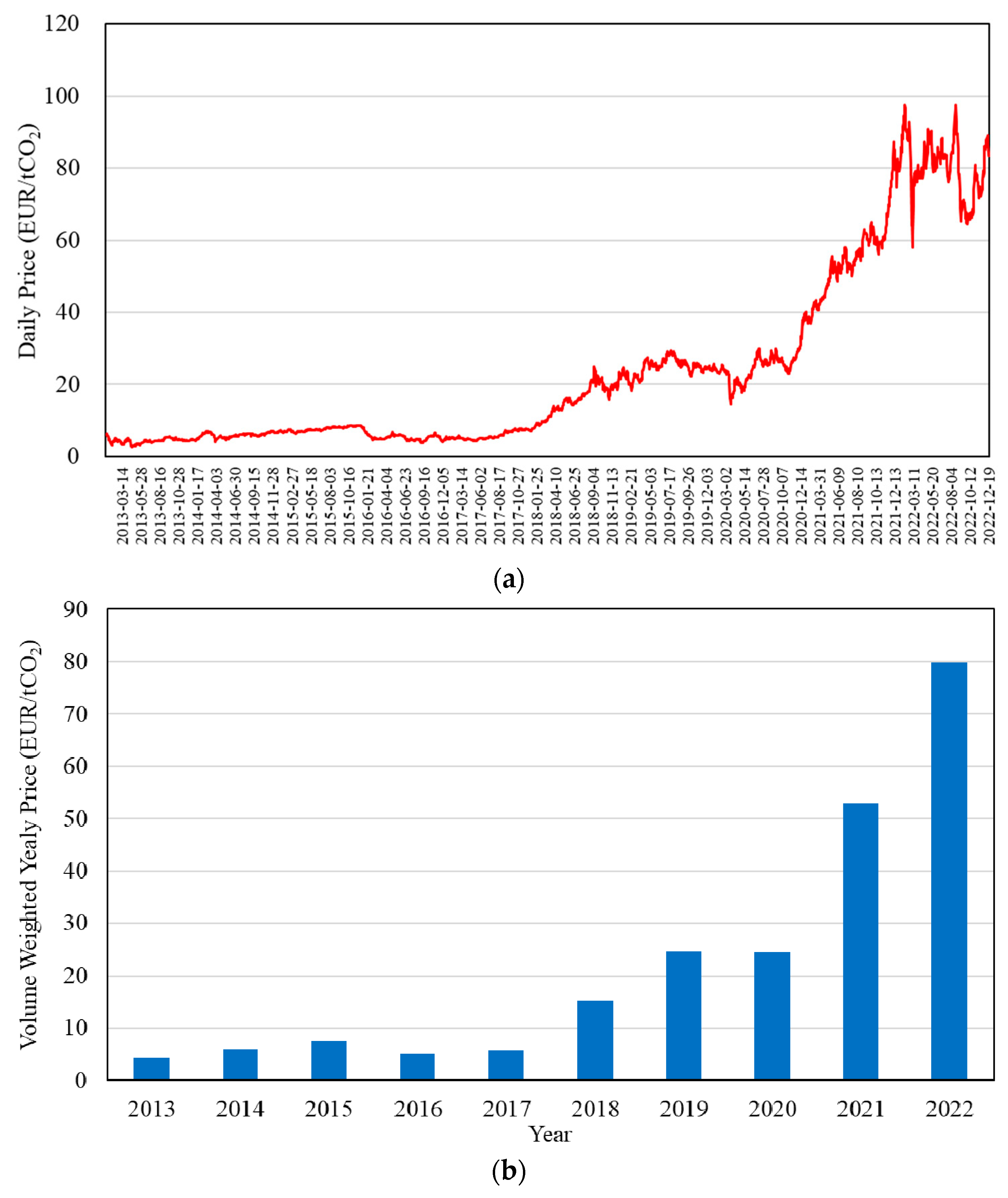
Figure 2a shows the 10-year graph of EUA prices from 2013, when the 3rd phase of the EU-ETS began, to 2022 [19]. The volume-weighted average annual price shows a steady upward increasing pattern, as shown in Figure 2b. Since 2019, when the market stability reserve was introduced, the price has been steadily rising. In 2020, the European Commission proposed more challenging climate change targets for 2030. From 2021, when the 4th phase of the EU-ETS began, the free allocation of allowance is further reduced, and the total supply of EUA is reduced at a rate of 2.2% annually. As a result, the price of EUA is rising more steeply.

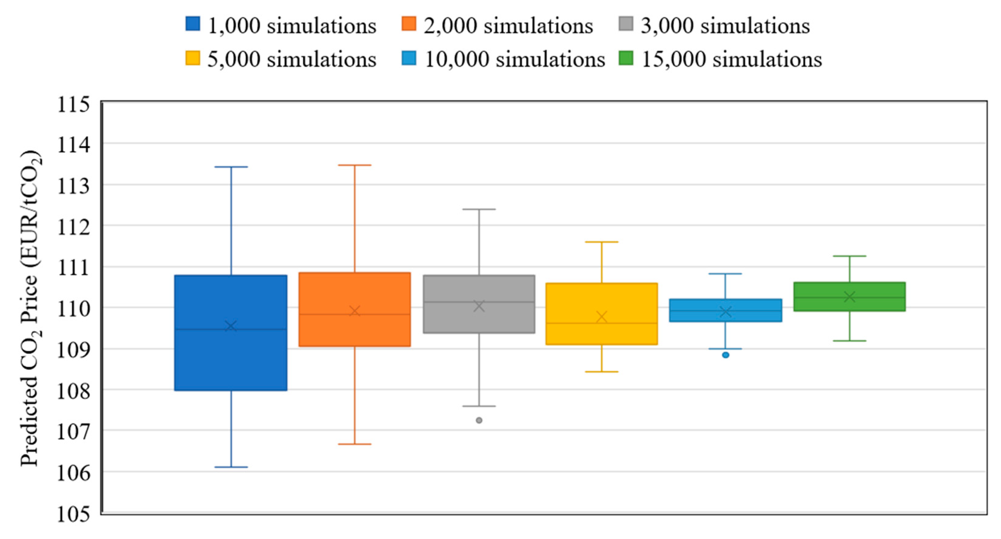
The effects of the number (N) of simulations and the length (ω) of historical data used for GBM were analyzed to determine the appropriate simulation conditions required for GBM analysis. For the test of GBM simulation, the EU-ETS data for 10 years (2013–2022) were applied to Equation (1), the simulation was repeated N times, and the average price after 1 year was evaluated from the N simulation realizations. As for the number of simulations (N), the change in average value was analyzed while applying six conditions from N = 1000 to 15,000. Figure 3 shows a box plot of the predicted average values obtained by repeating 30 sets for the specific number (N) of GBM simulations. As the number (N) of numerical experiments increases, the range of the average value distribution becomes narrower with a smaller variance. However, the variance of the average does not change significantly under the condition of N = 10,000 or more. Therefore, in this study, N = 10,000 was selected as the number of GBM simulations.

To analyze the effect of the modeling period length (ω) used in GBM simulation, EU-ETS data from the last decade were divided into the latter three years (2020–2022) and the first part of the varying modeling period. A numerical experiment was conducted to predict the price of the latter three years by applying the price data of the varying modeling period (ω = 3 to 7 years) to the GBM model.

Table 4. Definition of modeling and validation periods for GBM tests.

Test No.	Validation Period	Modeling Period (ω)	$\mathbf{Average} \mathbf{Daily} \mathbf{Change} \left(\mathit{\mu }\right)$	$\mathbf{Standard} \mathbf{Deviation} \mathbf{of} \mathbf{Daily} \mathbf{Change} \left(\mathit{\sigma }\right)$
Test 1	667 market days (3 years, 2020–2022)	7 years (2013–2019)	0.000917	0.03875
Test 2		6 years (2014–2019)	0.001332	0.03241
Test 3		5 years (2015–2019)	0.001211	0.03173
Test 4		4 years (2016–2019)	0.001323	0.03376
Test 5		3 years (2017–2019)	0.002635	0.03180

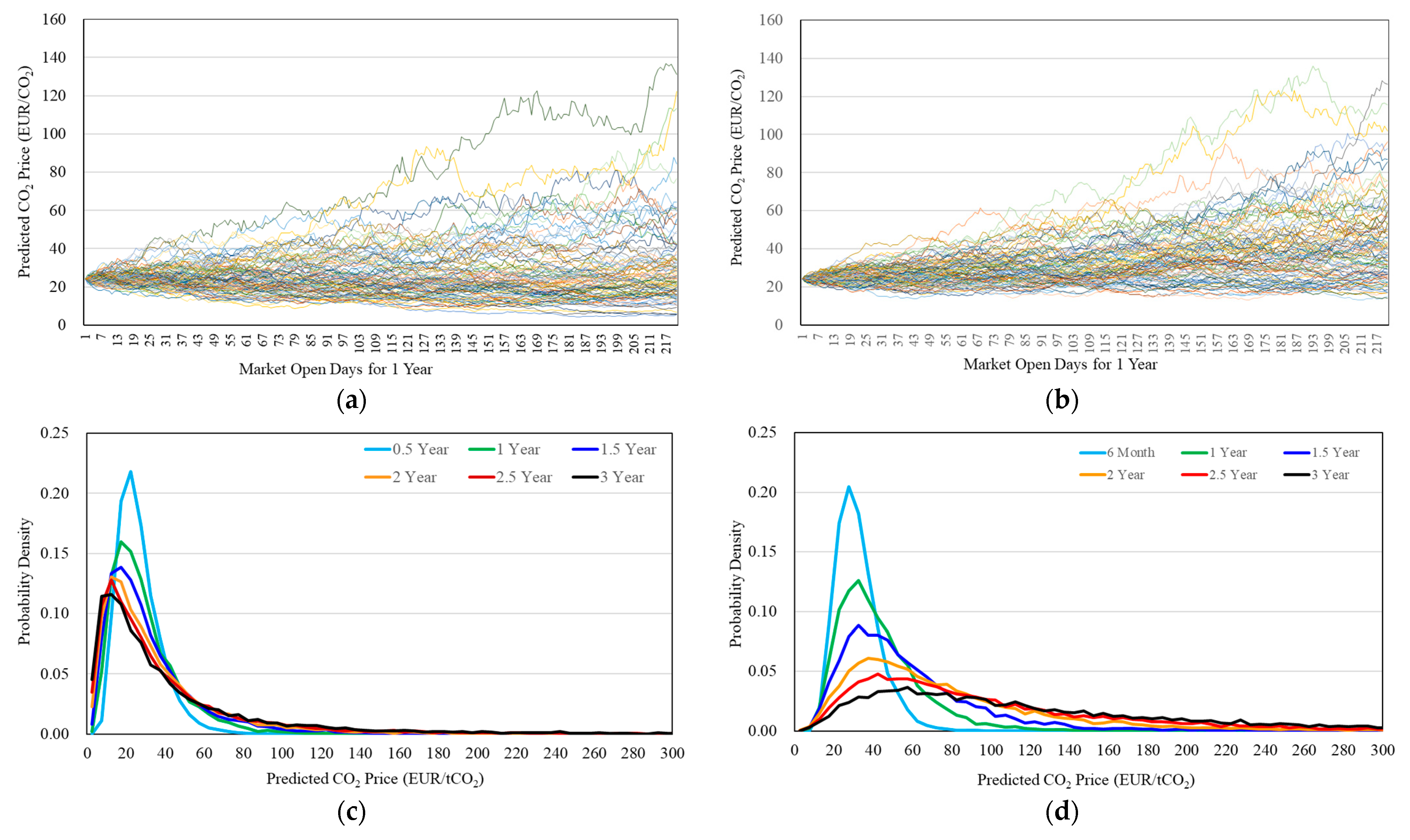
shows test conditions for the five lengths (ω) of modeling period used in the GBM simulation. According to the results obtained in Figure 3, simulations were performed 10,000 times under each test condition. Figure 4a,b show 100 realizations, which are part of the 10,000 simulations of Test 1 and Test 5. Because the mean drift ($\mu$) and volatility ($\sigma$) change with the length (ω) of modeling period used for price prediction, the simulations of Test 1 and Test 5 show quite different results. Since the magnitude of price change after 2017 rises significantly compared to the previous period before 2017, as shown in Figure 2a, the average daily drift of Test 5 is about 2.8 times that of Test 1, as summarized in Table 4. As a result, the simulation result of Test 5 (Figure 4b) predicts a stronger price rise than the predicted scenario of Test 1 (Figure 4a). Figure 4c,d are the probability density distributions of carbon prices obtained from the results of Test 1 and Test 5 every 6 months. As time elapses, the probability density of the price is more widely distributed due to the spread of the volatility component.

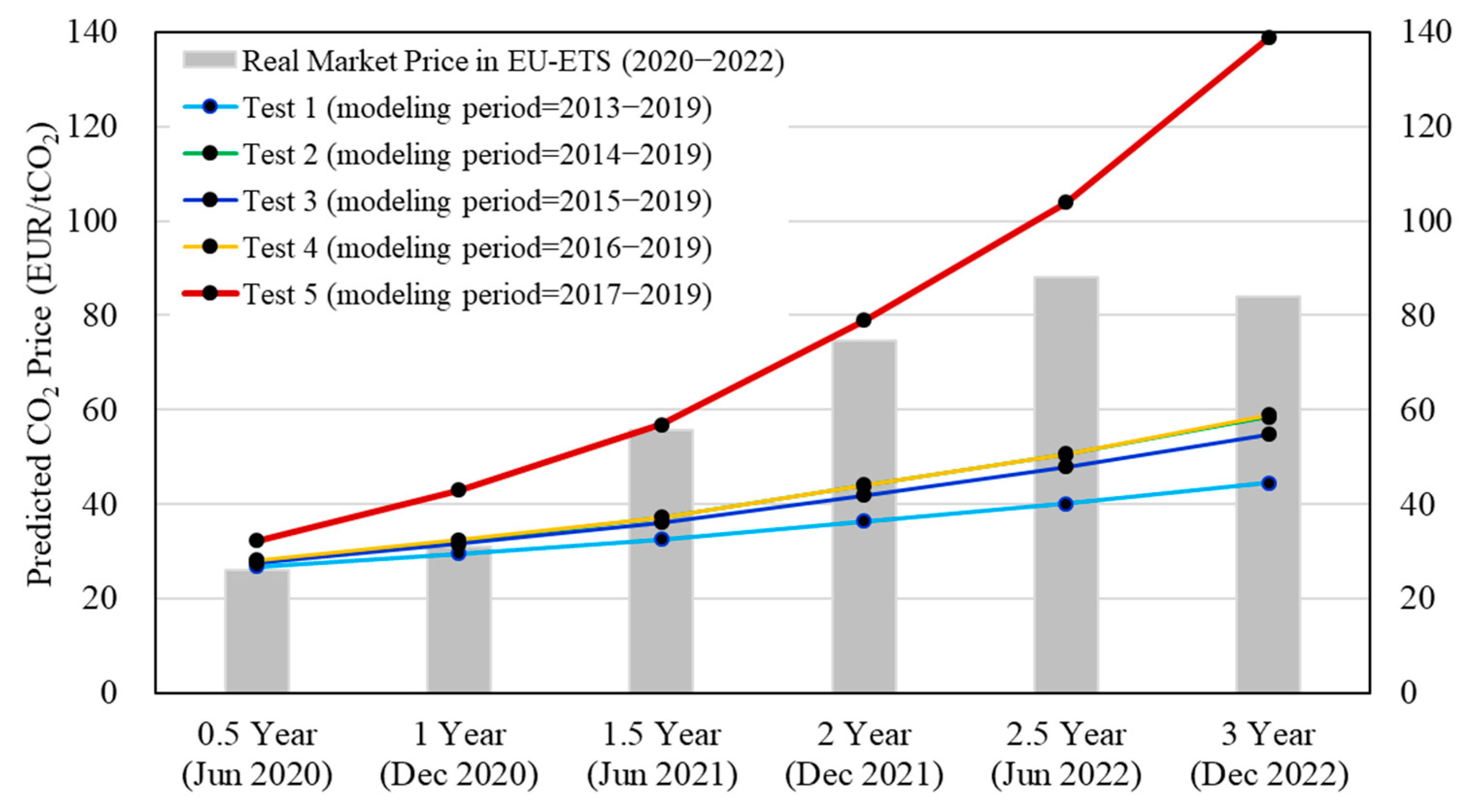
Figure 5 compares predicted carbon prices averaged at regular intervals (every six months) from 10,000 numerical experiments under each test condition with EU-ETS real-price data over the last three years (2020–2022). Due to the length (ω) of modeling period used in each GBM simulation, the average drift and volatility values are different, as shown in Table 4, resulting in different predicted price patterns for the three-year (2020–2022) validation period. According to Figure 5, price patterns can be categorized into three groups: Test 1, Tests 2–4, and Test 5. As summarized in Table 4, while the standard deviation of daily change does not show a large difference with respect to the length of the modeling period in the tests, the price pattern group is determined by the large difference in the magnitude of average daily change. The simulation results of Tests 1 to 4 predicted the actual EUA price at the time of the first 6 months and 1 year with an error range of 5 to 10% or less. On the other hand, for the actual EUA price after 1.5 years and 2 years, the results of Test 5 predicted well within the error range of 5% or less.

Forecasting the price of EU-ETS is a complex task that requires considering various factors such as economic conditions, energy demand, government policies, and geopolitics. The recent Russian–Ukrainian war is a typical example of how geopolitical factors affect carbon prices. The war has forced some investors facing margin calls on their energy investments due to soaring natural gas prices and Russian investors at risk of an asset freeze under Russian sanctions to pull their funds out of the EU-ETS market [20]. This caused EU-ETS carbon prices to drop by about 20% in the short term following the Russian–Ukrainian war. On the other hand, for geopolitical reasons since the war began, the EU is accelerating energy efficiency improvements and renewable energy supplies in order to reduce its high energy-dependence on Russia [21]. If these EU efforts are successful, the long-term impact of the Russian–Ukrainian war on the EU-ETS will be reduced, and carbon prices will normalize.

Historical price data can provide useful information and insights, but they cannot be the sole basis for predicting future prices. EUA price movements are inherently uncertain and subject to many unpredictable events and socio-political changes, such as the example described in the above paragraph. Nevertheless, in Figure 6, the movement of the actual EUA price for the three years from 2020 to 2022 changes between the five (Test 1 to 5) price scenarios using the previous price data in a large frame. Therefore, the results of various price prediction scenarios determined by adjusting the modeling length (ω) of historical price data applied in GBM can be used as a means of obtaining information on the upper and lower limits of future prices of emission allowances.

4. Cost Competitiveness of CCS Compared to Estimated EUA Price

In the previous section, the potential of the GBM model to predict the range of future prices of EUAs was described. In this section, the GBM model is applied to analyze when the cost of carbon capture application becomes capable of competing with EUA prices. In order to achieve carbon neutrality, it is necessary to effectively absorb and treat CO₂ emitted from power plants, steel and iron processes, cement factories, etc.; therefore, the importance of CCUS technology is emerging. In order to achieve the net zero goal of global CO₂ emissions by 2070, the cumulative reduction contribution of CCUS in the energy sector has to reach 15% according to the IEA’s sustainable development scenario [16]. CCUS basically requires the development and maturation of carbon capture technologies. It is difficult to determine the economic feasibility of carbon capture with a single criterion because the cost of carbon capture varies over a wide range depending on the concentration (partial pressure) of CO₂ in the flue gas for each industry group. For example, in natural gas processing plants with a high CO₂ concentration up to 5000 kPa [17], the carbon capture cost is 15 to 25 USD/tCO₂ [22]. In the case of coal-fired power plants with low CO₂ partial pressure (12.2 to 14.2 kPa) [17], it is reported to be 50 to 100 USD/tCO₂ [22]. There are many different types of CCUS. Carbon capture and utilization (CCU) technologies are known to be at an earlier stage of implementation than carbon capture and storage (CCS) technologies [23]. On the other hand, according to the IEA, as of 2070, the carbon capture volume of the power generation sector is expected to account for the largest proportion of the total carbon capture volume, up to 40% [16]. Therefore, in this study, the coal-fired power generation sector was selected for the analysis of the time to secure the economic feasibility of CCS costs.

Even limited to the coal-fired power generation sector, the range of carbon capture costs is quite wide in the literature [17,22]. This is because the cost of carbon capture is affected by various factors such as the technological level of each country, electricity market conditions including power generation cost, power plant construction cost, and labor cost [24]. In the power generation field, CCS facilities that are currently operating at a commercial level are rare, and most of them are operated on a pilot or demonstration scale [25]. Therefore, most studies on the cost of CO₂ capture have been conducted in pilot-scale power plants [24,26], and there have not been many cases in large-scale power plants close to commercialization. Figure 7 shows data widely cited in recent research on the cost of carbon capture in the coal-fired power generation sector [17]. According to the trend (blue dotted line) in data denoted by points in Figure 7, where the average exchange rate between the US dollar and the Euro over a 10-year period (2013–2022) is applied [27], the cost of carbon capture in the power sector is expected to decrease to around 40 EUR/tCO₂ within the next several years. However, it is important to understand that some cost studies of carbon capture in commercial-scale power plants contain optimistic expectations for future carbon capture technologies.

Of the total cost of a CCS chain, the cost of carbon capture accounts for the largest share. The cost of transport and storage of captured carbon varies greatly from case to case depending on the flow rate of carbon, the transportation distance from the capture plant to the storage site, and the storage conditions [17]. It is generally known that carbon capture accounts for about 75% of the total CCS cost [28]. Taking this into account, predicting the future cost of CCS from the cost trend of carbon capture is shown by the solid blue line in Figure 7, where CCS costs are expected to fall below 50 EUR/tCO₂ after 2026.

On the other hand, there are uncertainties that could exacerbate the optimistic projections of the cost trend line of carbon capture and CCS in Figure 7. Some of the data in Figure 7 used to determine the trend line of carbon capture have been criticized for not sufficiently disclosing the underlying data of cost estimation [29]. In addition, the data group creating cost downtrends rely on design expectations for not-yet-operating, to-be-commissioned plants [17]. Moreover, changes in the global economic environment, such as the recent surges in interest rates and raw material prices, could lead to higher plant construction costs, which could also distort the cost forecasts of carbon capture distributed in the lower right corner in Figure 7. In the case of South Korea, assuming that the construction and operation period of a coal-fired power plant are 4 years and 30 years, respectively, it is estimated that the construction cost of a power plant will account for about 34% of the net cash flow generated during the operation period [30]. If the proportion of costs during the construction period increases, it could worsen the cash flow of the plant and increase the abatement costs of a carbon capture facility. Therefore, contrary to the prediction of the trend line in Figure 7, there may not be a significant change in costs in the near future despite advances in carbon capture technology.

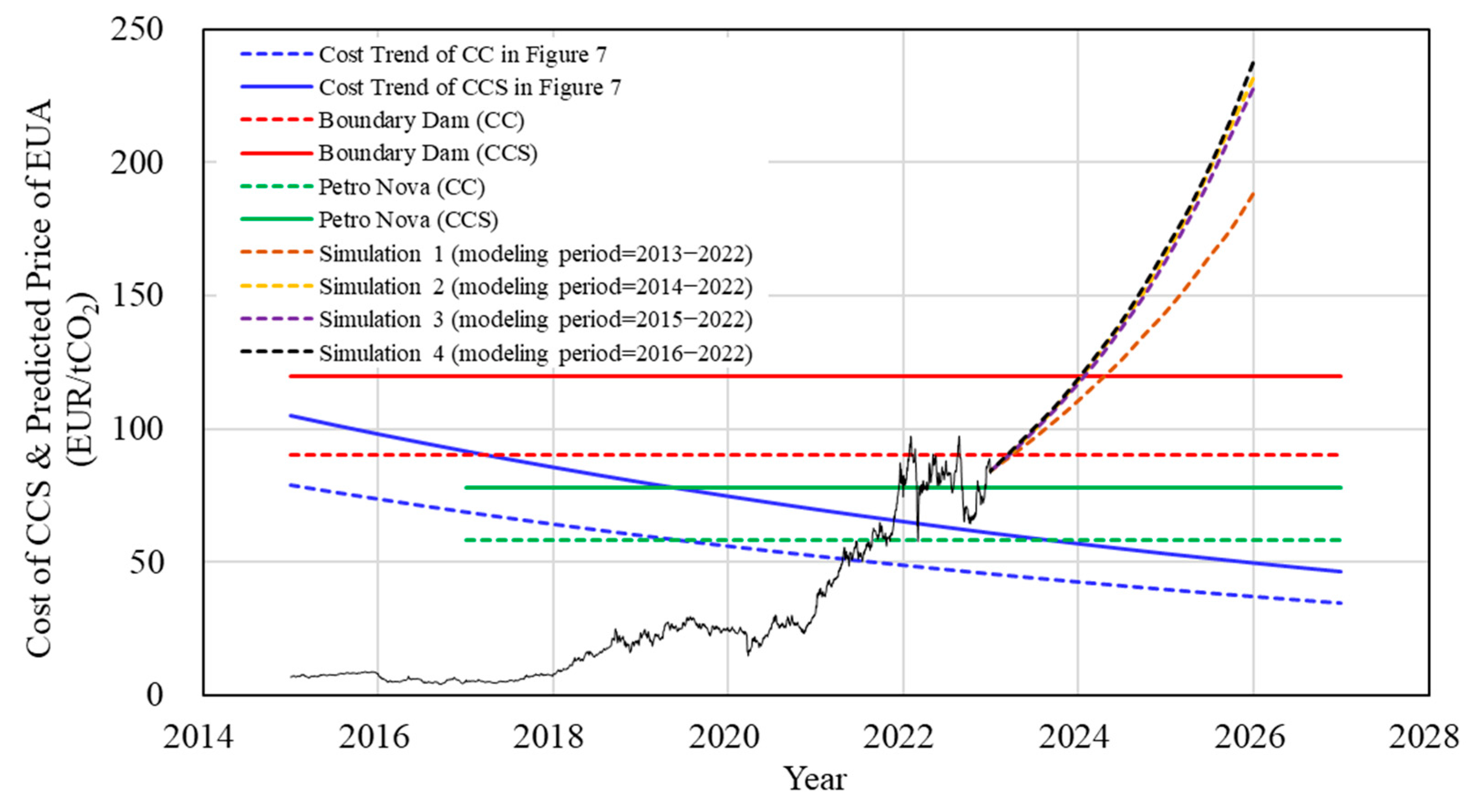
Given these uncertainties not included in the cost trend projections of carbon capture shown in Figure 7, it is assumed that the estimated CCS costs of the representative power plants operated at near-commercial scale such as Boundary Dam and Petra Nova could remain constant over the next few years, as shown in Figure 8. Under these pessimistic assumptions, the CCS cost of Petra Nova (approximately 80 EUR/tCO₂, solid green line) is roughly equivalent to the level of current EUA prices, and that of Boundary Dam (approximately 123 EUR/tCO₂, solid red line) is expected to be economically feasible within the next 2~3 years. Figure 8 also shows the results of forecasting CO₂ prices over the next 3 years (2023–2025) while adjusting the length of the modeling period from EU-ETS daily price data for the past 10 years (2013–2022).

Table 5. Simulation conditions and their statistical results for predicting the three-year (2023–2025) price of EU-ETS using the GBM model.

Simulation No.	Prediction Period	Modeling Period (ω)	$\mathbf{Average} \mathbf{Daily} \mathbf{Change} \left(\mathit{\mu }\right)$	$\mathbf{Standard} \mathbf{Deviation} \mathbf{of} \mathbf{Daily} \mathbf{Change} \left(\mathit{\sigma }\right)$
Simulation 1	667 market days (3 years, 2023–2025)	10 years (2013–2022)	0.001218	0.03702
Simulation 2		9 years (2014–2022)	0.001520	0.03260
Simulation 3		8 years (2015–2022)	0.001468	0.03200
Simulation 4		7 years (2016–2022)	0.001566	0.03340

lists the conditions and the results of the GBM simulation for CO₂ prices in Figure 8, where carbon prices are expected to reach levels of around 200 EUR/tCO₂ by the start of 2026. Similar to the results of five tests in Section 3, there is no significant difference in the standard deviation of daily price change in the simulations. On the other hand, the average value of daily price change is divided into two groups (Simulation 1 and Simulations 2–4), and the predicted CO₂ price pattern is divided into the corresponding two groups as shown in Figure 8. The meaning that can be drawn from Figure 8 is that, even considering various uncertainties, the cost of CCS technology implemented in coal-fired power plants may become cost-competitive compared to the purchase price of EUA within the next several years. Therefore, it is necessary to actively promote the introduction of CCS technology in the field of coal-fired power generation at this moment.

5. Conclusions

In order to analyze the cost-competitiveness of carbon capture application technology against carbon prices in the EU-ETS market, a study on carbon prices was performed using a geometric Brownian motion model. First, the EU-ETS carbon price data for the past 10 years (2013–2022) was divided into two periods, and the price data of the previous part was applied to the GBM model to predict the price for the latter three years (2020–2022). The ability of the GBM model to predict the carbon price was validated through the existence of the actual carbon price in emissions markets within the price range of the GBM simulations obtained by varying the length of the modeling period.

The future cost trend of CCS technologies implemented in coal-fired power plants reported in the literature was analyzed. Carbon prices over the next 3 years (2023–2025) were predicted using the GBM model, adjusting the length of modeling period from the EU-ETS daily price data for the past 10 years (2013–2022). According to the GBM simulations, the price of carbon allowance would reach a level of about 200 EUR/tCO₂ within the forecast period. This indicates that CCS technology could become cost-competitive for coal-fired power plants within the next few years. However, there exists uncertainty in both predictions of CCS cost and carbon price because the data used to predict the cost of CCS technology at the commercial scale are insufficient in the literature, and the global economic and political environment is changing rapidly.

The continuous rise in the carbon price through the stable operation of the ETS market has served as a catalyst for the development and commercialization of GHG mitigation technologies. The methodology of this study is not limited to the economic analysis of CCS technology for coal-fired power plants but can be applied to predicting the point of securing cost-competitiveness of GHG reduction technologies in various fields. It can be useful to both engineers and policy makers who need a baseline to determine when to invest in the commercialization of specific GHG mitigation technologies.