Review of Methods for Evaluating the Energy Efficiency of Vehicles with Conventional and Alternative Power Plants

Abstract

The evaluation of the energy efficiency of vehicles in operating conditions is used to solve management and control tasks in intelligent transport systems. The modern world fleet is characterized by an increase in the share of vehicles with alternative power plants (hybrid, electric, and hydrogen fuel cells). At the same time, vehicles with conventional power plants (internal combustion engines) remain in operation. A wide range of modern power plants determines the relevance of studying the advantages and limitations of existing methods of evaluating the vehicle energy efficiency, delineating the application scope and highlighting promising directions for their further development. The article systematizes the methods of evaluation and management of the energy efficiency of vehicles with conventional and alternative power plants. Special attention is paid to the assessment of energy consumption per unit of transport work at the stage of vehicle operation, taking into account various operational factors. The concept of a 3D morphological model of the transport system for evaluating the energy efficiency of vehicles is presented. An algorithm for the optimization of the current transport system configuration according to the criterion of an increase in the energy efficiency indicator is given.

1. Introduction

The implementation of intelligent transport systems contributes to solving such issues as increasing the economy and environmental friendliness of vehicles, ensuring traffic safety, laying rational transport routes, and improving the operation of transport infrastructure. Control objects in such systems are its functional elements: the vehicle or its subsystems and aggregates; traffic flow; and road and transport infrastructure. The improvement of their designs and operating modes can take place according to the criterion of the energy efficiency of vehicles during operation. As a result of the increase in the level of motorization of the population, the development of transport technologies, and the presence of global environmental problems, a wide range of vehicles with different power plants has been formed. Scientists propose several methods based on energy efficiency models of vehicles with conventional and alternative energy systems. The adequacy of these models and the capability of the corresponding methods are only ensured under certain conditions. This determines the relevance of studying the advantages and disadvantages of existing methods, delineating the scope of their application, and highlighting promising directions for further development. The systematization of existing methods according to the category of vehicle, type of power plant, parameters of influence, and limitations of application will help scientists to choose a method taking into account the purpose of their research and technical capabilities. The integration of various energy/fuel consumption models will ensure that relevant transport technologies are taken into account in the algorithms of intelligent transport systems.

In work [1], a generalized classification of methods for evaluating the energy efficiency of wheeled vehicles is given. The advantages and limitations of the methods are defined. The methods of evaluating the energy efficiency of vehicles can generally be classified as follows: (1) universal and only intended for certain vehicle categories and types of power plants; (2) based on the vehicle design features and based on the parameters of the transport system functional elements; and (3) those that do not require direct determination of fuel/energy consumption and those that require specified calculations. In most countries, the main measure of fuel economy is fuel consumption per 100 km and fuel consumption per unit of transport work. In some European countries, the national standard provides the following indicators for comparing the fuel economy of analogs: (1) control fuel consumption, which is determined for all categories of vehicles at specified speed values when moving in a higher gear on a horizontal road; and (2) the fuel characteristic of steady movement. The second indicator characterizes the dependence of the fuel consumption per 100 km of traveled distance on the speed of steady movement in a higher gear on a horizontal road for all vehicle categories [2].

The methods of estimating fuel/energy consumption, in turn, can be conditionally divided into several groups. The methods in the first group are based on measuring the fuel efficiency of vehicles for given driving cycles. The Federal Test Procedure (FTP), the New European Driving Cycle (NEDC), the World Harmonized Light-Duty Vehicles Test Procedure (WLTP), the Highway Fuel Economy Test (HWFET or HFET) cycle, the Extra Urban Driving Cycle (EUDC), and the Urban Dynamometer Driving Schedule (UDDS) test are used to test fuel economy [3]. In [3], the main characteristics of the specified standard driving cycles and the corresponding profiles of speed dynamics are given. However, such testing cannot adequately reflect the real operating conditions in a given region. In [4], the need for local driving cycles is substantiated. Therefore, the authors of [4] proposed a method of determining the local driving cycle (DC) for the further assessment of fuel consumption and harmful emissions of the investigated vehicle. According to this method, the driving cycle for a vehicle of a given technology is characterized by a vector of driving model parameters in a given region. From the statistical sample of such vectors, the one that minimizes the deviation of the vehicle’s fuel consumption from its average sample value is selected. The driving model takes into account the average and maximum values of speed and acceleration of the vehicle, the percentage ratio of its movement modes, the positive kinetic energy value, the region topography, and the road type. The local driving cycle is given by the time series of speeds of an adequate driving model. The study was conducted on the example of large-class diesel buses in different regions under normal operating conditions. For each of the other vehicle technology types in a given region, it is necessary to fully reproduce all stages of research. It requires the presence of a certain number of similar vehicles, high-precision GPS devices, and a means of monitoring vehicle fuel consumption and the concentration of emissions in the air. Providing such resources every time for the purpose of determining a new local driving cycle is not always possible, taking into account the diversity of the global fleet of cars and modern applied technologies. Works [5,6,7,8] are also devoted to the problem of estimating energy consumption and harmful emissions of vehicles in local driving cycles for cities in Asia, Europe, the USA, and Australia. Based on the analysis of research on this subject in [5], it is shown that driving models in different cities within even one country can differ significantly. This is caused by possible economic, geographical, and social differences within the country and makes it problematic to apply local driving cycles for other cities. The results of fuel efficiency assessment can be used for the further development of fuel consumption dynamics models under the influence of external factors.

The second group of methods for evaluating the vehicle efficiency combines the methods of energy consumption analysis. These methods involve measuring the energy consumed by the vehicle for a certain distance or time, taking into account the energy required for the operation of the auxiliary systems. Auxiliary systems include an auxiliary power unit, a power steering unit, and an air conditioning control unit [9]. If the air conditioner works, the mileage of electric vehicles is significantly reduced: by 35–50% in the cooling mode [10,11] and by approximately 50% in the heating mode [12]. Therefore, these methods are useful for evaluating the efficiency of electric vehicles. In addition, they allow the energy consumed during battery charging to be taken into account. The development of electric vehicle energy consumption models is an important task, as it allows the rational management of battery charging and discharging processes when applying V2G technology [9], also known as VGI (vehicle–grid integration). Study [9] analyzed and classified 81 microscopic and macroscopic models of BEV energy consumption at the micro and macro levels. Most of these models are designed to evaluate personal cars. The use of energy consumption analysis methods provides an opportunity to compare the efficiency of vehicles with power plants of various types.

The third group includes wellspring-to-wheel (WTW) analysis methods. The WTW analysis allows the evaluation of the energy efficiency of the vehicle, starting from the extraction/production of the energy source to the point of its consumption. The WTW methods are useful when comparing the energy efficiency and environmental friendliness of technologies for oil production and processing, electricity production for electric vehicles, hydrogen production, etc.

Since the share of vehicles with alternative energy systems (hybrid, electric, hydrogen fuel cells) on the roads is increasing, a comparative assessment of the efficiency of vehicles of different technologies can only be carried out taking into account all stages of life. Thus, a fourth group of methods is formed, designed to evaluate energy efficiency and environmental friendliness throughout the entire vehicle life cycle (LCA) from the stage of its production to wear and tear and disposal. Given the diversity of methods and technologies from this group, the focus of this study will be on the factors affecting the energy efficiency of vehicles at the stage of operation.

From a mathematical point of view, the existing energy efficiency assessment methods can be divided into two classes depending on the implemented model type [9]. This distribution in [9] is defined for evaluating the energy efficiency of electric vehicles, but it is valid for other vehicle technologies. The first class uses models based on the fundamental laws of physics that describe the interaction of vehicle components. Models from the second class apply a “black box” approach, based on a statistically determined relationship between model inputs and outputs. At the same time, regression, neural network models, and fuzzy logic models are used, which require statistical information about the vehicle energy efficiency under the given conditions. Directly obtaining such information by technical means is not always available at all links of the transport network. This can be compensated by the described methods of measuring fuel efficiency and analyzing energy consumption. For example, the structure of a neural network for determining the energy efficiency and environmental safety indicators of the transport system is proposed in [13]. At the system’s lowest level of detail, the neural network is able to determine and predict the indicator values of system functional elements, including vehicle indicators. The weights of connections between network nodes are determined in the process of learning “with the teacher”. Six vehicle categories and four power plant types are provided in the input array. The tabular values of indicators can be obtained by models describing physical laws based on statistical data. However, most of these models are only adequate for a certain vehicle category or under the condition of using a certain type of fuel. The combination of such models into one universal method can cause different limits of tabulated values of energy efficiency. This makes the further comparison of vehicles of different types impossible.

The purpose of this research is to form a universal approach for evaluating the energy efficiency at the stage of vehicle operation based on the systematization and integration of relevant methods for the studied vehicle and its type of power plant.

When choosing a method for determining the indicator of the vehicle energy efficiency and partial methods for estimating fuel/energy consumption, the possibility of their application to optimize the functioning of transport systems with a developed morphological structure [1,14] was taken into account.

In Section 1, the existing approaches to determining the energy efficiency of vehicles were investigated, their classification was performed, and the purpose of the study was formulated. Section 2 presents mathematical models for evaluating the energy efficiency of vehicles of the studied categories with given power plants. In addition, models and methods of determining fuel consumption and energy consumption as components of energy efficiency models are given. Section 3 summarizes the properties of the considered models from the perspective of the possibility of application in intelligent transport systems. Section 4 presents the discussion and conclusions regarding the study results.

2. Materials and Methods

2.1. Mathematical Models for Evaluating the Energy Efficiency of Vehicles

To compare different vehicles, it is convenient to use indicators that are dimensionless quantities or have the same units of measurement and areas of definition. Scientists have proposed various models for evaluating the energy efficiency of vehicles of given categories.

For example, in [1,14], energy efficiency indicators based on a system of correction coefficients were proposed. The table of the values of the specified coefficients is given in the work [14]. The value of some applied correction coefficients, depending on the defined operating conditions, was obtained on the basis of [15]. Other coefficients are determined using the method of expert evaluations with the involvement of employees of the state service “Ukrtransbezpeka” (Ukraine). The analytical models used in [1,14] to determine the level of energy efficiency (LEE) are equivalent and only differ in the form of representation. The complex application of correction coefficients determines the relative increase in the fuel consumption of a vehicle under real operating conditions compared to the fuel consumption of a given vehicle under ideal operating conditions (1):

$$LEE=\frac{E_{basis}}{E_{fact}}=\frac{E_{basis}}{E_{basis}\left(1+0.01·K_e\right)}=\frac{1}{1+0.01·\left({{\displaystyle \sum }}_{i=1}^n{K}_i-{{\displaystyle \sum }}_{j=n+1}^{n+m}{K}_j\right)}$$

(1)

where $E_{basis}$ is the energy consumed by the engine under ideal operating conditions, MJ (determined according to the norms of fuel/energy consumption for a given vehicle model); $E_{fact}$ is the energy actually consumed by the engine, MJ; $K_e$ is complex correction coefficient, %; $K_i$ is i-th correction factor that increases fuel consumption (1 ≤ i ≤ n), %; and $K_j$ is j-th correction factor that reduces fuel consumption (1 ≤ j ≤ m), %.

At the same time, driving on a horizontal road in moderate weather conditions is considered ideal operating conditions. Variants of vectors characterizing real operating conditions are defined for various links of the urban transport systems of Poland and Ukraine. The advantage of these dependencies is the possibility of their further clarification through the addition of the system of coefficients, taking into account the latest research in this direction. The obtained values of LEE were used to evaluate the dynamics of its change according to the multiple regression model [14] and the fuzzy inference model [1]. These models take into account ten independent parameters of the transport system: vehicle category (q); vehicle power plant (q); vehicle age (q); the degree of load/passenger capacity use (n); the traffic flow complexity level (n); the road resistance degree (n); the carriageway curvature degree (q); the motorization level (q); the time interval (q); and the complexity of the weather conditions (n). Next to the parameter, the parameter type is indicated in brackets: q—qualitative, n—quantitative. However, these models are only adequate for evaluating the energy efficiency of vehicles with conventional power plants. Hydrogen vehicles were not considered in these works.

The authors of [16] introduced indicators that take into account the variability of the operating conditions of vehicles of category N₃. These are the fuel consumption coefficient (2) and the sustainable fuel economy coefficient (3):

$$k_{F.c. ij}^{t.m.}\left(t\right)=1-\frac{G_{F ij}^{act}\left(t\right)}{G_{F ij}^{norm}\left(t\right)}$$

(2)

$$k_{ec.f. j}^s\left(t\right)=\frac{1}{n}{\displaystyle \sum }_{i=1}^n{e}^{-\frac{\delta G_{F ij}\left(t\right)}{G_{F ij}^{norm}\left(t\right)}\times 10}$$

(3)

where $k_{F.c. ij}^{t.m.}\left(t\right)$ is the fuel consumption coefficient taking into account the traffic modes of the vehicle on the i-th section of the j-th trip (1 ≤ i ≤ n, 1 ≤ j ≤ m); $k_{ec.f. j}^s\left(t\right)$ is the sustainable fuel economy coefficient for the j-th trip; $G_{F ij}^{act}\left(t\right)$ is the actual fuel consumption on the i-th route section of the j-th trip, L/100 km; $G_{F ij}^{norm}\left(t\right)$ is the fuel consumption rate for the i-th section of the j-th trip, L/100 km; $\delta G_{F ij}\left(t\right)$ is the reduced fuel economy on the i-th section of the j-th trip, L/100 km; and n is number of sections of the route.

Ref. [16] also proposed an analytical dependence for determining the rate of fuel consumption $G_{F ij}^{norm}\left(t\right)$ with the introduction of a total correction coefficient [15], which takes into account the operating conditions of the vehicle. Despite the fact that formulas (2) and (3) were proposed for a vehicle of only one category, they can be applied to other vehicles, provided that the $G_{F ij}^{norm}\left(t\right)$ indicator is adapted accordingly.

To evaluate the energy efficiency of commercial trucks (common lorries, dump trucks, semi-trailer trucks), the following indicator was used in work [17]:

$$EE=\frac{Q}{m}$$

(4)

where EE is the energy efficiency index, L/100 t∙km; Q is the comprehensive fuel consumption, L/100 km; and m is the rated load of the commercial truck, t.

This indicator is not universal. Its value is not a dimensionless quantity. This complicates its application in combination with energy efficiency indicators of other vehicle categories.

The problem of forming complex indicators of energy efficiency was considered in works [18,19,20,21]. Thus, in [18,19], the energy efficiency indicator (P_e) of motor vehicles on the route is proposed:

$$P_e=\frac{K_{vp}\times {\gamma }_{st}}{K_{ep}\left({\eta }_q+{\gamma }_{st}\right)}$$

(5)

where K_vp is the energy coefficient of speed; K_ep is the energy coefficient of vehicle mileage; γ_st is the load capacity utilization factor; and η_q is the curb weight ratio, which represents the ratio of the vehicle’s own weight in the equipped state to the nominal load capacity.

The K_vp and K_ep coefficients are calculated as weighted sums of the corresponding partial coefficients for different driving cycles. The partial energy coefficient of speed K_v is the ratio of the average vehicle speed V_avg in the test operation to the reference speed V_e. The reference speed is taken as 40 km/h [18]. The partial energy coefficient of the mileage K_e is defined as the ratio of the actual fuel consumption in the test operation to the reference fuel consumption of the vehicle moving at a constant reference speed. The reference fuel consumption in [20] is taken to be the lowest fuel consumption in a given route section during the working day. In work [18], nonlinear models were also obtained for determining the specified partial coefficients. They take into account the average value of the road resistance coefficient on a given route, time (sec.) of the vehicle acceleration up to 60 km/h, the rate of fuel consumption, volumetric weight of fuel, vehicle load capacity, vehicle dimensions, and traffic conditions coefficient (1.1 for the urban cycle, 0.85 for the highway cycle). In [19], the energy efficiency indicator P_e depends on the model of the structural–parametric organization of the vehicle design. In addition, it will take into account the parameters of the road both as a rolling surface and as a communication channel in the implementation of the transport service.

The authors in [20,21] adapted the results of studies [18,19] for large-class buses. Thus, the evaluation of the energy efficiency E₂ of these buses takes the following form [20]:

$$E_2=\frac{Q_0\times V_{avg}\times {\gamma }_{st}}{\left(\frac{0.45699\left[{\mathrm{Lkm}}^{-1}\right]}{H_{avg}}-0.00075\left[\mathrm{L}{\left(\mathrm{pass}.\mathrm{km}\right)}^{-1}\right]\right)\times H\times L_r\times V_e\left({\eta }_q+{\gamma }_{st}\right)}$$

(6)

where Q₀ is reference fuel consumption of a large-class city bus on a given haul (route), L; V_avg, V_e is the average and reference speed of a large-class city bus on a given haul (route), respectively, km∙h⁻¹; H, H_avg is the passenger load on the haul (route) and the average daily passenger load, respectively, pas.; L_r is the length of haul (route), km; γ_st is the bus passenger capacity utilization factor; and η_q is the curb weight ratio.

In works [20,22], the evaluation of the mechanical efficiency of the drive system E₁(A_useful, E) is used as a function of the useful work performed (MJ) and the energy consumed (MJ):

$$E_1\left(A_{useful},E\right)=\frac{{{\displaystyle \sum }}_{j=1}^n{A}_{usefu{l}_j}}{E}=\frac{{10}^{-6}\times {{\displaystyle \int }}_0^L\left(P_{\psi }+P_w+P_{jx}\right)dl}{E}$$

(7)

where $A_{usefu{l}_j}$ is the useful work when passing the j-th trip of the haul (route), MJ; E is the consumed energy on the haul, MJ; n is the number of root sections; P_ψ is the road resistance, N; P_w is the air resistance, N; P_jx is the inertial force of the vehicle, N; and L is length of the haul (route), m.

Formula (7) is universal. P_ψ and P_w depend on the value of the rolling resistance coefficient f and the aerodynamic resistance coefficient cx, respectively. The work in [23,24,25,26] is devoted to the study of the effect of air resistance on the fuel consumption of motor vehicles under specified operating conditions. In [26], it was shown that at low speeds, the reduction of the rolling resistance has a greater effect on increasing the fuel economy of vehicles compared to reduction of the aerodynamic resistance coefficient. This conclusion is especially important when managing the energy efficiency of urban passenger transport. In general, the traffic route may contain curved segments. Therefore, in [27], the authors studied the problem of determining the coefficient of rolling resistance when moving along a curved trajectory. They generalized the approaches of other scientists regarding the estimation of the rolling resistance coefficient during straight-line movement. They also proposed a nonlinear analytical dependence for determining the rolling resistance coefficient during the curvilinear movement of a two-axle car. The resulting increase in the coefficient of additional movement resistance has a positive correlation with the size of the tire contact patch, a negative correlation with the radius of curvature, and is given by a parabolic function. The parabola parameter depends on the characteristics of the installed tires.

Formula (7) for large-class diesel buses takes the following form [20]:

$$E_1=\frac{{10}^{-3}\times {{\displaystyle \int }}_0^L\left(0.5c_x{\rho }_{w}F{V}^2+\left(m_0+m_{p}H\right)\left(g\left(fcos\alpha \pm sin\alpha \right)+a\right)\right)dl}{36.378\left[{\mathrm{MJL}}^{-1}\right]\times H\times L\left(\frac{0.45699\left[{\mathrm{Lkm}}^{-1}\right]}{H_{avg}}-0.00075\left[\mathrm{L}{\left(\mathrm{pass}.\mathrm{km}\right)}^{-1}\right]\right)}$$

(8)

where V is the bus speed, m∙s⁻¹; a is the bus acceleration, m∙s⁻²; F is the frontal area of the bus, m²; m₀ is the curb weight of the bus, kg; m_p is the average mass of the passenger, kg; H is the passenger capacity on the haul, pas.; H_avg is the average passenger capacity for the observation day, pas.; g is the acceleration of free fall, m∙s⁻²; f is the coefficient of rolling resistance; c_x is the coefficient of aerodynamic resistance (for a large-class bus, we take 0,75 [2]); ρ_w is the air density, kg∙m⁻³; and α is the angle of the road slope.

In work [28], the energy efficiency of the vehicle is defined as the ratio between the maximum kinetic energy of the forward motion of the vehicle to the maximum effective power of the engine:

$$E_W=\frac{m_t\times V_{a_{max}}^2}{P_{e_{max}}}$$

(9)

where E_W is the energy efficiency indicator, J/W (kJ/kW); m_t is the vehicle total mass, kg; $V_{a_{max}}$ is the maximum speed, km/h; and $P_{e_{max}}$ is the maximum engine power, kW.

In [28], the method of determining $P_{e_{max}}$ is presented. This method was tested on the example of passenger cars.

Section 3 provides generalized information on methods of evaluating the energy efficiency of trucks and passenger cars with the power plant options presented in the paper. Indicator (7) can be applied to all considered categories of vehicles with studied power plants. This indicator requires a preliminary determination of the energy/fuel consumption on a given route segment.

2.2. Fuel/Energy Consumption Models of Vehicles with Conventional and Alternative Power Plants

A significant share of the vehicle energy efficiency indicators, considered in Section 2.1, requires the preliminary determination of energy/fuel consumption. For this, various mathematical models are used, including regression models [29,30,31]. The main parameters in these models are speed and acceleration. At the National Transport University (Ukraine), a study was conducted [29] and nonlinear regression equations were obtained according to the traffic modes: at steady motion (10) and in acceleration mode (11), (12).

$$Q_S=a+b\times V+c\times V^2+d\times V^3$$

(10)

where Q_S is the fuel consumption at steady motion, g/km; V is the vehicle speed, km/h; and a, b, c, d are the parameters defined for different vehicle categories (

Table 1. Regression coefficients in Equation (10) depending on the fuel type and vehicle category [29].

Fuel Type	Coefficient	Vehicle Category
		M1	M2	M3	N1	N2	N3
Gasoline	a	0.076	0.0366	0.1675	0.0266	0.1359	0.1359
	b	−0.0025	0.0007	0.0067	0.0006	0.0057	0.0057
	c	4 × 10−5	−4 × 10−5	0.0001	3 × 10−5	8 × 10−5	−0.003
	d	−2 × 10−7	4 × 10−7	−6 × 10−7	−3 × 10−7	−4 × 10−8	−3 × 10−6
	R2 *	0.99	0.99	0.98	0.99	0.99	0.98
Diesel fuel	a	0.1104	0.1748	1.9951	0.1217	0.1217	0.8343
	b	−0.0029	−0.0048	−0.0893	−0.0032	−0.0032	−0.0384
	c	2 × 10−5	3 × 10−5	0.0014	2 × 10−5	2 × 10−5	0.0006
	d	−	−	−7 × 10−6	−	−	−3 × 10−6
	R2	0.95	0.99	0.97	0.9	0.9	0.99
Compressed natural gas	a		0.0814	0.154		0.148
	b		−0.0029	−0.0041		−0.0061
	c		3 × 10−5	4 × 10−5		8 × 10−5
	d		−	−		−
	R2		0.87	0.91		0.98
Liquefied petroleum gas	a	0.0746	0.0706		0.0706
	b	−0.0015	0.0015		0.0015
	c	10−5	−9 × 10−5		−9 × 10−5
	d	-	−10−7		−10−7
	R2	0.89	0.98		0.98

* Coefficient of determination.

).

Table 1 shows the following distribution of vehicles by category: M1, M2, M3 correspond to light vehicles. Categories N1, N2, N3 correspond to heavy-duty vehicles.

$$Q_R=Q_S\times k_R$$

(11)

where Q_R is the fuel consumption in acceleration mode, g/km; and k_R is the coefficient of influence of the acceleration mode on fuel consumption (12).

$$k_R=a+b\times V_R+c\times V_R{}^2$$

(12)

where V_R is the final acceleration speed of the vehicle, km/h; and a, b, c, d, e are the regression coefficients determined for the studied categories of vehicles (

Table 2. Regression coefficients in Equation (12) depending on the fuel type and vehicle category [29].

Coefficient	Gasoline		Diesel Fuel		Compressed Natural Gas	Liquefied Petroleum Gas
	M1, M2, N1	M3, N2, N3	M1, M2, N1	M3, N2, N3	M1, M2, N1	M3, N2, N3
a	−0.522	0.001	−3.87	6.136	−0.522	8.264
b	0.4747	−0.1667	0.4584	−0.116	0.4747	−0.1667
c	−0.0067	8.264	−0.0055	0.0006	−0.0067	0.001
R2	0.93	0.99	0.99	0.99	0.93	0.99

).

Table 3. Value of fuel consumption of vehicles of different categories on different fuel types in idling mode, g/s [29].

Type of Fuel	Vehicle Category
	M1	M2	M3	N1	N2	N3
Gasoline	0.17	0.18	0.44	0.25	0.6	0.75
Diesel fuel	0.21	0.22	0.54	0.30	0.73	0.92
Compressed natural gas	0.14	0.15	0.37	0.2	0.41	0.61
Liquefied petroleum gas	0.12	0.13	0.32	0.18	0.44	0.55

shows the fuel consumption of the vehicles of the considered categories in idling mode.

The numerical values of the fuel consumption obtained by expressions (10) and (11) and from Table 3 can be used to evaluate the energy efficiency of vehicles with conventional power plants.

According to Ahn et al. [30], the factors affecting fuel consumption can be divided into six categories. The first category includes trip parameters, in particular the distance and number of trips in a given time period. The second category includes weather characteristics: temperature, humidity, and wind. The third category includes vehicle parameters: engine volume, engine condition, presence of a catalytic neutralizer, air conditioner modes, and others. The fourth category includes the road parameters: road slope and road surface roughness. The fifth category contains road traffic factors, such as the parameters of the interaction of vehicles with other vehicles and with control devices. The last category includes factors that take into account driving characteristics. The authors of [30] give polynomials of the third degree for determining the logarithm of energy consumption depending on the acceleration ranges. Based on the work of [30], Rakha et al. [31] used the VT–Micro model in the form of an exponential dependence:

$$F\left(t\right)=\left\{\begin{array}{c}\exp \left({\displaystyle {\displaystyle \sum }_{i=0}^3}{\displaystyle {\displaystyle \sum }_{j=0}^3}{L}_{ij}v{\left(t\right)}^{i}a{\left(t\right)}^j\right) \forall a\left(t\right)\ge 0\\ \exp \left({\displaystyle {\displaystyle \sum }_{i=0}^3}{\displaystyle {\displaystyle \sum }_{j=0}^3}{M}_{ij}v{\left(t\right)}^{i}a{\left(t\right)}^j\right) \forall a\left(t\right)<0\end{array}\right.$$

(13)

where F(t) is the instantaneous fuel consumption of the vehicle, L/s; v(t)ⁱ is instantaneous speed, km/h; a(t)^j is instantaneous acceleration, m/s²; and L_ij, M_ij are regression coefficients [30].

The work in [31] also proved that the traffic intensity and the topological configuration of the transport network significantly affect the fuel consumption of motor vehicles.

According to the criterion of energy efficiency, public transport is more profitable than individual passenger transport. Works [22,32] studied the methods for estimating the fuel consumption of urban passenger transport.

The authors in [22,33,34,35] applied the VSP method, taking into account the speed, acceleration of the vehicle, and the road gradient. In addition, MOVES 2010b was used by the authors in [33] to estimate the fuel consumption of a bus and a passenger car. The VSP method is implemented through the following stages: determination of the VSP index, W/kg or m²/s³ according to formula (14); ranking of VSP values; construction of the dependence of the VSP index on time; determination of fuel consumption q = f(VSP), g/s, based on statistical values of average daily fuel consumption; and determination of the total fuel consumption Q (g) for a given driving cycle according to expression (15).

$$VSP=\left(gf+a+gsin\alpha +0.5c_x{\rho }_{w}F{V}^2{\mathrm{m}}^{-1}\right)\times V$$

(14)

where m is gross vehicle weight, kg; and V is speed, m∙s⁻¹.

$$Q={\displaystyle \sum }_{i=1}^n\left(q_i\times t_i\right)$$

(15)

where q_i is the energy consumption rate for i-th VSP range, g/s; and t_i is the time spent on i-th VSP mode for a given driving cycle, s.

The fuel consumption values obtained using the VSP method take into account the stopping time and speed distribution on the bus route. However, the dynamics of changes in load on fuel consumption were not investigated in [22]. This task was solved by the authors in [32,33]. To estimate the fuel consumption of a large-class bus, the nonlinear regression equations in the form of an exponent and a hyperbola (16) were obtained in work [32]. These equations take into account the average daily load. The hyperbola showed a higher accuracy with an average relative standard deviation of 0.57%.

$$Q_p=\frac{0.457}{H_{avg}}-0.00075$$

(16)

where Q_p is the daily specific fuel consumption, L∙(pass∙km)⁻¹; and H_avg is the average daily passenger load, pass.

Statistical data were collected during working days in February and March 2022. Therefore, the model needs to be calibrated for other periods of the year. In addition, it is necessary to take into account the increase in the load of city buses in the post-pandemic period.

The work in [36] considers the advantages and limitations of three groups of fuel consumption models: white box, gray box, and black box (Figure 1).

White box models require a deep understanding of the chemical and physical processes occurring in the engine and require a large number of parameters [36]. Gray box models estimate vehicle fuel consumption under transient conditions. Such models perform the correction of fuel consumption in a stationary state using a correction function. The parameters of the correction function are engine speed, torque, and their increments. There are three groups of black box models (Figure 1). These models are represented by regression models, the parameters of which are the dynamic characteristics of the engine (rotational frequency, torque), the dynamic characteristics of the vehicle (speed, acceleration) and the trip parameters. The models considered above (10)–(16) refer to black box models. The authors in [36,37,38] presented mathematical models of the white box for gasoline and diesel vehicles, as well as for CNG vehicles. In the work [37], a comprehensive modal model of the black box CMEM (Comprehensive Modal Emissions Model) was used to determine the fuel consumption of gasoline, diesel, and biodiesel vehicles. CMEM includes mathematical models (17) and (18).

$$FR=\left(K\times N\times V+\frac{P}{\eta }\right)\times \frac{1}{LHV}\times \left(1+b_1{\left(N-N_0\right)}^2\right)$$

(17)

where FR is fuel consumption, g/s; K is the engine friction coefficient (18); N is the engine rotation speed, r/s; V is the engine working volume, L; P is the engine power, kW; η is the efficiency coefficient (by default η ≈ 0.45); $\mathit{LHV}$ is the lowest heating value of combustion of fuel, kJ/g; and $N_0=\sqrt{3/V}$; b₁ ≈ 10⁻⁴.

$$K=k_0\left(1+C\times \left(N-N_0\right)\right)$$

(18)

where k₀ is the coefficient for a given category of vehicle, which takes into account the energy loss associated with engine friction per unit engine revolution and engine working volume, kJ/(rev.L) (the value of k₀ for individual vehicle categories is given in [37]); C ≈ 0.00125.

The authors in [37,39] also provided a formula for determining fuel consumption in the VISSIM, TRANSYT–7F, and SYNCHRO programs:

$$F=TT\times k_1+TD\times k_2+ST\times k_3$$

(19)

where k₁ = 0.075283 − 0.0015892V + 0.000015066V²; k₂ = 0.7329; k₃ = 0.0000061411V²; F is the fuel consumed, gal; V is the cruise speed, mi/h; TT is the total vehicle mileage, veh. × mi; TD is the total signal delay, h; and ST is the total stops, veh./h.

Formula (19) was used in studies [37,39] to estimate the fuel consumption of vehicles taking into account the operation of traffic lights at regulated intersections. Within the limits of these studies, it has been proven that the accuracy of fuel consumption modeling in VISSIM is lower than in CMEM.

Cachón et al. [38] obtained a linear relationship between fuel consumption, speed, and the traction force of the CNG vehicle:

$$FC=F{C}_{idle}+SF{C}_{power}\times v\times F$$

(20)

where FC is the fuel consumption, g/s; FC_idle is the fuel consumption in an idle state, g/s; SFC_power is the specific fuel consumption dependent on the power requirement; v is the vehicle speed, m/s; and F is the traction force, N.

Equation (20) can be used for various driving cycles, for example, in the simulation program developed in [38].

The authors in [17] proposed an equation for calculating the fuel consumption of common lorries, dump trucks, and semi-trailer trucks at a constant speed:

$$Q={\displaystyle \sum }_i\overline{Q_{0i}}\times k_i$$

(21)

where Q is the comprehensive fuel consumption, L/100 km; $\overline{Q_{0i}}$ is the corrected fuel consumption under ith test speed and rated load, L/100 km; and k_i is the weight coefficient of ith test speed (

Table 4. Weight coefficient k_i for commercial trucks [17].

Trucks Group	Test Speed, km/h
	30	40	50	60	70	80
Common lorry	–	0.05	0.05	0.15	0.25	0.50
Dump truck	0.05	0.10	0.30	0.35	0.2	–
Semi-trailer truck	–	0.05	0.05	0.15	0.25	0.50

).

To simplify the selection of the k_i coefficient, the authors in [17] classified commercial trucks according to their gross weight.

The obtained results were used to estimate CO₂ emissions using a linear relationship:

$$E{F}_{{\mathrm{CO}}_2}=a\times Q$$

(22)

where $E{F}_{C{O}_2}$ is the index of carbon emission intensity, g/km; and a is the amount of carbon generated from 1 L of fuel, kg, for a gasoline powered truck a = 2.3 kg and for diesel powered truck a = 2.63 kg.

The problems of reducing energy consumption and CO₂ emissions in road transport are considered in MIRAVEC projects. In this project, Carlson et al. studied the influence of road infrastructure, traffic, and weather conditions on the vehicle fuel consumption [40,41,42]. They analyzed similar projects and used methods and models, including MIRIAM (Models for rolling resistance In Road Infrastructure Asset Management systems) and MOVES (Motor Vehicle Emission Simulator). MOVES is an official model developed by the United States Environmental Protection Agency (EPA) based on the VSP method. MIRIAM is a joint project of 12 US and European organizations and includes five subprojects. In MIRIAM-SP2 (to investigate the influence of pavement characteristics on energy efficiency), a nonlinear dependence is used to determine fuel consumption Fc_s for cars, trucks, and trucks with a trailer, L/10 km:

$$F{c}_s=c_1{\left(1+k_5\left(Fr+Fair+d_{1}ADC\times v^2+d_{2}RF+d_{3}R{F}^2\right)\right)}^{e_1}\times v^{e_2-1}$$

(23)

where Fr is the rolling resistance, N; Fair is the air resistance, N; ADC is the average degree of curvature, rad/km; RF is the slope (rise and fall/gradient), m/km; v is the velocity, m/s; and c₁, k₅, d₁, d₂, d₃, e₁ and e₂ are the parameters defined for each type of researched vehicle.

Based on a preliminary analysis, the authors in [40] identified eight essential parameters of functional f, which are used to estimate the fuel consumption Fc_s of vehicles of a given category (23).

$$F{c}_s=No\_vechicles\times section\_lenght\times f\left(speed limit, road type,road width,RUT,IRI,MPD,ADC,RF \right)$$

(24)

where Fc_s is fuel use, L/km; No_vehicles is the number of vehicles; section_length is the length of the road section, m; RUT is the rut depth, mm; IRI is the roughness, m/km; MPD is the macro texture, mm; ADC is the curvature, 10,000/radius (m); and RF is the gradient, rad.

Speed limit and road width are measured in km/h and m, respectively. IRI and MPD parameters are correlated with the rolling resistance function Fr.

Carlson et al. showed that the road gradient has a greater influence on fuel consumption than other parameters [40]. Texture and curvature also significantly affect the output of the model. The authors also determined the linear dependence of the relative change in fuel consumption on the relative changes in the parameters of the function f(). The results of the project [40] prove the importance of taking into account the energy aspect during the new road planning and the planning of pavement restoration activities. The influence of the water slick thickness and the depth of the snow with different densities on the road on the fuel consumption of light-duty cars, trucks, and electric vehicles (due to rolling resistance) is studied in works [41,42]. The authors in [43] also studied the dynamics of changes in rolling resistance depending on weather conditions and road surface parameters to reduce energy consumption by vehicles during the life cycle assessment (LCA).

In addition to the considered regression and analytical models of chemical and physical processes, there is a need to predict the energy/fuel consumption on the road for various power plants of vehicles and driving models [44]. Holden and others have developed a methodology that allows the estimation of the energy consumption of a vehicle before the trip begins. They used data from the National Renewable Energy Laboratory (NREL) to construct driving cycles and further drivetrain simulations to determine the energy/fuel consumption of the vehicles. The methodology is based on determined average values of energy consumption for individual driving categories to be used as a characteristic fuel consumption for a given category. Driving categories are formed by the vehicle speed, the acceleration tendency, the levels of traffic jams, and the slope. The used simulation model allows you to change the set of its attributes. Adding new attributes improves the accuracy of the model, but reduces the model reliability due to the insufficient sample size in the categories. The basic attributes are velocity, gradient, and orientation (network geometry). The fuel/energy consumption on the entire route is predicted by classifying each route section and determining the fuel/energy consumption of these sections by their attributes. The methodology was tested for a car with a gasoline engine, a hybrid electric vehicle (HEV), and a plug-in hybrid electric vehicle (PHEV). Taking into account the GPS trajectory in the model makes it possible to estimate vehicle fuel/energy consumption on network routes of various scales.

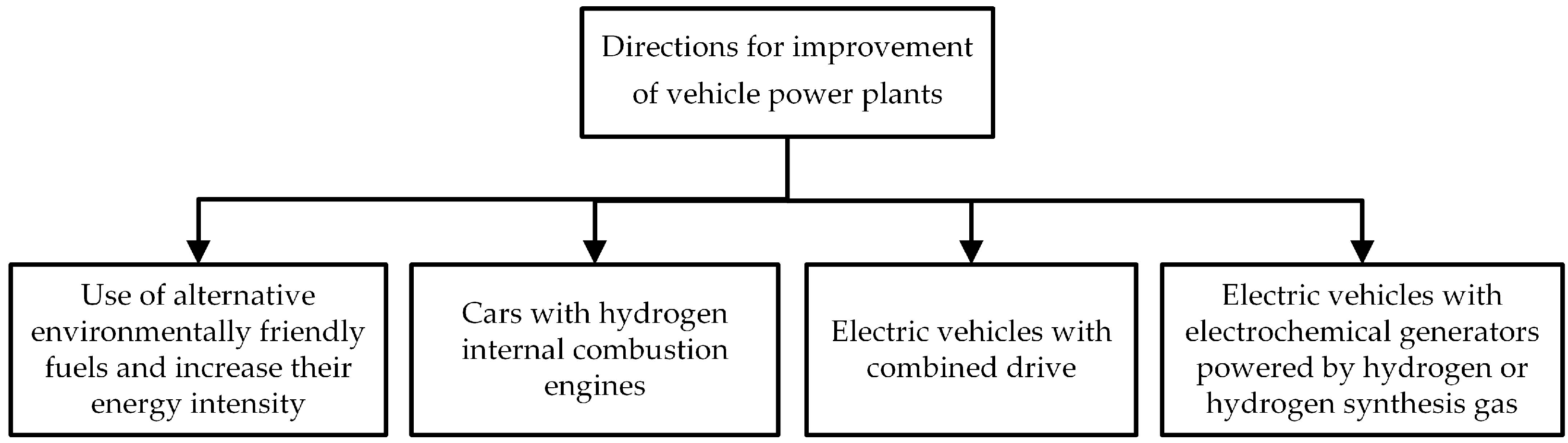
The global shortage of oil and environmental problems determine the importance of the application of more economical and ecological technologies in transport, including technologies for the improvement of power plants as the most energy-intensive vehicle component. Lutsyk et al. [45] considered four main areas of improvement of vehicle power plants, which are presented in Figure 2.

One of the solutions to the environmental crisis and dependence on oil is the transition from vehicles with an internal combustion engine to electric vehicles: battery electric vehicles (BEVs), hybrid electric vehicles (HEVs), plug-in hybrid electric vehicles (PHEVs), and fuel cell electric vehicles (FCEVs). Energy consumption assessment tools are needed to compare the different types of electric vehicles and manage them optimally.

According to the authors in [45], the most promising energy source is hydrogen, which can increase the efficiency of an internal combustion engine by 1.7 times compared to a conventional gasoline engine. An efficient way to use hydrogen is to use a fuel cell electric vehicle (FCEV). Hissler [46] distinguishes three categories of FCEVs: mild hybridization, mid-power, and range extender. In the first case, the only source of energy is hydrogen. In this case, a small capacity buffer battery is used only at high voltage. FCEVs in the second category use hydrogen and a battery to power the drivetrain. In the FCEV of the third category, the energy demand is provided by the battery. A fuel cell is only used when needed: to charge the battery or increase energy. Auxiliary elements such as pumps, compressors, and cooling components affect the efficiency of the fuel cell system. In work [46], Hissler gives three methods for determining hydrogen consumption according to ISO 23828 [47]: the pressure method based on the measurement of pressure and temperature; the gravimetric method based on the measurement of the mass of the tank; and the flow method based on the measurement of the amount of hydrogen. Hissler defines the total energy demand E_cycle (Ws) in the WLTC cycle using the following formula:

$$E_{cycle}={\displaystyle \sum }_{t_{start}+1}^{t_{end}}{E}_i$$

(25)

where E_i = F_i ×d_i for F_i > 0 and E_i = 0 for F_i ≤ 0; d_i is the distance traveled during test cycle i, km.

$$F_i=F_0+F_1\frac{v_i+v_{i-1}}{2}+F_2{\left(\frac{v_i+v_{i-1}}{2}\right)}^2+1.03\times TM\times a_i$$

(26)

where F_i is the driving force during time period (i − 1) to (i), N; v_i is the target velocity at time t_i, km/h; TM is the test mass, kg; a_i is the acceleration during time period (i − 1) to (i), m/s²; and F₀ F₁ and F₂ are the road load coefficients for the test vehicle under consideration in N, N/km/h and in N/(km/h)², respectively.

In work [48], Usmanov investigates the existing strategies for the energy consumption management of HEVs. The strategies aim to distribute power between energy sources to maintain battery charge and minimize energy consumption and emissions. The author divides all strategies into two groups: those based on rules and those based on optimization. Each strategy corresponds to a set of defined models. Rule-based strategies use deterministic models or fuzzy logic (default, adaptive, predictive).

Martyushev et al. systematized methods for increasing the energy efficiency of BEVs, PHEVs, and FCEVs based on the optimization of battery consumption [49]. Individual and public transport were the subjects of the investigation. The authors in [49] divided the studied methods into groups (Figure 3).

The most effective methods are defined in each group. Each method is only used for a given electric vehicle type. These methods use physical laws to estimate energy consumption. The dynamics of energy consumption is studied on the basis of simulation models, neural networks with deep learning algorithms, genetic algorithms, fuzzy logic models, optimization models of dynamic programming, forecasting models, PTV VISSIM models, and hybrid models. In general, the list of these models is consistent with the mathematical models considered in [48].

The fuzzy logic-based models were applied in control units of auxiliary systems of hybrid cars and fuel cell hybrid vehicles in works [50,51,52]. Neural networks and genetic algorithms for estimating fuel consumption were investigated in [53,54]. The authors of [54] study the methods for predicting the operation of supercapacitors. Supercapacitors can be used as an additional power source for starting EVs. They provide the advantages of long life and environmental protection. The electrochemical system in the supercapacitor has strong characteristic connections. This complicates the application of their physical models and gives priority to the model-based methods for predicting the performance parameters of supercapacitors. The HHO algorithm is used to optimize the initial learning speed and structure of the hidden layer of the network and is based on the definition of the escape energy factor. To confirm the high performance of the HHO-LSTM algorithm, the authors used various capacitor sets to predict their capacitance. The authors predicted the supercapacitors’ capacity attenuation under various temperature conditions.

Paper [55] examines the advantages and limitations of methods for estimating battery parameters that correlate with SOC and SOH values. These methods are implemented on the basis of sensor systems. Non-embedded and embedded sensors are used to measure current, voltage, temperature on the surface and inside the battery, and strain and stress in the working process. Among these parameters, temperature and strain have the greatest impact on SOC. The paper proves the prospects of using non-embedded and embedded fiber optic sensors for SOC evaluation. Special attention is paid to optical fiber grating sensors (TFBG, FPI) and optical fiber evanescent wave (OFEW, SPR, LSPR). However, it is noted that there is no connection between fiber optic sensors and battery management system algorithms. This determines the directions of future research in this field.

Systematization of the main considered energy efficiency assessment models and their sub-models for determining fuel/energy consumption is presented in the next section. The existing methods of energy efficiency assessment are based on static arrays of input data of constant dimensions (an unchanged list of parameters). Section 3.2 presents a method for predicting the vehicle energy efficiency based on dynamic arrays of input data (with variable dimensions) depending on the current state of the transport system.

3. Results

3.1. Systematization of the Considered Models for Controlling the Vehicle Energy Efficiency in Intelligent Transport Systems

Table 5. Peculiarities of mathematical methods and models for estimating fuel/energy consumption.

Source	Study Object Location	Units	Short Characteristic	Limitations and Disadvantages
[17]	China	L/100 km	Fuel consumption is estimated at constant speeds for commercial trucks; the use of the Top Runner method made it possible to perform a new classification of vehicles within one weight category	The model requires the use of additional methods for determining the fuel consumption rate (L/km) in countries where there is no corresponding standard; the correction coefficient is determined under the condition of nominal loading
[22]	Poland	g/s, g	The method is implemented by means of statistical analysis; allows study of the influence of stop time, peak hours, and other vehicle traffic conditions on fuel consumption in the urban driving cycle	Requires high-precision means of measuring speed and acceleration; does not take into account changes in passenger traffic on the route during the day
[29]	Ukraine	g/km, g/s	Separate models are used, taking into account the modes of movement: steady movement, acceleration mode, idling	Models take into account only parameters of vehicles
[30]	USA (Tennessee, Ohio, Michigan)	L/s	The models estimate the fuel consumption of stabilized vehicles in a hot state	The need to use a dynamometric stand for calibration of regression coefficients
[31]	USA, Qatar	L/s	A complex model is used for different acceleration ranges; high modeling accuracy is achieved at high speeds of vehicles	Similar to [30]
[32]	Poland	L/(pass∙km), L	The model is built for city buses of a large class in the local driving cycle and allows estimation of fuel consumption on individual sections of the route	The absolute values of fuel consumption (L) contain an error of about 10% when increasing the distance of technical mileage
[33]	China	g/person, L/100 km, L/(per 100 km)	The VSP model includes road load coefficients that take into account the type of vehicle; the method is applied to compare the efficiency of a bus and a passenger car on an urban route based on the fuel ratio, L/(per 100 km)	Statistical data for comparing the effectiveness of vehicles were measured in time intervals that do not coincide with different categories of vehicle; collection was carried out via mobile phone due to lack of GPS devices
[34]	Portugal	g/s	The model is built on the basis of certified data for 3 European driving cycles with subsequent correction of the fuel consumption estimate of EURO 5 vehicles using road data that take into account real conditions outside the cycle	Necessity of using on-board diagnostics port reader from OBDKey and GPS receiver
[37]	Ukraine	g/s	The possibility of using the CMEM model for modeling the consumption of diesel biofuel and alternative fuels	Requires special software and access to relevant databases; the value of some parameters in CMEM was taken by default due to the complexity of their determination
[38]	Austria	g/s, L/100 km or kg/100 km	The simulation program is made in Simulink using MATLAB and calculates fuel consumption every 100 milliseconds; the application of the adapted powertrain model ensured that characteristic maps were calculated through traction force and speed instead of torque and engine speed	To determine the mass flow of air, a thermofilm air mass sensor is required; to calculate mass emissions in real conditions, it is necessary to equip the car with an on-board measuring device; transverse dynamics were not taken into account in the modeling; for heavy duty vehicles, the developed model gave an error of about 10%
[39]	USA (Utah)	g/s	Allows determination of the optimal signal synchronization plan based on the criterion of fuel consumption (emissions) due to the integration of VISSIM, CMEM, and VISGAOST using a genetic algorithm	The accuracy of the result depends on the quality of modeling and the methodology that describes the movement of vehicles. Models and their calibration require a large amount of data; statistical data were obtained in good weather and dry conditions; optimization requires significant time resources
[40]	Sweden	L/km	Linear dependences of fuel consumption growth on the growth of each of the road parameters were obtained; the estimation of fuel consumption is determined on the basis of a nonlinear function that takes into account a wide range of road parameters; allows use of research results in the construction of new roads to achieve energy savings when using fuel	Only investigates the impact of road characteristics and track options on fuel consumption
[44]	USA (the state of Arizona)	gal/100 mi	The flexibility of the simulation model is ensured by the possibility of adding and subtracting attributes to increase the level of accuracy; the GPS trajectory of the vehicle is determined as significant attribute in addition to speed and gradient	The methodology requires a large amount of real driving data and filtering to eliminate the measurement error of GPS devices; the energy estimation model showed less accuracy than the FASTSim model, but it accurately determined the route with the least fuel/energy consumption
[46]	France	Ws	Hydrogen measurement methods comply with the ISO standard; the measurement of energy consumption was carried out without taking into account the operation of auxiliary components and systems	The hydrogen measuring device must provide an accuracy of +(−)1% of the mass of consumed hydrogen; application of the flow method requires a flowmeter that must be calibrated and a device to reduce pulsation to improve measurement accuracy
[50]	Italy	L/100 km	Various FCEV power consumption management strategies have been applied, the best of which provide fuel cell system efficiency of over 33%; the effectiveness of the strategy is determined by fuel consumption based on five driving cycles; the model takes into account the influence of auxiliary systems	The results were obtained under conditions of certified driving cycles
[56]	Italy	L/vehicle-km	The developed simulation models can be used for other spatial scales and countries; the level of hydrogen consumption is estimated according to the linear trend of FCEV entering the flow of heavy-duty transport based on the flow matrix	The use of FCEVs is limited to domestic transport; the study assumes an uncongested network

gives a brief description of the features of the application of the models and methods of fuel and energy consumption of vehicles.

Table 6. Fuel/energy consumption models and their parameters.

Source	Parameter Group					Model
	Vehicle Technology	Vehicle Operating	Road	Traffic Environment	Traffic Flow
[22]	×	√	√	×	×	Function of the VSP index
[29]	√	√	×	×	×	Polynomials of the 2nd and 3rd degrees
[30]	√	√	×	√	√	Polynomial of the 3rd degree, logarithmic dependences
[31]	√	√	×	√	×	Exponential regression
[32]	×	√	×	×	×	Hyperbolic regression
[33]	√	√	√	√	×	Function of the VSP index
[34]	√	√	√	×	×	A piecewise-defined nonlinear function for the 3 different VSP modes
[37]	√	√	√	√	×	Complex modal model of SMEM; carbon balance models for gasoline and diesel vehicles
[38]	√	√	√	×	×	Dependence on speed and acceleration by the method to generate fuel consumption maps; carbon balance model for CNG vehicle; linear function of the vehicle speed and the traction force
[39]	√	√	√	×	√	VISSIM model and CMEM model integrated with VISGAOST program
[40]	×	√	√	√	×	Multiple nonlinear regression
[17]	×	√	×	×	×	The model based on the constant speed fuel consumption method
[44]	×	√	√	×	√	Vehicle powertrain simulation model performed in The Future Automotive Systems Technology Simulator (FASTSim); a prediction model based on a multidimensional lookup table of fuel/energy consumption
[46]	√	√	√	×	×	Simulink model
[56]	×	√	×	√	√	Simulation models; linear trends
[50]	√	√	×	×	×	Quasi-static model made by the Advisor, MATLAB; fuzzy logic-based energy management model

√: a group of parameters is taken into account in the model, ×: a group of parameters is not taken into account in the model.

and

Table 7. Classification of methods for estimating vehicle fuel/energy consumption of a given category.

Vehicle Category	Power Plant	Source
M1	Petrol	[29,30,31,33,37,40,44]
	Diesel	[29,30,31,33,37,40]
	Gas	[29,38]
	Battery	[9] (the source contains links to 81 models)
	Hybrid	[44,46,49,51,52]
	Fuel Cell	[46]
M2	Petrol	[29]
	Diesel	[29]
	Gas	[29]
M3	Petrol	[29,33,34]
	Diesel	[22,29,32,33,34]
	Gas	[29]
	Battery	[9] (the source contains links to 81 models), [49]
	Fuel Cell	[49,50]
N1	Petrol	[29,30,31,39]
	Diesel	[29,30,31]
	Gas	[29]
N2	Petrol	[17,29,37,40]
	Diesel	[17,29,37,39,40]
	Gas	[29]
	Fuel Cell	[49,56]
N3	Petrol	[17,29,40]
	Diesel	[17,29,39,40]
	Gas	[29]
	Fuel Cell	[49,56]

supplement it. Table 6 shows the main types of mathematical models and defines the groups of their parameters. In Table 7, references to used sources are distributed by vehicle category, taking into account the type of power plant. The vehicle categories are adopted according to the Rules and Directives of the European Union (EU) and the United Nations Economic Commission for Europe (UNECE).

In the generalized Table 7 and

Table 8. Classification of energy efficiency assessment methods for vehicles with conventional and alternative energy plants.

Vehicle Category	Power Plant	Calculation Formula	Source
M1	Petrol	(1), (7), (9)	[1,14,20,22,28]
	Diesel	(1), (7), (9)	[1,14,20,22,28]
	Gas	(1), (7)	[1,14,20,22]
	Battery	(7)	[20,22]
	Hybrid	(7)	[20,22]
	Fuel Cell	(7)	[20,22]
M2	Petrol	(1), (7)	[1,14,20,22]
	Diesel	(1), (7)	[1,14,20,22]
	Gas	(1), (7)	[1,14,20,22]
	Battery	(7)	[20,22]
	Hybrid	(7)	[20,22]
	Fuel Cell	(7)	[20,22]
M3	Petrol	(1), (7)	[1,14,20,22]
	Diesel	(1), (6), (7), (8)	[1,14,20,22]
	Gas	(1), (7)	[1,14,20,22]
	Battery	(7)	[20,22]
	Hybrid	(7)	[20,22]
	Fuel Cell	(7)	[20,22,50]
N1	Petrol	(1), (5), (7)	[1,14,19,20,22]
	Diesel	(1), (5), (7)	[1,14,19,20,22]
	Gas	(1), (7)	[1,14,20,22]
	Battery	(7)	[20,22]
	Hybrid	(7)	[20,22]
	Fuel Cell	(7)	[20,22]
N2	Petrol	(1), (4), (5), (7)	[1,14,17,18,19,20,22]
	Diesel	(1), (4), (5), (7)	[1,14,17,18,19,20,22]
	Gas	(1), (7)	[1,14,20,22]
	Battery	(7)	[20,22]
	Hybrid	(7)	[20,22]
	Fuel Cell	(7)	[20,22,50]
N3	Petrol	(1), (4), (5), (7)	[1,14,17,18,19,20,22]
	Diesel	(1), (2), (3), (4), (5), (7)	[1,14,16,17,18,19,20,22]
	Gas	(1), (7)	[1,14,20,22]
	Battery	(7)	[20,22]
	Hybrid	(7)	[20,22]
	Fuel Cell	(7)	[20,22,50]

, the distribution of references’ sources for the considered model types is made based on the convenience of their selection for evaluating the vehicle energy efficiency in intelligent transport systems.

From the analysis of Table 5, Table 6, Table 7 and Table 8, it is possible to identify groups of methods that were not given enough attention in this study. Generalized information on evaluation methods is useful when using the specified models in intelligent transport management systems. It is convenient to determine the method for estimating fuel/energy consumption taking into account the category of vehicle and the type of power plant. If there are several methods, an additional selection criterion should be used, for example, the research object location or the model accuracy.

3.2. Evaluation of the Energy Efficiency of Vehicles Based on the 3D Morphological Model of the Transport System

Internal and external factors affect the energy efficiency of vehicles. Table 5 shows the main groups of factors influencing fuel/energy consumption. The functional elements of the transport system are formed on the basis of these groups, in particular, the structure of transport energy efficiency control subsystem (TrEECS) [1,14]. It is convenient to represent the morphological structure of the TrEECS in the form of a matrix (Figure 4).

The functional elements (beige cells in the figure) are characterized by morphological features x_j (green cells). Morphological features correspond to the parameters of the system. Each feature has a domain of admissible values x_ji (options of implementation), blue cells. A set of implementation options forms a certain configuration of the system (dark blue cells). The given configuration is a dynamic array, the size of which varies according to the current values of the system parameters. Individual cells in different morphological matrices may coincide in meaning. We will call such cells key fields (foreign keys). A specific configuration of a transport system can be extended by the configuration of other systems through external keys. For example, the functional element “infrastructure” of the transport system is connected to the functional element “autoservice enterprise” of the car service system by the key “gas/charging stations”. In this way, the 3D matrix is formed (Figure 4).

The authors in [1] present a mathematical transformation of the classic morphological model into a fuzzy rule base for evaluating, controlling, and forecasting the energy efficiency of vehicles. This transformation cannot be implemented for the TrEECS 3D model. A solution to this issue is the use of the TrEECS object database. The optimal configuration of the system can be determined by solving the optimization problem according to the criterion of energy efficiency of the vehicle (Figure 5)

Figure 5 uses the following notation: X* is the optimal system morphological structure; Ie* is the value of the energy efficiency indicator under the condition of optimal system morphological structure.

This process is iterative. On the basis of the configurations and indicators of the lower levels of the TrEECS, it is possible to form the objects and indicators of the system’s upper level.

A partial case of the TrEECS morphological matrix is the 2D model. This model was tested in works [1,13,14] on the example of 25 sections of transport networks in Poland and Ukraine. Mathematical models were built on the basis of the morphological model. This made it possible to investigate the influence of the system parameters on the energy efficiency of 16 vehicles of six categories (Table 8) with the studied power plants. The relative standard deviation was 1.2% for the TrEECS fuzzy logic model, 1.3% for the neural network model, and 1.5% for the TrEECS multiple regression. Approbation of the 3D model will be performed in further studies.

4. Discussion

The paper examines the main methods and models of energy efficiency assessment from the perspective of the possibility of their application in intelligent transport systems and the selection of the optimal vehicle technology. Despite the large number of studies in this area, the main part of the applied models only concerns a certain set of transport technologies. Little attention is paid to the development of universal methods. Not all models take into account the main range of transport system parameters for evaluating the vehicle efficiency. Within the framework of this study, an attempt was made to systematize the methods of estimating the fuel and energy consumption of vehicles with various power plants at the stage of operation. Fuel/energy consumption models of vehicles are components of the majority of vehicle energy efficiency models. The performed systematization allowed the identification of combinations of vehicle category and power plant types for which energy efficiency and fuel/energy consumption models were not sufficiently investigated. Therefore, the work in the direction of the research of energy efficiency evaluation methods will continue in the future, and the research focus will be on the efficiency models of vehicles with alternative power plants. In addition, this work determined the energy efficiency at the stage of motor vehicle operation. In the future, it an investigation of this issue is planned to be carried out at the stages of production and disposal of vehicles.

The vehicle is considered a functional element of the transport system that interacts with its other elements. Based on the results of the work, five main groups of factors influencing the vehicle energy efficiency were identified: vehicle technical features, vehicle operating characteristics, road, traffic environment, and traffic flow. These groups were selected as functional elements of the transport energy efficiency control subsystem (TrEECS) in the intelligent transport system. A significant group of researchers single out the driving style as an element of influence on the vehicle energy efficiency. Therefore, it the investigation of driving parameters is planned and these parameters will be added to the system morphological model. The elements of the transport system can be part of other systems. This feature was used to build the concept of a 3D morphological model. This model was obtained on the morphological structure of the basis of the transport system, to which parameters of conjugated morphological structures were added. In this case, the transition from a morphological model to a mathematical one is difficult. One of the directions of further research is the development of an alternative system object model and a module for choosing a method of evaluating the vehicle energy efficiency under given operating conditions. The analysis of the scientific sources showed that the vehicle energy efficiency can be a criterion for optimizing other system elements, particularly roads. Therefore, the system configuration is not static. It is recommended that the system be periodically improved according to the optimization algorithm (Figure 5). When forming a morphological model, only independent parameters of the system should be taken into account. For this, the Farrar–Glober algorithm should be used. The scheme of the algorithm is presented in [14]. It is better to calculate the energy efficiency indicator according to formula (7). This indicator is universal. To calculate its denominator, it is necessary to select a method for estimating energy/fuel consumption. At the same time, it is advisable to use Table 5, Table 6 and Table 7.

The presented mathematical models of energy efficiency, fuel consumption and energy consumption, the concept of a 3D morphological model, and an algorithm for optimizing the transport system according to the energy efficiency criterion can be useful for system analysts and designers of intelligent transport systems, as well as for improving the structural elements of the transport system.

5. Conclusions

• The evaluation of vehicle energy efficiency is used in the supervision and control processes in intelligent transport systems. The analysis of work in the field of vehicle energy efficiency showed that most of the methods for its evaluation can only be applied for certain types of vehicles. The choice of method must be made based on the purpose of the research and an analysis of the limitations of the existing methods.
• The classification of methods for evaluating the energy efficiency of vehicles has been carried out. Four main groups of these methods are distinguished: measuring the vehicle fuel efficiency for given driving cycles, energy consumption analysis, the WTW analysis, and evaluating the energy efficiency throughout the entire LCA. The methods from the first three groups can determine partial estimates of energy efficiency for use by the methods of the fourth group. Many methods lead to narrowing the field of research to the consideration of energy efficiency assessment methods at the stage of operation in the life cycle of vehicles.
• The main attention in the work is given to the review of mathematical models of energy efficiency indicators of vehicles. The most universal model defines the ratio of useful work to spent energy. This assessment takes into account the design and operational characteristics of the vehicle, the parameters of the road and the environment. Other transport system parameters can be considered in partial energy/fuel consumption models. This makes it possible to use a single energy efficiency criterion for different categories of vehicles with conventional and alternative energy plants. The paper systematizes the models of fuel consumption and energy consumption of vehicles at the stage of operation. The advantages and limitations of these models, the location of the research object, and the necessary technical means are highlighted. This will help researchers choose an adequate model for the given task.
• The main groups of factors influencing the energy efficiency of vehicles are highlighted. On the basis of these, the concept of a 3D morphological model is presented. Its use allows the dynamic expansion of the parameter sets of system objects. The morphological model is conceptual. In order to display it at the logical and physical levels, it is proposed that the object model of the transport system is used. These models and the energy efficiency criterion are the basis of the given algorithm for optimizing the elements of the transport system. The paper provides recommendations for the application of this algorithm.

References

1. Mateichyk, V.; Kostian, N.; Smieszek, M.; Mosciszewski, J.; Tarandushka, L. Evaluating Vehicle Energy Efficiency in Urban Transport Systems Based on Fuzzy Logic Models. Energies 2023, 16, 734. [Google Scholar] [CrossRef]
2. Volkov, V.P.; Vilskyi, H.B. Teoriia Rukhu Avtomobilia (Car Motion Theory); VTD “Universytetska Knyha”: Sumy, Ukraine, 2021; 320p. (In Ukrainian) [Google Scholar]
3. Mediouni, H.; Ezzouhri, A.; Charouh, Z.; El Harouri, K.; El Hani, S.; Ghogho, M. Energy Consumption Prediction and Analysis for Electric Vehicles: A Hybrid Approach. Energies 2022, 15, 6490. [Google Scholar] [CrossRef]
4. Huertas, J.I.; Giraldo, M.; Quirama, L.F.; Díaz, J. Driving Cycles Based on Fuel Consumption. Energies 2018, 11, 3064. [Google Scholar] [CrossRef]
5. Achour, H.; Olabi, A.G. Driving cycle developments and their impacts on energy consumption of transportation. J. Clean. Prod. 2016, 112, 1778–1788. [Google Scholar] [CrossRef]
6. André, M.; Joumard, R.; Vidon, R.; Tassel, P.; Perret, P. Real-world European driving cycles, for measuring pollutant emissions from high- and low-powered cars. Atmos. Environ. 2006, 40, 5944–5953. [Google Scholar] [CrossRef]
7. Ho, S.; Wong, Y.; Chang, V.W. Developing Singapore Driving Cycle for passenger cars to estimate fuel consumption and vehicular emissions. Atmos. Environ. 2014, 97, 353–362. [Google Scholar] [CrossRef]
8. Hung, W.T.; Tong, H.Y.; Lee, C.P.; Ha, K.; Pao, L.Y. Development of a practical driving cycle construction methodology: A case study in Hong Kong. Transp. Res. Part D 2007, 12, 115–128. [Google Scholar] [CrossRef]
9. Chen, Y.; Wu, G.; Sun, R.; Dubey, A.; Laszka, A.; Pugliese, P. A Review and Outlook of Energy Consumption Estimation Models for Electric Vehicles. SAE J. STEEP 2021, 2, 79–96. [Google Scholar] [CrossRef]
10. Sun, D.J.; Zheng, Y.; Duan, R. Energy consumption simulation and economic benefit analysis for urban electric commercial-vehicles. Transp. Res. Part D 2021, 101, 103083. [Google Scholar] [CrossRef]
11. Kambly, K.R.; Bradley, T.H. Estimating the HVAC energy consumption of plug-in electric vehicles. J. Power Sources 2014, 259, 117–124. [Google Scholar] [CrossRef]
12. Lee, J.T.; Kwon, S.; Lim, Y.; Chon, M.S.; Kim, D. Effect of Air-Conditioning on Driving Range of Electric Vehicle for Various Driving Modes; SAE Technical Paper; SAE International: Warrendale, PA, USA, 2013. [Google Scholar] [CrossRef]
13. Mateichyk, V.; Smieszek, M.; Kostian, N. Evaluation of transport system configuration by efficiency indicators. TT 2022, 2022, 52–62. [Google Scholar] [CrossRef]
14. Smieszek, M.; Kostian, N.; Mateichyk, V.; Mościszewski, J.; Tarandushka, L. Determination of the Model Basis for Assessing the Vehicle Energy Efficiency in Urban Traffic. Energies 2021, 14, 8538. [Google Scholar] [CrossRef]
15. Norms of Fuel and Lubricants Consumption in Road Transport: Order of the Ministry of Transport of Ukraine 10.02.1998 No. 43 as Amended in 2012. Available online: https://zakon.rada.gov.ua/rada/show/v0043361-98#n12 (accessed on 30 June 2023). (In Ukrainian)
16. Gritsuk, I.; Volkov, V.; Majak, M.; Ukrainskyi, Y.; Volodarets, M.; Volkova, T.; Ryzhova, V. Formation of the Method of ensuring the Rating of indicators and management of the Fuel economy of the Vehicle in variable operating conditions. Adv. Mech. Eng. Transp. 2022, 18, 56–65. (In Ukrainian) [Google Scholar] [CrossRef]
17. Tian, J.; Yang, D.; Zhang, H.; Liu, L. Classification method of energy efficiency and CO2 emission intensity of commercial trucks in China’s road transport. Procedia Eng. 2016, 137, 75–84. [Google Scholar] [CrossRef]
18. Khabutdinov, R.A.; Kovbasenko, O.G. Technique of the analysis of exploitation-technological and energy indexes of truck trailer. Bull. Natl. Transp. Univ. Part 2 Part 1 Ser. “Tech. Sci.” 2014, 29, 331–338. [Google Scholar]
19. Khabutdinov, R.A. System concept of energy-resource synergy and methodology of technological-innovative management on motor transport. Bull. Natl. Transp. Univ. 2020, 1, 365–374. (In Ukrainian) [Google Scholar] [CrossRef]
20. Kostian, N.L. Complex energy efficiency evaluation of urban passenger transport. Bull. Natl. Transp. Univ. 2022, 3, 178–185. (In Ukrainian) [Google Scholar] [CrossRef]
21. Khabutdinov, R.A.; Fedorenko, I.O. Analysis of the impact of transport energy efficiency indicators of the bus for urban passenger transportation. Sci. Notes V.I. Vernadsky Taurida Natl. Univ. Ser. Tech. Sci. 2021, 32, 259–266. (In Ukrainian) [Google Scholar] [CrossRef]
22. Smieszek, M.; Mateichyk, V. Determining the fuel consumption of a public city bus in urban traffic. In IOP Conference Series: Materials Science and Engineering, Proceedings of the 26th International Slovak-Polish Scientific Conference on Machine Modelling and Simulations (MMS 2021), Bardejovské Kúpele, Slovakia, 13–15 September 2021; IOP Publishing Ltd.: Bristol, UK, 2021; p. 1199. [Google Scholar] [CrossRef]
23. Kim, J.J.; Kim, J.; Hann, T.; Kim, D.; Roh, H.S.; Lee, S.J. Considerable drag reduction and fuel saving of a tractor–trailer using additive aerodynamic devices. J. Wind Eng. Ind. Aerodyn. 2019, 191, 54–62. [Google Scholar] [CrossRef]
24. Mosiężny, J.; Ziegler, B.; Grzymisławski, P.; Ślefarski, R. Base drag reduction concept for commercial road vehicles. Energy 2020, 205, 118075. [Google Scholar] [CrossRef]
25. Rievaj, V.; Stopka, O.; Vrábel, J.; Mokrickova, L.; Schmidt, C. The Impact of Air Resistance on the Fuel Consumption in Real Conditions within the Transport Operation. Commun.-Sci. Lett. Univ. Zilina 2016, 18, 57–61. [Google Scholar] [CrossRef]
26. Jo, S.; Kim, H.J.; Kwon, S.I.; Lee, J.T.; Park, S. Assessment of Energy Consumption Characteristics of Ultra-Heavy-Duty Vehicles under Real Driving Conditions. Energies 2023, 16, 2333. [Google Scholar] [CrossRef]
27. Mateichyk, V.; Soltus, A.; Klimov, E.; Kostian, N.; Smieszek, M.; Kovbasenko, S. Regularities of Changes in the Motion Resistance of Wheeled Vehicles along a Curvilinear Trajectory. Machines 2023, 11, 570. [Google Scholar] [CrossRef]
28. Podrigalo, M.A.; Abramov, D.V.; Tarasov, Y.V.; Kholodov, M.P.; Kaidalov, R.O.; Podrigalo, N.M.; Shein, V.S. Improvement evaluation methodology of vehicle load and energy efficiency. Automob. Transp. 2021, 49, 36–44. [Google Scholar] [CrossRef]
29. Dmytriiev, M.M. M 218-02070915-694:2011 Methods for Assessing the Ingredient and Parametric Pollution of the Roadside Environment by the System Traffic Flow—Road; National Transport University: Kyiv, Ukraine, 2011; p. 28. [Google Scholar]
30. Ahn, K.; Rakha, H.; Trani, A.; Van Aerde, M. Estimating vehicle fuel consumption and emissions based on instantaneous speed and acceleration levels. J. Transp. Eng. 2002, 128, 182–190. [Google Scholar] [CrossRef]
31. Du, J.; Rakha, H.A.; Filali, F.; Eldardiry, H. COVID-19 pandemic impacts on traffic system delay, fuel consumption and emissions. Int. J. Transp. Sci. Technol. 2021, 10, 184–196. [Google Scholar] [CrossRef]
32. Smieszek, M.; Kostian, N.; Mateichyk, V.; Mosciszewski, J.; Tarandushka, L. Estimation of the Public Transport Operating Performance: Example of a Selected City Bus Route. Commun.-Sci. Lett. Univ. Zilina 2023, 25, B7–B21. [Google Scholar] [CrossRef]
33. Chen, X.; Shan, X.; Ye, J.; Yi, F.; Wang, Y. Evaluating the Effects of Traffic Congestion and Passenger Load on Feeder Bus Fuel and Emissions Compared with Passenger Car. Transp. Res. Procedia 2017, 25, 616–626. [Google Scholar] [CrossRef]
34. Duartea, G.; Gonçalvesa, G.; Farias, T. A methodology to estimate real-world vehicle fuel use and emissions based on certification cycle data. Procedia-Soc. Behav. Sci. 2014, 111, 702–710. [Google Scholar] [CrossRef]
35. Macor, A.; Rossetti, A. Fuel consumption reduction in urban buses by using power split transmissions. Energy Convers. Manag. 2013, 71, 159–171. [Google Scholar] [CrossRef]
36. Zhou, M.; Jin, H.; Wang, W. A review of vehicle fuel consumption models to evaluate eco-driving and eco-routing. Transp. Res. Part D Transp. Environ. 2016, 49, 203–218. [Google Scholar] [CrossRef]
37. Kolodnytska, R.V. Modeling of fuel consumption for road transport, taking into account transport technologies. Sci. Notes V.I. Vernadsky Taurida Natl. Univ. Ser. Tech. Sci. 2022, 33, 201–208. [Google Scholar] [CrossRef]
38. Cachón, L.; Pucher, E. Fuel Consumption Simulation Model of a CNG Vehicle Based on Real-World Emission Measurement; SAE Technical Paper; SAE International: Warrendale, PA, USA, 2007. [Google Scholar] [CrossRef]
39. Stevanovic, A.; Stevanovic, J.; Zhang, K.; Batterman, S. Optimizing traffic control to reduce fuel consumption and vehicular emissions. Transp. Res. Rec. 2009, 2128, 105–113. [Google Scholar] [CrossRef]
40. Carlson, A.; Hammarström, U.; Eriksson, O. Models and Methods for the Estimation of Fuel Consumption due to Infrastructure Parameters. Deliverable 2.1 in MIRAVEC—Modelling Infrastructure Influence on Road Vehicle Energy Consumption, Project No. 832615, ERA NET Road. 2013. Available online: https://trimis.ec.europa.eu/sites/default/files/project/documents/03_miravec_d2.1_v5.0.pdf (accessed on 10 June 2023).
41. Carlson, A.; Karlsson, R.; Eriksson, O. Energy Use Due to Traffic and Pavement Maintenance: The Cost Effectiveness of Reducing Rolling Resistance, VTI Notat 9A-2016; Statens Väg-Och Transportforskningsinstitut: Linköping, Sweden, 2016; p. 84. Available online: https://www.diva-portal.org/smash/get/diva2:925846/FULLTEXT01.pdf (accessed on 10 June 2023).
42. Carlson, A.; Vieira, T. The Effect of Water and Snow on the Road Surface on Rolling Resistance; Swedish National Road and Transport Research Institute (VTI): Linköping, Sweden, 2021. [Google Scholar] [CrossRef]
43. Wang, T.; Lee, I.-S.; Kendall, A.; Harvey, J.; Lee, E.-B.; Kim, C. Life cycle energy consumption and GHG emission from pavement rehabilitation with different rolling resistance. J. Clean. Prod. 2012, 33, 86–96. [Google Scholar] [CrossRef]
44. Holden, J.; Van Til, H.; Wood, E.; Zhu, L.; Gonder, J.; Shirk, M. Trip Energy Estimation Methodology and Model Based on Real-World Driving Data for Green-Routing Applications. Transp. Res. Rec. 2018, 2672, 41–48. [Google Scholar] [CrossRef]
45. Lutsyk, I.B.; Fendo, O.M.; Iskerskyi, I.S. Alternative power plants for vehicles. Energy Autom. 2014, 1, 75–82. [Google Scholar]
46. Hissler, C. How to Determine the Fuel Consumption for a Hydrogen Light Commercial Vehicle Project to Be Competitive? Master’s Thesis, KTH Royal Institute of Technology, Stockholm, Sweden, 2022. Available online: https://urn.kb.se/resolve?urn=urn:nbn:se:kth:diva-318825 (accessed on 30 June 2023).
47. ISO 23828:2022(E); Fuel Cell Road Vehicles—Energy Consumption Measurement—Vehicles Fuelled with Compressed Hydrogen. ISO: Geneva, Switzerland, 2022. Available online: https://cdn.standards.iteh.ai/samples/78416/c608ecee3d8747fa8274c552a153f9b4/ISO-23828-2022.pdf (accessed on 30 June 2023).
48. Usmanov, U. Review on Rule-Based Energy Management Strategies of Hybrid Electric Vehicles. Universum: Tech. Sci. 2022, 10, 57–61. Available online: https://7universum.com/ru/tech/archive/item/14386 (accessed on 30 June 2023). (In Russian).
49. Martyushev, N.V.; Malozyomov, B.V.; Khalikov, I.H.; Kukartsev, V.A.; Kukartsev, V.V.; Tynchenko, V.S.; Tynchenko, Y.A.; Qi, M. Review of Methods for Improving the Energy Efficiency of Electrified Ground Transport by Optimizing Battery Consumption. Energies 2023, 16, 729. [Google Scholar] [CrossRef]
50. Luciani, S.; Tonoli, A. Control Strategy Assessment for Improving PEM Fuel Cell System Efficiency in Fuel Cell Hybrid Vehicles. Energies 2022, 15, 2004. [Google Scholar] [CrossRef]
51. Lahlou, A.; Ossart, F.; Boudard, E.; Roy, F.; Bakhouya, M. A Real-Time Approach for Thermal Comfort Management in Electric Vehicles. Energies 2020, 13, 4006. [Google Scholar] [CrossRef]
52. Patrone, G.L.; Paffumi, E.; Otura, M.; Centurelli, M.; Ferrarese, C.; Jahn, S.; Brenner, A.; Thieringer, B.; Braun, D.; Hoffmann, T. Assessing the Energy Consumption and Driving Range of the QUIET Project Demonstrator Vehicle. Energies 2022, 15, 1290. [Google Scholar] [CrossRef]
53. Kanarachos, S.; Mathew, J.; Fitzpatrick, M. Instantaneous vehicle fuel consumption estimation using smartphones and Recurrent Neural Networks. Expert Syst. Appl. 2019, 120, 436–447. [Google Scholar] [CrossRef]
54. Ma, N.; Yin, H.; Wang, K. Prediction of the Remaining Useful Life of Supercapacitors at Different Temperatures Based on Improved Long Short-Term Memory. Energies 2023, 16, 5240. [Google Scholar] [CrossRef]
55. Yi, Z.; Chen, Z.; Yin, K.; Wang, L.; Wang, K. Sensing as the key to the safety and sustainability of new energy storage devices. Prot. Control Mod. Power Syst. 2023, 8, 27. [Google Scholar] [CrossRef]
56. Gallo, M.; Marinelli, M. The Impact of Fuel Cell Electric Freight Vehicles on Fuel Consumption and CO2 Emissions: The Case of Italy. Sustainability 2022, 14, 13455. [Google Scholar] [CrossRef]
Figure 1. Classification of vehicle fuel consumption models in terms of their transparency.
Energies 16 06331 g001
Figure 2. Promising directions of improvement of vehicle power plants [45].
Energies 16 06331 g002
Figure 3. Schematic grouping of the main methods to improve the energy efficiency of the electric vehicle [49].
Energies 16 06331 g003
Figure 4. Principle of building 3D morphological and object models of the transport system for evaluating and controlling the vehicle energy efficiency.
Energies 16 06331 g004
Figure 5. Algorithm for optimizing the transport system according to the criterion of energy efficiency of its elements.
Energies 16 06331 g005