
Remaining Useful Life Prediction of Lithium-Ion Batteries by Using a Denoising Transformer-Based Neural Network


Abstract
:1. Introduction
2. Literature Review
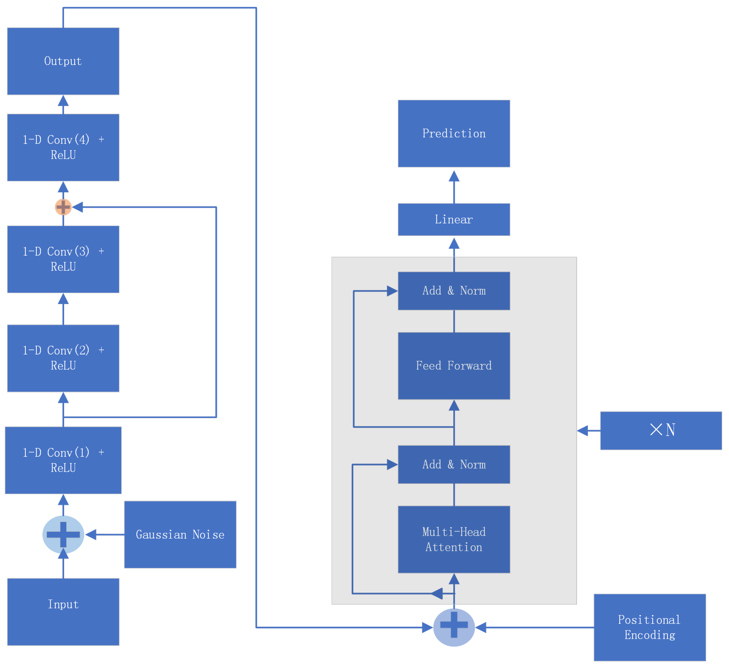
3. Methodology
3.1. Input Denoising
3.2. Transformer
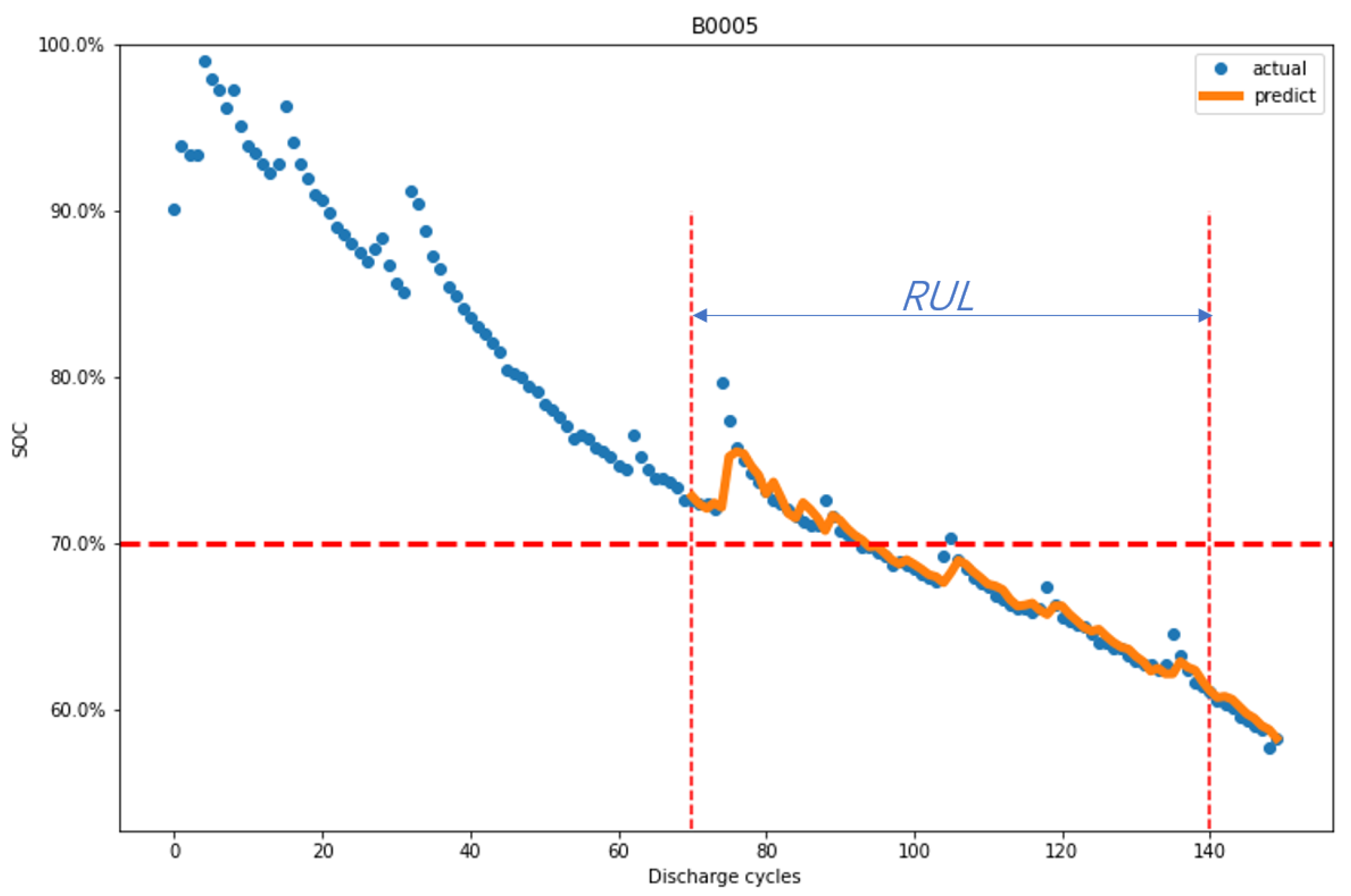
3.3. Prediction
3.4. Learning
3.5. Complexity Analysis of the DTNN Method
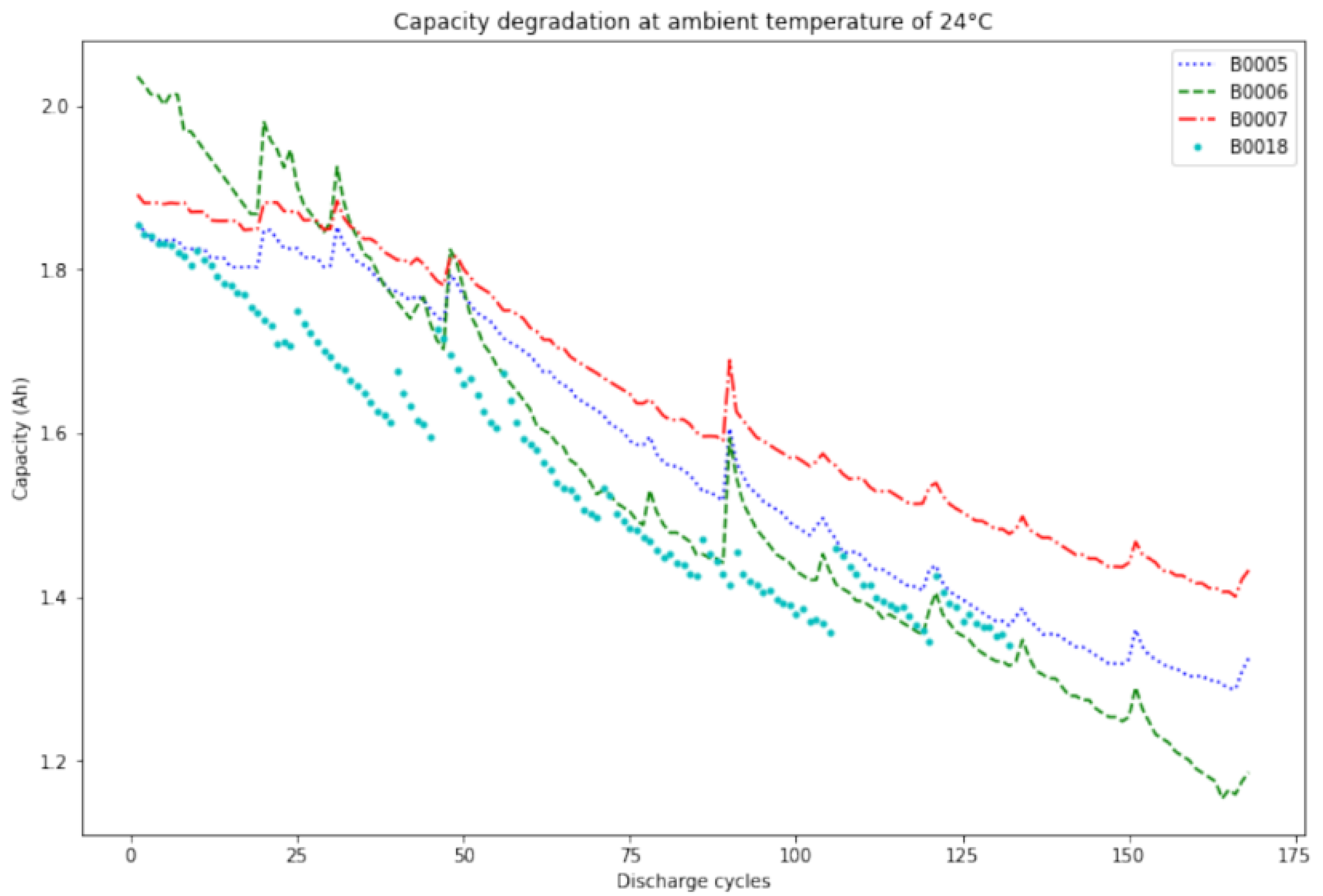
4. Experiment Setup
5. Experiment Result
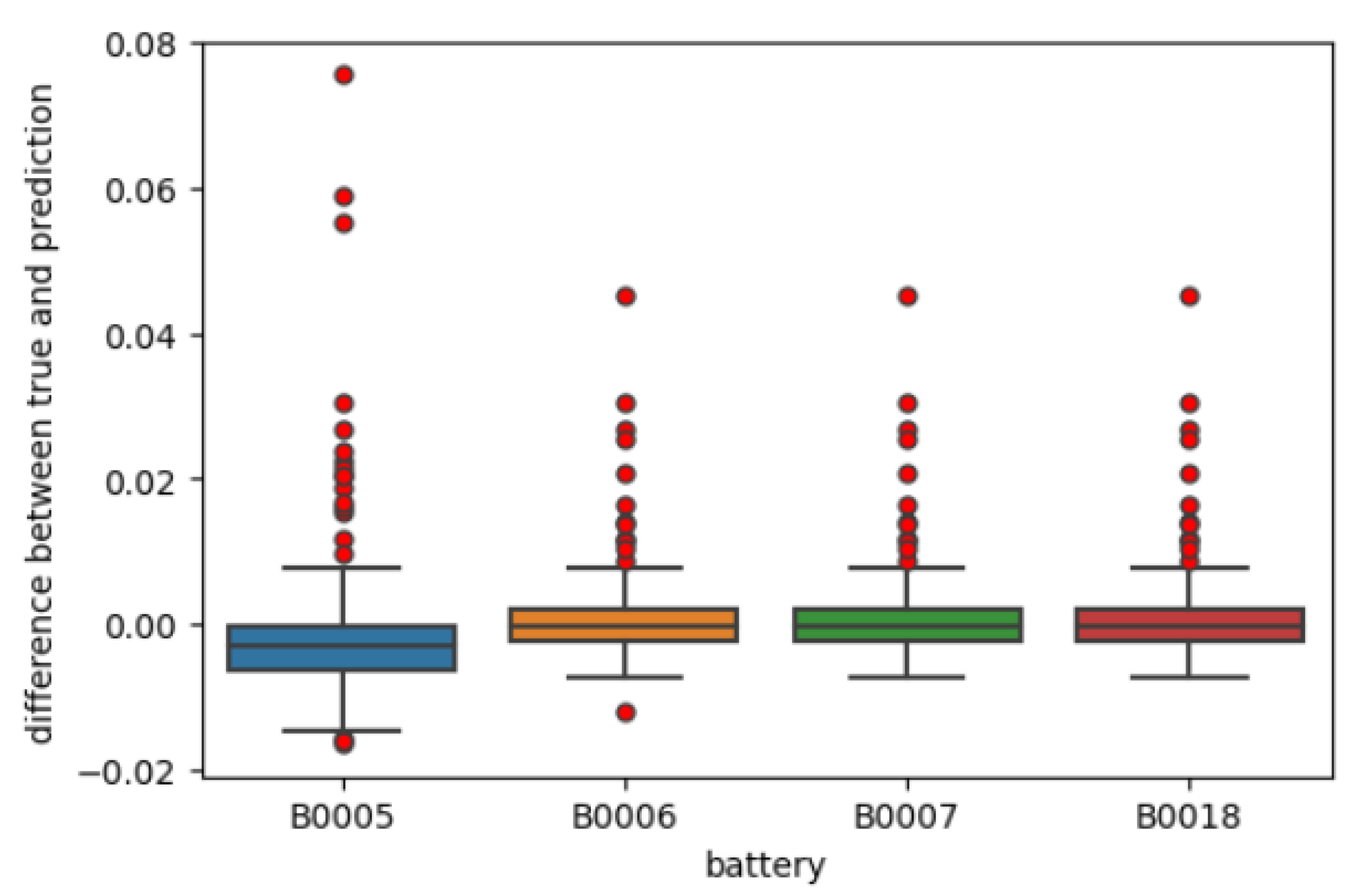
5.1. Comparative Analysis and Evaluation
5.2. Encoder Optimisation and Effects
5.3. Model Comparison Using the Diebold-Mariano Test
6. Conclusions
Author Contributions
Funding
Institutional Review Board Statement
Informed Consent Statement
Data Availability Statement
Conflicts of Interest
References
- Armand, M.; Tarascon, J. Building Better Batteries. Nature 2008, 451, 652–657. [Google Scholar] [CrossRef] [PubMed]
- Severson, K.; Attia, P.; Jin, N.; Perkins, N.; Jiang, B.; Yang, Z.; Chen, M.; Aykol, M.; Herring, P.; Fraggedakis, D.; et al. Data-Driven Prediction of Battery Cycle Life Before Capacity Degradation. Nat. Energy 2019, 4, 383–391. [Google Scholar] [CrossRef]
- Singh, B.; Dubey, P.K. Distributed power generation planning for distribution networks using electric vehicles: Systematic attention to challenges and opportunities. J. Energy Storage 2022, 48, 104030. [Google Scholar] [CrossRef]
- Tran, M.K.; Panchal, S.; Khang, T.D.; Panchal, K.; Fraser, R.; Fowler, M. Concept Review of a Cloud-Based Smart Battery Management System for Lithium-Ion Batteries: Feasibility, Logistics, and Functionality. Batteries 2022, 8, 19. [Google Scholar] [CrossRef] [PubMed]
- Zheng, Z.; Peng, J.; Deng, K.; Gao, K.; Li, H.; Chen, B.; Yang, Y.; Huang, Z. A Novel Method for Lithium-Ion Battery Remaining Useful Life Prediction Using Time Window and Gradient Boosting Decision Trees. In Proceedings of the 2019 10th International Conference on Power Electronics and ECCE Asia (ICPE 2019-ECCE Asia), Busan, Republic of Korea, 27–30 May 2019; pp. 3297–3302. [Google Scholar]
- Chen, Z.; Sun, M.; Shu, X.; Shen, J.; Xiao, R. On-board state of health estimation for lithium-ion batteries based on random forest. In Proceedings of the 2018 IEEE International Conference on Industrial Technology (ICIT), Lyon, France, 20–22 February 2018; pp. 1754–1759. [Google Scholar]
- Sun, F.; Liu, J.; Wu, J.; Pei, C.; Lin, X.; Ou, W.; Jiang, P. BERT4Rec: Sequential recommendation with bidirectional encoder representations from transformer. In Proceedings of the 28th ACM International Conference on Information and Knowledge Management, Beijing, China, 3–7 November 2019; pp. 1441–1450. [Google Scholar]
- Ma, M.; Mao, Z. Deep-Convolution-Based LSTM Network for Remaining Useful Life Prediction. IEEE Trans. Ind. Inform. 2021, 17, 1658–1667. [Google Scholar] [CrossRef]
- Khalid, A.; Sundararajan, A.; Acharya, I.; Sarwat, A.I. Prediction of Li-Ion Battery State of Charge Using Multilayer Perceptron and Long Short-Term Memory Models. In Proceedings of the 2019 IEEE Transportation Electrification Conference and Expo (ITEC), Detroit, MI, USA, 19–21 June 2019; pp. 1–6. [Google Scholar]
- Shi, Z.; Chehade, A. A dual-LSTM framework combining change point detection and remaining useful life prediction. Reliab. Eng. Syst. Saf. 2021, 205, 107257. [Google Scholar] [CrossRef]
- Chen, D.; Hong, W.; Zhou, X. Transformer Network for Remaining Useful Life Prediction of Lithium-Ion Batteries. IEEE Access 2022, 10, 19621–19628. [Google Scholar] [CrossRef]
- Hu, W.; Zhao, S. Remaining useful life prediction of lithium-ion batteries based on wavelet denoising and transformer neural network. Front. Energy Res. 2022, 10, 969168. [Google Scholar] [CrossRef]
- Barre, A.; Deguilhem, B.; Grolleau, S.; Gerard, M.; Suard, F.; Riu, D. A Review on Lithium-Ion Battery Ageing Mechanisms and Estimations for Automotive Applications. J. Power Sources 2013, 241, 680–689. [Google Scholar] [CrossRef]
- Xing, Y.; Ma, W.; Tsui, K.L.; Pecht, M. An ensemble model for predicting the remaining useful performance of lithium-ion batteries. Microelectron. Reliab. 2011, 51, 1084–1091. [Google Scholar] [CrossRef]
- Hlal, M.I.; Ramachandaramurthy, V.K.; Sarhan, A.; Pouryekta, A.; Subramaniam, U. Optimum battery depth of discharge for off-grid solar PV/battery system. J. Energy Storage 2019, 26, 100999. [Google Scholar] [CrossRef]
- Wang, J.; Liu, P.; Hicks-Garner, J.; Sherman, E.; Soukiazian, S.; Verbrugge, M.; Tataria, H.; Musser, J.; Finamore, P. Cycle-life model for graphite-LiFePO4 cells. J. Power Sources 2011, 196, 3942–3948. [Google Scholar] [CrossRef]
- Kwon, S.; Han, D.; Park, J.; Lee, P.Y.; Kim, J. Joint state-of-health and remaining-useful-life prediction based on multi-level long short-term memory model prognostic framework considering cell voltage inconsistency reflected health indicators. J. Energy Storage 2022, 55, 105731. [Google Scholar] [CrossRef]
- Hesse, H.C.; Schimpe, M.; Kucevic, D.; Jossen, A. Lithium-Ion Battery Storage for the Grid—A Review of Stationary Battery Storage System Design Tailored for Applications in Modern Power Grids. Energies 2017, 10, 2107. [Google Scholar] [CrossRef]
- Karoń, G. Energy in Smart Urban Transportation with Systemic Use of Electric Vehicles. Energies 2022, 15, 5751. [Google Scholar] [CrossRef]
- Cakiroglu, C.; Islam, K.; Bekdaş, G.; Nehdi, M.L. Data-driven ensemble learning approach for optimal design of cantilever soldier pile retaining walls. Structures 2023, 51, 1268–1280. [Google Scholar] [CrossRef]
- Zhang, S.Y.; Chen, S.Z.; Jiang, X.; Han, W.S. Data-driven prediction of FRP strengthened reinforced concrete beam capacity based on interpretable ensemble learning algorithms. Structures 2022, 43, 860–877. [Google Scholar] [CrossRef]
- Guo, W.; Sun, Z.; Vilsen, S.B.; Meng, J.; Stroe, D.I. Review of “grey box” lifetime modeling for lithium-ion battery: Combining physics and data-driven methods. J. Energy Storage 2022, 56 Pt A, 105992. [Google Scholar] [CrossRef]
- Xu, L.; Deng, Z.; Xie, Y.; Lin, X.; Hu, X. A novel hybrid physics-based and data-driven approach for degradation trajectory prediction in Li-ion batteries. IEEE Trans. Transp. Electrif. 2022, 9, 2628–2644. [Google Scholar] [CrossRef]
- Chen, L.; Tong, Y.; Dong, Z. Li-ion battery performance degradation modeling for the optimal design and energy management of electrified propulsion systems. Energies 2020, 13, 1629. [Google Scholar] [CrossRef]
- Li, Y.; Zhou, Z.; Wu, W.T. Three-dimensional thermal modeling of Li-ion battery cell and 50 V Li-ion battery pack cooled by mini-channel cold plate. Appl. Therm. Eng. 2019, 147, 829–840. [Google Scholar] [CrossRef]
- Tran, M.K.; DaCosta, A.; Mevawalla, A.; Panchal, S.; Fowler, M. Comparative Study of Equivalent Circuit Models Performance in Four Common Lithium-Ion Batteries: LFP, NMC, LMO, NCA. Batteries 2021, 7, 51. [Google Scholar] [CrossRef]
- Varini, M.; Campana, P.E.; Lindbergh, G. A semi-empirical, electrochemistry-based model for Li-ion battery performance prediction over lifetime. J. Energy Storage 2019, 25, 100819. [Google Scholar] [CrossRef]
- Saha, B.; Goebel, K.; Poll, S.; Christophersen, J. Prognostics Methods for Battery Health Monitoring Using a Bayesian Framework. IEEE Trans. Instrum. Meas. 2007, 58, 291–296. [Google Scholar] [CrossRef]
- Burgos-Mellado, C.; Orchard, M.E.; Kazerani, M.; Cárdenas, R.; Sáez, D. Particle-filtering-based estimation of maximum available power state in Lithium-Ion batteries. Appl. Energy 2016, 161, 349–363. [Google Scholar] [CrossRef]
- Berecibar, M.; Gandiaga, I.; Villarreal, I.; Omar, N.; Van Mierlo, J.; Van den Bossche, P. Critical Review of State of Health Estimation Methods of Li-Ion Batteries for Real Applications. Renew. Sustain. Energy Rev. 2016, 56, 572–587. [Google Scholar] [CrossRef]
- Nhu, V.H.; Shahabi, H.; Nohani, E.; Shirzadi, A.; Al-Ansari, N.; Bahrami, S.; Miraki, S.; Geertsema, M.; Nguyen, H. Daily Water Level Prediction of Zrebar Lake (Iran): A Comparison between M5P, Random Forest, Random Tree and Reduced Error Pruning Trees Algorithms. ISPRS Int. J. Geo-Inf. 2020, 9, 479. [Google Scholar] [CrossRef]
- Cha, G.W.; Moon, H.; Kim, Y.m.; Hong, W.; Hwang, J.H.; Park, W.; Kim, Y.C. Development of a Prediction Model for Demolition Waste Generation Using a Random Forest Algorithm Based on Small DataSets. Int. J. Environ. Res. Public Health 2020, 17, 6997. [Google Scholar] [CrossRef]
- Nascimento, R.G.; Corbetta, M.; Kulkarni, C.S.; Viana, F.A. Hybrid physics-informed neural networks for lithium-ion battery modeling and prognosis. J. Power Sources 2021, 513, 230526. [Google Scholar] [CrossRef]
- Ardeshiri, R.R.; Razavi-Far, R.; Li, T.; Wang, X.; Ma, C.; Liu, M. Gated recurrent unit least-squares generative adversarial network for battery cycle life prediction. Measurement 2022, 196, 111046. [Google Scholar] [CrossRef]
- Yang, Y.; Wu, Z.; Yang, Y.; Lian, S.; Guo, F.; Wang, Z. A Survey of Information Extraction Based on Deep Learning. Appl. Sci. 2022, 12, 9691. [Google Scholar] [CrossRef]
- Yin, A.; Tan, Z.; Tan, J. Life Prediction of Battery Using a Neural Gaussian Process with Early Discharge Characteristics. Sensors 2021, 21, 1087. [Google Scholar] [CrossRef] [PubMed]
- Zhao, J.; Ling, H.; Liu, J.; Wang, J.; Burke, A.F.; Lian, Y. Machine learning for predicting battery capacity for electric vehicles. eTransportation 2023, 15, 100214. [Google Scholar] [CrossRef]
- Vaswani, A.; Shazeer, N.; Parmar, N.; Uszkoreit, J.; Jones, L.; Gomez, A.N.; Kaiser, L.u.; Polosukhin, I. Attention is All you Need. In Advances in Neural Information Processing Systems; Guyon, I., Luxburg, U.V., Bengio, S., Wallach, H., Fergus, R., Vishwanathan, S., Garnett, R., Eds.; Curran Associates, Inc.: Red Hook, NY, USA, 2017; Volume 30. [Google Scholar]
- Wu, L.; Li, S.; Hsieh, C.J.; Sharpnack, J. SSE-PT: Sequential Recommendation Via Personalized Transformer. In Proceedings of the 14th ACM Conference on Recommender Systems, Association for Computing Machinery, New York, NY, USA, 18–22 September 2020; pp. 328–337. [Google Scholar]
- Cornia, M.; Stefanini, M.; Baraldi, L.; Cucchiara, R. Meshed-Memory Transformer for Image Captioning. In Proceedings of the IEEE/CVF Conference on Computer Vision and Pattern Recognition (CVPR), Seattle, WA, USA, 13–19 June 2020. [Google Scholar]
- Gu, F. Research on Residual Learning of Deep CNN for Image Denoising. In Proceedings of the 2022 7th International Conference on Intelligent Computing and Signal Processing (ICSP), Xi’an, China, 15–17 April 2022; pp. 1458–1461. [Google Scholar]
- Alkesaiberi, A.; Harrou, F.; Sun, Y. Efficient Wind Power Prediction Using Machine Learning Methods: A Comparative Study. Energies 2022, 15, 2327. [Google Scholar] [CrossRef]


| Dataset Models | Sample Size | Learning Rate | Depth | Hidden Size | Trans Reg |
|---|---|---|---|---|---|
| DT | 16 | 0.001 | 2 | 64 | |
| RF | 16 | 0.01 | 2 | 8 | |
| MLP | 16 | 0.01 | 2 | 8 | |
| RNN | 16 | 0.001 | 2 | 64 | |
| LSTM | 16 | 0.001 | 2 | 64 | |
| GRU | 16 | 0.001 | 2 | 64 | |
| Dual-LSTM | 16 | 0.001 | 2 | 64 | |
| DeTransformer | 16 | 0.005 | 1 | 32 | |
| DTNN | 16 | 0.005 | 1 | 32 |
| RF | DT | MLP | RNN | LSTM | GRU | Dual-LSTM | DeTransformer | DTNN | |
|---|---|---|---|---|---|---|---|---|---|
| RE | 0.2969 | 0.3997 | 0.3871 | 0.2924 | 0.2716 | 0.3342 | 0.2641 | 0.2312 | 0.0351 |
| RMSE | 0.0962 | 0.1522 | 0.1402 | 0.0827 | 0.0952 | 0.0916 | 0.0831 | 0.0792 | 0.005 |
| MAE | 0.0838 | 0.163 | 0.1564 | 0.0744 | 0.0866 | 0.0912 | 0.0883 | 0.0852 | 0.0272 |
| 0.977 | 0.971 | 0.972 | 0.965 | 0.968 | 0.967 | 0.969 | 0.975 | 0.991 | |
| MAPE | 1.431 | 1.672 | 1.215 | 1.542 | 1.479 | 1.452 | 1.353 | 1.120 | 0.632 |
| 26.1 | 35.3 | 34.6 | 25.6 | 23.8 | 27.4 | 23 | 20.8 | 3.2 |
| Method | p-Value | DM Value |
|---|---|---|
| RF | 0.019 | −4.17 |
| DT | 0.015 | −5.26 |
| MLP | 0.018 | −4.35 |
| RNNs | 0.024 | −4.12 |
| LSTM | 0.026 | −3.24 |
| GRU | 0.031 | −4.01 |
| Dual-LSTM | 0.024 | −2.95 |
| DeTransformer | 0.04 | −1.98 |
Disclaimer/Publisher’s Note: The statements, opinions and data contained in all publications are solely those of the individual author(s) and contributor(s) and not of MDPI and/or the editor(s). MDPI and/or the editor(s) disclaim responsibility for any injury to people or property resulting from any ideas, methods, instructions or products referred to in the content. |
© 2023 by the authors. Licensee MDPI, Basel, Switzerland. This article is an open access article distributed under the terms and conditions of the Creative Commons Attribution (CC BY) license (https://creativecommons.org/licenses/by/4.0/).
Share and Cite
Han, Y.; Li, C.; Zheng, L.; Lei, G.; Li, L. Remaining Useful Life Prediction of Lithium-Ion Batteries by Using a Denoising Transformer-Based Neural Network. Energies 2023, 16, 6328. https://doi.org/10.3390/en16176328
Han Y, Li C, Zheng L, Lei G, Li L. Remaining Useful Life Prediction of Lithium-Ion Batteries by Using a Denoising Transformer-Based Neural Network. Energies. 2023; 16(17):6328. https://doi.org/10.3390/en16176328
Chicago/Turabian StyleHan, Yunlong, Conghui Li, Linfeng Zheng, Gang Lei, and Li Li. 2023. "Remaining Useful Life Prediction of Lithium-Ion Batteries by Using a Denoising Transformer-Based Neural Network" Energies 16, no. 17: 6328. https://doi.org/10.3390/en16176328
APA StyleHan, Y., Li, C., Zheng, L., Lei, G., & Li, L. (2023). Remaining Useful Life Prediction of Lithium-Ion Batteries by Using a Denoising Transformer-Based Neural Network. Energies, 16(17), 6328. https://doi.org/10.3390/en16176328