Article

A Power External Transmission Strategy for Regional Power Grids Considering Internal Flexibility Supply and Demand Balance

1
College of Electrical Engineering, Zhejiang University, Hangzhou 310027, China
2
Inner Mongolia Power (Group) Co., Ltd., Hohhot 010020, China
3
Inner Mongolia Electric Power Economic and Technical Research Institute, Hohhot 010020, China
*
Author to whom correspondence should be addressed.
Energies 2023, 16(17), 6323; https://doi.org/10.3390/en16176323
Submission received: 14 June 2023 / Revised: 31 July 2023 / Accepted: 6 August 2023 / Published: 31 August 2023
(This article belongs to the Section F: Electrical Engineering)

Abstract

:
This paper provides an optimization strategy for flexible operation at the system level to guide the real-time flexible ramping of the power grid. Firstly, the concept of regional power grid flexibility is clarified, and the ramping factor is proposed as a flexibility metric. On this basis, taking the output priority of each node as the objective function and considering constraints such as line flow, power balance, and system flexibility, a mathematical model for regional power grid transmitting flexible power externally is proposed. Compared with the traditional models, this model focuses more on flexibility rather than economy. A case analysis based on the improved IEEE 30-Bus System verifies the feasibility and effectiveness of the proposed strategy and its advantages over the traditional models.

1. Introduction

Due to the desire to solve the increasingly serious energy crisis and environmental problems [1], the concept of Carbon Neutrality has gained momentum in recent years [2]. With the proportion of its power generation rising gradually, the renewable energy will become the main resources for electricity generation in the future power system. However, when supply becomes more variable and less certain, as with some renewable sources of electricity like wind and solar PV that fluctuate with the weather [3], power systems are exposed to the challenge of imbalance of production and consumption of electricity. In order to cope with this challenge, the system is required to have the ability to react to a sudden change and accommodate a new status within an acceptable time period and cost [4]. In this background, the International Energy Agency (IEA) released a special report in 2008, putting forward the concept of “flexibility of power system” with an emphasis on increasing the system ability to cope with power fluctuations by enhancing system flexibility [5].
Usually, the power system flexibility is considered to include the node flexibility and the grid transmission flexibility [6]. Node flexibility refers to the power ramping ability of the flexible resources at each node, which are widely distributed in the power system [7]. The node flexibility maintains an in situ balance with the local net load fluctuation; simultaneously, it provides flexibility support and supply to the external system in the unit of a node at the same time, making the node a basic source unit of the power system flexibility [8].
However, the current approaches to node flexibility and grid transmission flexibility only address the allocation of flexible resources within the power grid. They do not tackle the challenge of how regional power grids can transmit (or absorb) flexible power externally. In this regard, researchers have characterized the power transmission ability of regional power grids using various methods. For instance, NERC proposes the network response method and rated path method based on linear distribution factors to analyze the response characteristics of actual networks and determine the transmission capacity of a power system [9]. Another reference [10] maximizes the active transmission power of boundary sections or single connecting lines while considering steady-state and stable operation requirements as constraints. This enables the calculation of power system transmission capacity to be transformed into solving the optimal power flow problem.
In some cases, references [11] use 2m- and 2m+1-point estimation methods to approximate the probability density function of power system transmission capacity. However, this approach requires fitting the continuous uncertainty distribution based on historical data, which may introduce fitting errors into subsequent calculations. To address this issue, reference [12] eliminates the need for distribution fitting. Instead, it directly utilizes the Sparse Polynomial Chaos Expansion Method with the original historical data to obtain multi-order moment information of the power system transmission capacity. Additionally, reference [13] samples wind speeds using the non-sequential Monte Carlo method, calculates power samples of wind turbines based on wind speed power conversion curves, and then determines the power system transmission capacity under each sample. Reference [14] illuminates the transmission power of the power grid by calculating the available transmission capacity using the grid flow method; reference [15] iteratively updates the power feasible region of the interconnection line based on the searched vertices; reference [16] selects variables such as transmission power of interconnection lines as planning parameters to characterize the feasible region of interconnection line power.
While these methods above focus on the transmission lines between regional power grids, they do not fully account for the distribution of internal flexibility when regional power grids exchange power externally. In response to this issue, this paper defines the flexibility of regional power grids and proposes a flexible power transmission strategy based on the ramping factor for regional power grids. This strategy can not only calculate the flexible resources injected at each node in the regional power grid as well as the flexible power transmitting through each line, but also guide the power transmission between different levels of power grids.

2. Concept of Flexibility

Scholars at home and abroad have conducted extensive research on the concept of power system flexibility and formed a preliminary system. This chapter proposes the concept of regional power grid flexibility in this system and provides a clear flexibility metric.

2.1. Definition of Flexibility

Nowadays, the importance of flexibility is fully recognized, but this concept has not yet been clearly defined. IEA believes that flexibility is the ability of the power system to maintain reliability by adjusting generation or load in the face of large disturbances, i.e., the ability to quickly respond to foreseeable and unforeseeable events [3]. The Midcentral Independent System Operator (MISO) defines flexibility as the ability to meet the system’s potential ramping needs by dispatching flexible resources during real-time operation [17]. The North American Electric Reliability Corporation (NERC) defines flexibility as the ability of power system flexible resources to meet the changes of net load, where the net load refers to the total load minus the output of variable sources (wind, photovoltaic, etc.) [18]. The definition of flexibility in academia [19,20,21,22], although slightly different, is basically consistent, i.e., the ability of the power system to respond to power changes.
Essentially, the flexibility of the power system originates from the requirement of real-time balance between power supply and demand, reflecting the system’s ability to maintain the supply–demand balance when the supply–demand relationship changes. Based on the definition of NERC and combining the opinions of many scholars in the academic community [14,15,16,17], this paper proposes the following definition: flexibility is the ability of various components of the power system (power sources, loads, local grids, etc.) or the power system itself to meet changes of net loads and respond to power regulation needs. Among them, flexible resources mainly include generator units with flexible ramping capabilities on the generation side (thermal power units, hydroelectric units, nuclear power units, pumped storage power stations, etc.) and interruptible/ramp-able loads on the load side (air conditionings, water heaters, etc.); and net load refers to the total load minus the output of variable power sources (wind, photovoltaic, etc.).
For power systems with extremely wide coverage, such as State Grid and Southern Power Grid in China, when conducting research on flexibility, it is necessary to consider not only the node flexibility and the grid transmission flexibility, but also the flexibility of a certain sub grid within the power system itself. Therefore, this paper proposes the concept of regional power grid flexibility and defines it as the ability of the entire regional power grid to meet its own real-time balance of power supply and demand, as well as the ability to transmit flexible power externally, where flexible power is the output variation of flexible resources during the flexible ramping process.

2.2. Metric of Flexibility

Before conducting research on flexible ramping, flexibility metric must be clarified. This paper uses the ramping factor as a flexibility metric, and its acquisition method is as follows.

2.2.1. Fluctuation Amplitude of Net Load (FANL)

As mentioned in Section 2.1, net load refers to the total load minus the output of variable power sources such as wind and photovoltaic. For any node i within a ramping period T, the maximum possible increase in the net load (namely “up fluctuation amplitude of net load” at node i) is set as F A N L i U , and the maximum possible decrease (namely “down fluctuation amplitude of net load” at node i) is set as as F A N L i D . Similarly for a power grid within a ramping period T, the up-fluctuation amplitude of net load of that grid is set up as F A N L U , and the down-fluctuation amplitude of net load is set as F A N L D .
F A N L i U and F A N L i D can be obtained by the following method: First, the load and output forecasting methods are used to obtain node i’s net load sequence at time scale T, which is { P i net ( n T ) | n N } . Second, the first-order difference operation is used on the net load sequence to yield the net load fluctuation power sequence, which is { P i , n net | P i net = P i net ( ( n + 1 ) T ) P i net ( n T ) , n N } . Third, the maximum value of this sequence is found to obtain the FANL:
{ F A N L i U = max { P i , n net | P i net = P i net ( ( n + 1 ) T ) P i net ( n T ) , n N } F A N L i D = min { P i , n net | P i net = P i net ( ( n + 1 ) T ) P i net ( n T ) , n N } .
Similarly, F A N L U and F A N L D can also be obtained from the following equation:
{ F A N L U = max { P i , n net | P i net = P i net ( ( n + 1 ) T ) P i net ( n T ) , n N } F A N L D = min { P i , n net | P i net = P i net ( ( n + 1 ) T ) P i net ( n T ) , n N } .

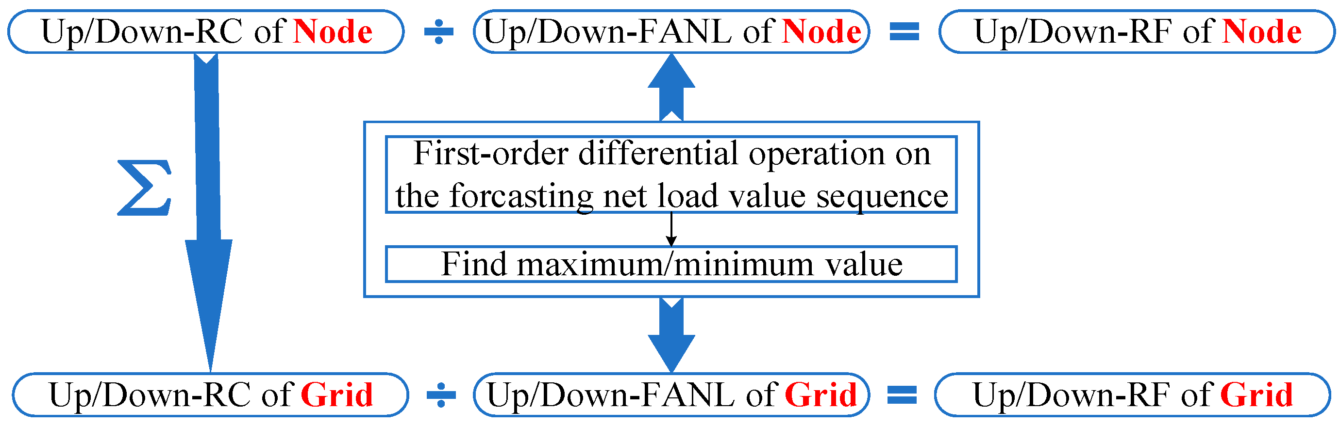
2.2.2. Ramping Capability (RC)

When the net load fluctuates, the output of flexible resources at node i ramps to maintain the system power stability according to changes in power supply and demand. The maximum power that can be ramped upwards at node i during the period T (namely “up ramping capability” at node i) os R C i U , and the maximum power that can be ramped downwards (namely “down ramping capability” at node i) is R C i D . It is clear that RC is the sum of the differences between the maximum (or minimum) output and normal output of each flexible resource. Then, R C i U and R C i D can be obtained by the following equation:
{ R C i U = k ( P i k , g , max P i k , g ) R C i D = k ( P i k , g P i k , g , min ) ,
where Pik,g is the output power of the kth flexible resource at node i before flexible ramping; Pik,g,min and Pik,g,max are, respectively, the upper and lower limits of the flexible resource output power.
Similarly, as for a power grid, the up-ramping capacity of the grid during the period T is R C U , and the down-ramping capacity is R C D ; then, R C U and R C D can be obtained by the following equation:
{ R C U = i k ( P i k , g , max P i k , g ) R C D = i k ( P i k , g P i k , g , min ) .
From the above definition, it can be seen that real-time flexible ramping of the power grid is the process of consuming RC. After a one-time ramping, some nodes still have a certain amount of RC, which we call the “remaining ramping capability”. Similar to Equation (4), the remaining RC of the entire grid is the sum of that of each node.

2.2.3. Ramping Factor (RF)

Based on the above definitions, this paper defines the ratio of RC to FANL as the “Ramping Factor” (RF). The RF of node i is
{ R F i U = R C i U F A N L i U R F i D = R C i D F A N L i D ,
where R F i U is the “up-ramping factor of node i” and R F i D is the “down-ramping factor of node i”.
In a power system, conventional nodes may be connected to power sources or loads. If the subordinate grid is equivalent to a power source or a load, then the entire subordinate grid can also be considered as one node, and we call this node a “generalized node”. It is not difficult to see that as the research subject, the local grid can also be regarded as a generalized node of the superior grid. We define the ramping factor of this generalized node in the superior grid as the “ramping factor of grid”, and the ramping factor of the local grid is
{ R F U = R C U F A N L U R F D = R C D F A N L D ,
where R F U is the “up-ramping factor of grid” and R F D is the “down-ramping factor of grid”.
The ramping factor is the flexibility metric. Obviously, the larger the ramping factor, the more abundant the flexibility of the node or system. For ease of understanding, Figure 1 shows the relationship among FANL, RC, and RF.

3. Power Transmission Strategy for Regional Power Grids

The previous chapter provided the flexibility metric of a power grid, namely the ramping factor. Based on this metric, this chapter proposes a specific mathematical model to guide the flexible ramping of the power grid itself and its transmitting externally flexible power.

3.1. Objective Function

During system operation, if there is a shortage of power supply from the superior grid requiring the local grid to transmit externally the additional power of ΔP (namely the flexible power mentioned in Section 2.1) within time T, then it is necessary to develop a transmission strategy for flexible power based on the RF. We take the case of up-ramping as an example, i.e., set the ΔP greater than 0.
First of all, we number all nodes according to the up RF from small to large, i.e., node i satisfies R F i R F i + 1 , and the set of all nodes is { 1 , 2 , 3 , M 1 , M } ; there is no concept of RF in the connection node between the local grid and the superior grid, and thus its serial number is set to M + 1. According to the analysis in the previous chapter, the larger the RF, the more flexible the node. Therefore, we determine the priority of flexible resource participation in up-ramping for each node as follows: node M has the highest priority in up-ramping, and if the flexible power provided externally by the local grid is insufficient ΔP, then node M − 1 continues to participate in the up-ramping, and so on. As for the ramping priority of various flexible resources, we offer the highest priority to the energy storage systems, then thermal power units, and finally other types of generators, etc.
In order to ensure that nodes with large up-RFs inject as much flexible power as possible, we should minimize the total number of nodes participating in flexible ramping. We let nodes from number m to number M participate in flexible ramping, i.e., the set of ramping nodes is D = { m , m + 1 , M 1 , M } , so the objective function can be set as
min ( M m + 1 ) .

3.2. Constraint Conditions

Unlike traditional constraints that focus on flexible resources, the constraints in this section focus on nodes. From the definition of RF in the previous chapter, it can be seen that node RC must be obtained before calculating node RF, and the process of calculating node RC (Equations (8) and (9)) already includes constraints on the output power of flexibility resources. Therefore, the constraint conditions in this section no longer consider the node power constraints such as generators, ramp-able loads, energy storages, etc.
Numbered lists can be added as follows:
  • Line flow constraints. According to the principle of power system secure dispatching, after flexible ramping at each node, the power flow of each line (namely the power flowing through the line, in order to distinguish it from the node power P; this paper uses F to represent the power flow) should be kept in the limited range. The mathematical expression for this constraint is
    | F j | F j , max , j = 1 , 2 , ,
    where Fj is the power flowing through line j, which can be calculated from power flow calculations, and Fj,max is the rated transmission capacity of line j. Because this paper focuses on the transmission of active power, Fj can also be calculated from the DC power flow model. We let matrix T be the power transmission distribution factor (PTDF) in the DC power flow model, and its calculation method is shown in Appendix A. Then,
    F j = i T j i ( P i + Δ P i ) ,
    where Tji is the element in the jth row and the ith column of matrix T, namely node i’s distribution factor on line j; Pi is the injection power at node i before the flexible ramping, ΔPi is the additional power generated at node i during the flexible ramping.
  • Power balance constraints. The total demand for flexibility should be equal to the total supply of it, i.e., the flexible power supplied by the local grid ΔP is equal to the sum of the increased injection power at each node, i.e.,
    i Δ P i = Δ P .
  • Flexibility constraints. The increased injection power at each node should not exceed the range allowed by ramping capacity, i.e.,
    R F i D F A N L i D Δ P i R F i U F A N L i U .
  • Other constraints. The nodes involved in flexible ramping should be elements of the set D, i.e.,
i { m , m + 1 , M 1 , M } .

3.3. Mathematical Model

In summary, the mathematical model for regional power grid supplying flexible power externally is
arg min f ( m ) = M m + 1 s . t . { | i T j i ( P i + Δ P i ) | F j , max i Δ P i = Δ P R F i D F A N L i D Δ P i R F i U F A N L i U i { m , m + 1 , M 1 , M } ,
where ΔPi is the quantity to be solved, and the remaining quantities are known.
If ΔP is less than 0, it means that the superior grid requires additional power consumption from the local power grid, and the injection power at each node needs to be decreased, which is the case of down-ramping. At this point, it is only necessary to renumber all nodes from small to large according to the down-RF, and the rest of the derivation process is the same as in the case of up-ramping. Then, the mathematical model for regional power grid absorbing externally flexible power can be obtained, which is just the same as in Equation (13).
It is worth noting that the mathematical model proposed in this paper places flexibility first, while traditional mathematical models only focus on economic benefits, which may lead to a lack of ramping capability in the solution results. We verify this in the next chapter.

4. Case Analysis of Flexible Operation

In this section, the IEEE 30-Bus System [23] is taken as an example to study the specific application of RF. The circuit diagram of this system is shown in Figure 2.

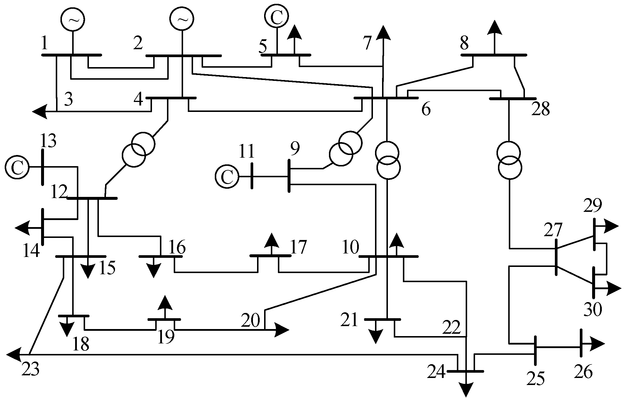
4.1. Improved IEEE 30-Bus System

The classic IEEE 30-Bus System has two voltage levels, 132 kV and 33 kV, respectively. This system provides upper and lower limits of power output data for each generator and fixed load data for each node, but does not include power fluctuation data for each node in the strategy proposed in Chapter 3. Therefore, we made some improvements to this system. According to the theory in Section 2.2.3, we treat the 132 kV part of the classical system as the local grid and the 33 kV part as the subordinate grid. The topology of the improved system is shown in Figure 3a. The node data and branch data of the improved system are the same as those of the classic system, as shown in Appendix B.
The differences between the improved system and the classical system include three main aspects:
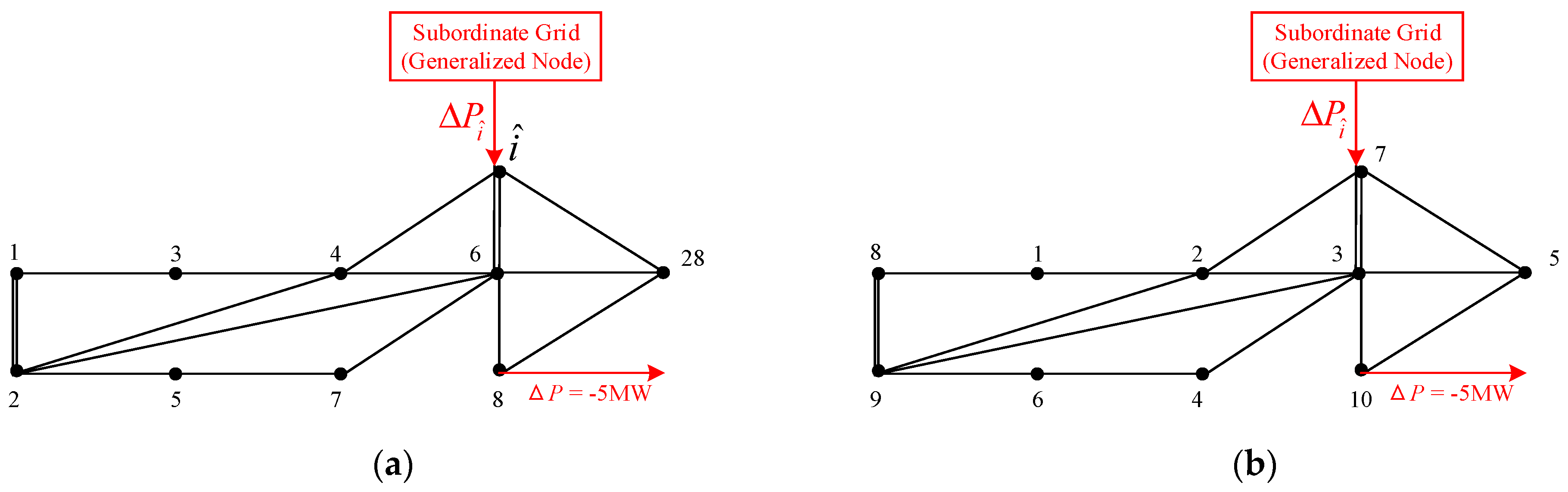
  • In the classic system, there are three connecting lines between the 33 kV part and the 132 kV part; and in the improved system, these three lines are regarded as equipotential points, and the transformer parameters are all converted to the high-voltage side. Therefore, the impedances of the blue line in Figure 3a are all zero.
  • In the improved system, we treat Node 8 as a connection node. From Table A1, we know that the power on the bus of Node 8 reaches the maximum output during normal operation, so the difference between the output and load at Node 8 (5 MW) can be equated to the fixed power delivered from the local grid to the superior grid.
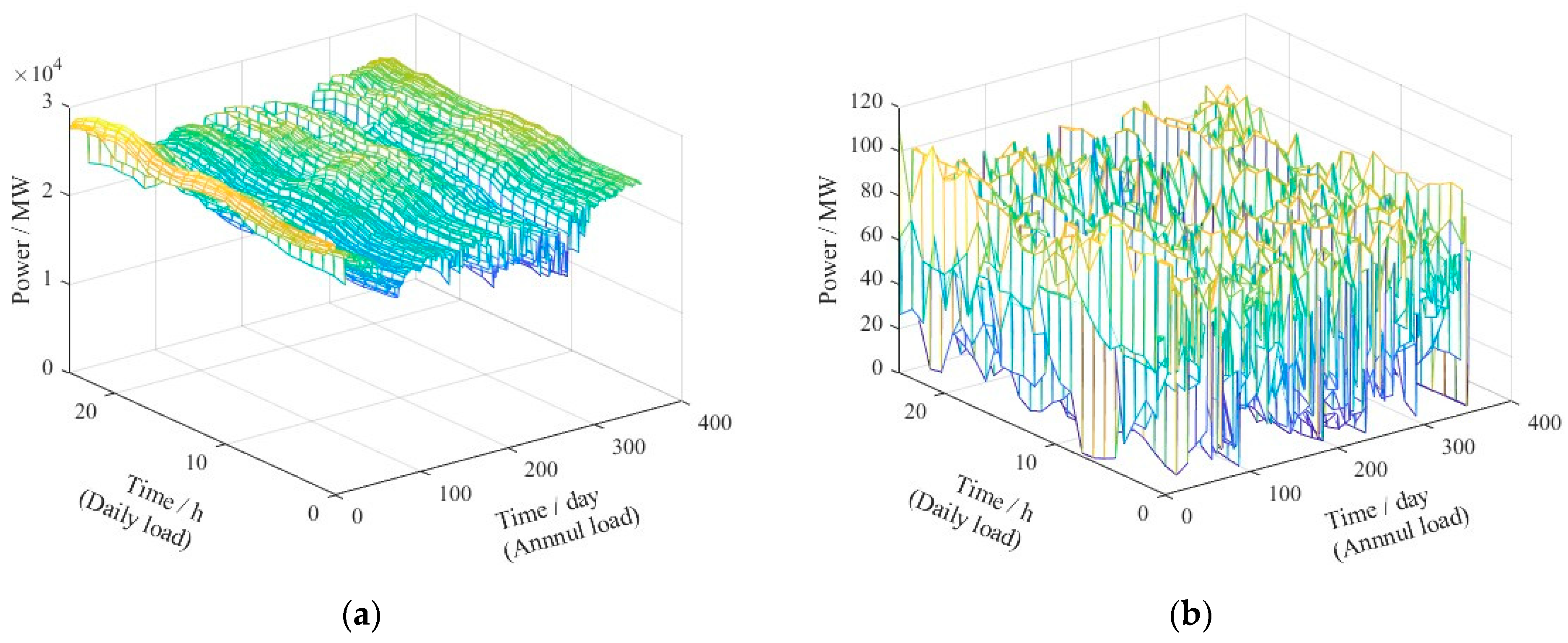
  • In the improved system, both the power and the load show a certain degree of fluctuation and possess a certain degree of ramping capability. The RF and FANL of each node in the local grid are shown in Table 1. According to the characteristics of various flexible resources, the power sources can up-ramp as well as down-ramp the flexible power, while the load can only down-ramp. Therefore, the up-RFs of the nodes with loads but no power sources are zero, and both the up-RFs and down-RFs of the nodes without power sources or loads are zero.
The data in Table 1 are borrowed from the load fluctuation of a provincial power grid in Northwest China. In this grid, there are more than 200 nodes of 220 kV and above voltage levels. The annual load curve of this grid is shown in Figure 4a, and the annual output curve of a typical wind farm in this province is shown in Figure 4b. After first-order differential calculations performed on the annual load of the whole grid and the annual output of the wind farm, we can find out, by employing (4), that the up-FANL of the total load of the grid is 160.97 MW and the down-FANL is 265.24 MW; the up-FANL of the wind farm is 6.62 MW and the down-FANL is 7.34 MW. According to these data, it can be inferred that the FANL of a single 220 kV node of the power grid is in the range of 0~20 kW, and the data in Table 1 is set on this basis.

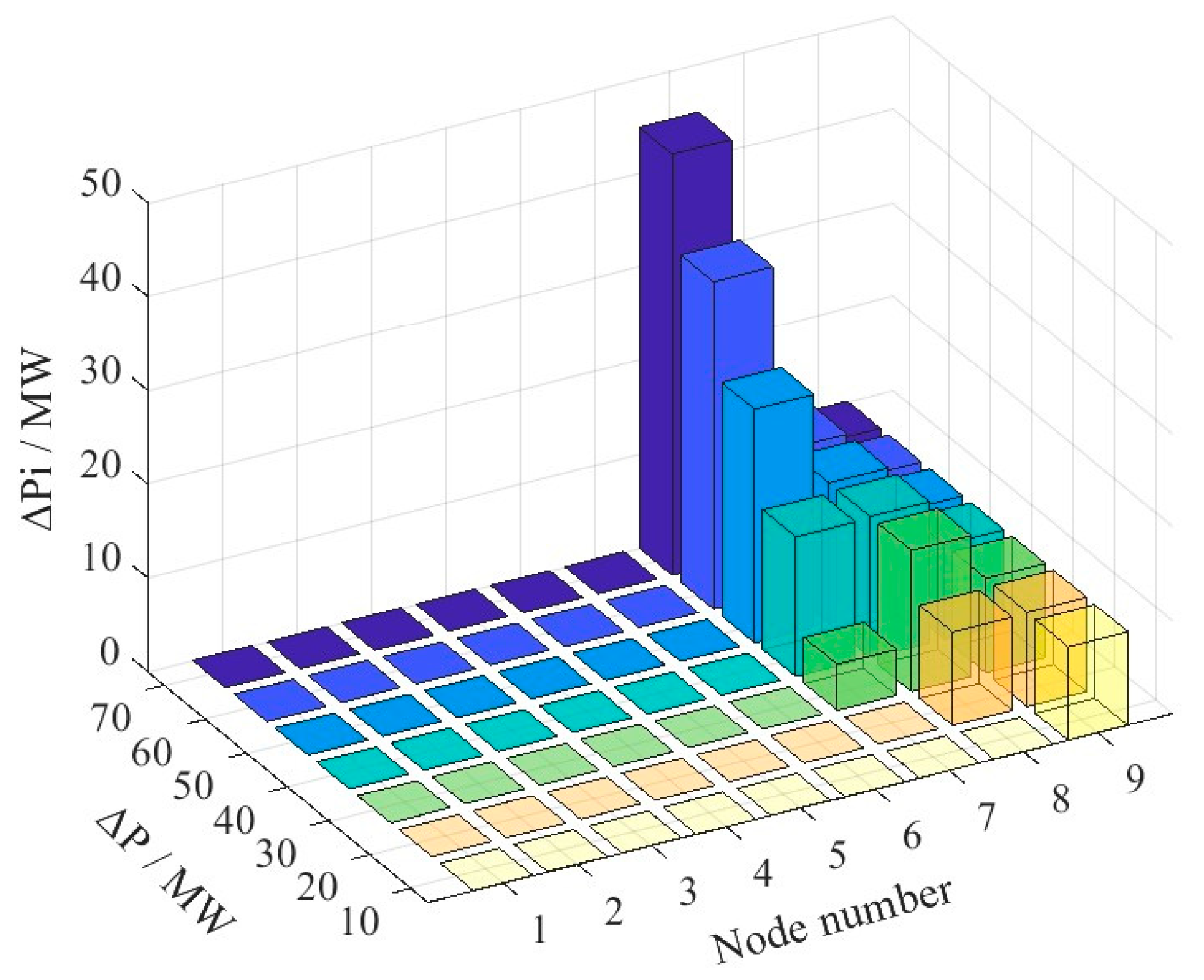
4.2. Flexible Power Distribution of the Local Power Grid

This subsection solves the mathematical model for regional power grid transmitting externally flexible power proposed in Section 3 based on the above-improved IEEE 30-Bus System. During operation, the superior grid requires the improved IEEE 30-Bus System to increase ΔPP > 0) of flexible power supplied externally through Node 8 within 5 min; at this point, a dispatching plan for flexible resources must be developed based on the up RF, and the specific process is described further.
Firstly, each node is renumbered from small to large according to the up RF in Table 1 (connection node is listed at the bottom). The new sequence number is shown in Table 2 and the topology diagram after renumbering is shown in Figure 3b.
Then, each parameter is determined in the mathematical model for regional power grid supplying flexible power externally. The calculation process of the PTDF matrix is shown in Appendix A. The data from Table 1, Table 2, Table A1 and Table A2, as well as the elements in the PTDF matrix, are all substituted into Equation (13) to obtain the mathematical model to be solved in this case, which we call Model 1.
Finally, Model 1 is solved based on the MATLAB 2022b software platform. We set the values of ΔP to 10 MW, 20 MW, 30 MW, 40 MW, 50 MW, 60 MW, and 70 MW, respectively, and we can obtain the additional power generated at each node as shown in Figure 5.
From Figure 5, it can be seen that when the power shortage is 10 W; only Node 9 can participate in flexible ramping to meet the flexibility requirement; when the power shortage is 20 MW, the participation of Nodes 8 and 9 in flexible ramping can meet the flexibility requirements; and when the power shortage is equal to or greater than 30 MW, Nodes 7, 8, and 9 must participate in flexible ramping simultaneously to meet the flexibility requirements.

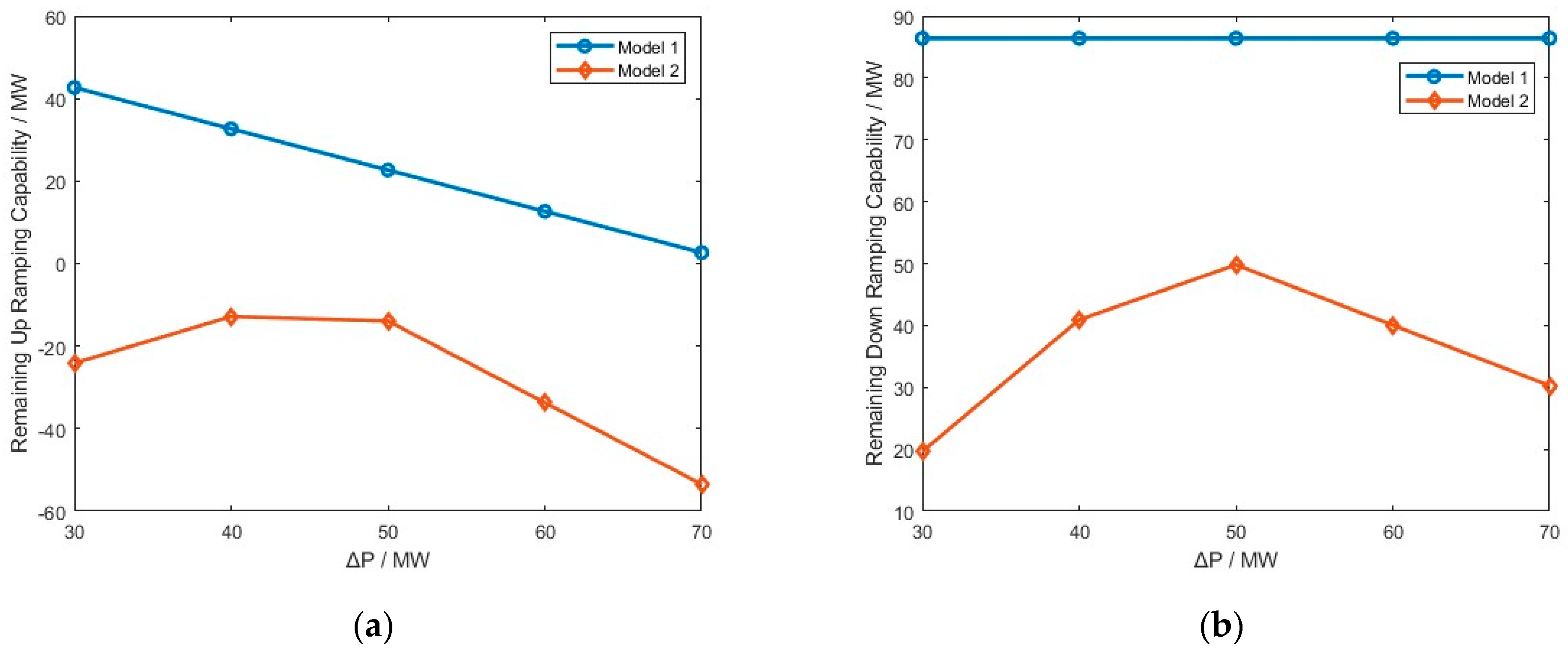
4.3. Comparation with Traditional Method

Traditional mathematical models usually take economy as the objective function when guiding system flexible ramping, while the mathematical model proposed in this paper takes flexibility as the objective function. This section compares the advantages and disadvantages of these two mathematical models.
Similar to the previous section, after completing node renumbering and parameter calculation, we obtain a traditional mathematical model that considers flexibility constraints, which is
arg min f ( Δ P i ) = j R j | i T j i ( P i + Δ P i ) | 2 s . t . { | i T j i ( P i + Δ P i ) | F j , max i Δ P i = Δ P .
Equation (14) is called Model 2. Based on MATLAB, the additional power generated at each node when ΔP takes different values is obtained as shown in Figure 6.
In Figure 6, some nodes exhibit negative additional power generation, which means that when the superior grid requires the local grid to increase external transmission power, in order to reduce local power losses, some nodes experience a decrease in injection power instead of the expected increase. This inevitably results in a considerable waste of flexible power.
According to the definition of the remaining RC in Section 2.2, the remaining ramping capability of the entire grid in this chapter can be obtained by the following equation:
{ R R C U = i ( R F i U F A N L i U Δ P i ) , Δ P i > 0 R R C D = i ( R F i D F A N L i D + Δ P i ) , Δ P i < 0 ,
where RRCU and RRCD are the remaining up-RC and the remaining down-RC of the local grid.
Substituting the data from Figure 5 and Figure 6 into Equation (15), the remaining RC under different operating conditions can be calculated, as shown in Figure 7.
In the actual flexible ramping process, both the remaining up-RC and remaining down-RC can only be greater than or equal to zero, i.e., the dispatching schemes with the remaining RC of less than zero in the calculation results are actually not feasible. From Figure 7, it can be seen that the calculation results of Model 1 can meet the requirement of remaining RC greater than zero under any operating condition, i.e., this model is applicable to all flexibility demands mentioned in this chapter. When ΔP = 30 MW, the remaining up-RC in the calculation results of Model 2 is less than zero, so the mathematical model cannot find a feasible flexible power transmission scheme.
Furthermore, no matter what value ΔP takes, the curve corresponding to Model 1 is always no lower than Model 2, which means that regardless of how much power the superior grid requires the local grid to transmit externally, the operation scheme calculated using Model 1 can always save as much flexible power as possible for the local grid in order to cope with the next flexible ramping.

5. Conclusions

This paper proposes the concept of regional power grid flexibility and its evaluation index RF, and based on this, proposes a flexible power transmission strategy for regional power grids to guide the flexible operation of power systems. The main conclusions are as follows:
  • Regional power grid flexibility means the ability of the entire regional power grid to meet the real-time balance of its own power supply and demand, as well as the ability to transmit flexible power externally, where the flexible power means the change in flexible resource output power during the flexible ramping process. The ramping factor can evaluate both the flexibility of each node and that of the entire regional power grid.
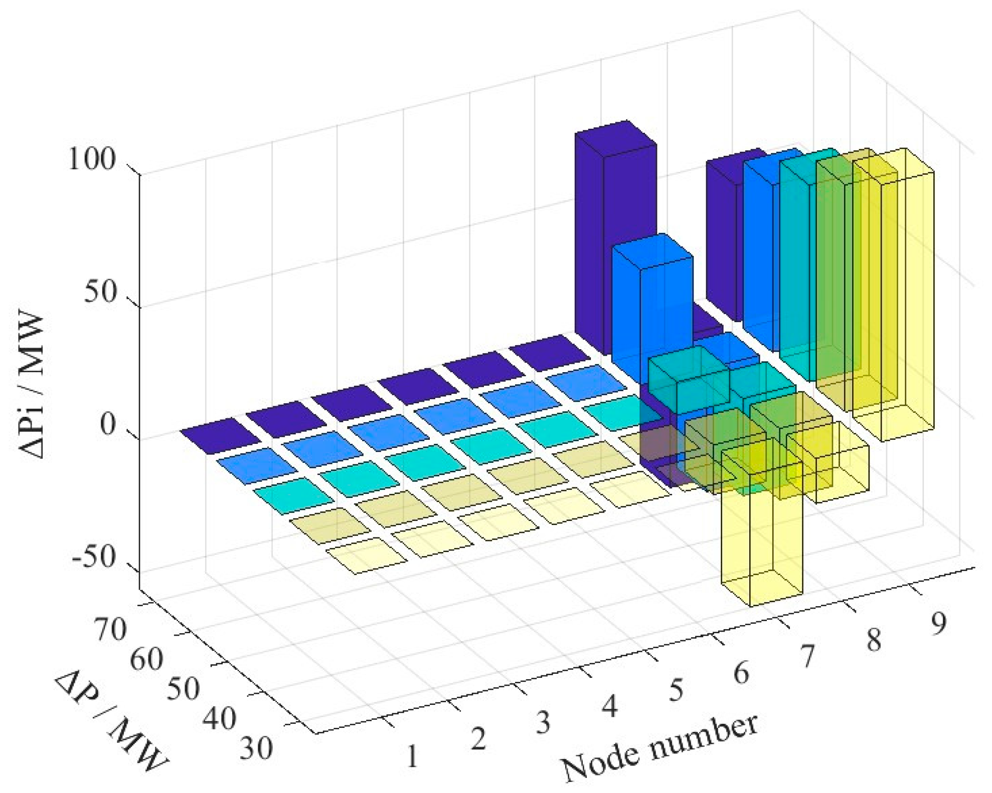
  • The proposed power external transmission strategy can coordinate the flexible resource output at various internal nodes and the flexible power transmission at various internal lines when the local grid exchanges flexibility externally. When transmitting flexible power externally, nodes with a large ramping factor are given priority to participate in flexible ramping, ensuring sufficient residual ramping capability of the regional power grid. In the improved IEEE 30-Bus case study, as the power shortage in the regional power grid gradually increases from 10 MW to 30 MW, Nodes 9, 8, and 7 with larger ramping factors participate in flexible ramping sequentially.
  • The traditional mathematical models only focus on economic benefits, which may lead to a lack of ramping capability in the solution results. Compared with the traditional model, the proposed mathematical model can save as much flexible power as possible for the local grid in order to cope with the next flexible ramping. In the improved IEEE 30-Bus case study, when the power shortage reaches 30 MW, the traditional model fails to find a feasible flexible power transmission scheme. However, the computational results of the proposed model can satisfy the requirement of having the remaining ramping capability greater than zero under any operating condition.

Author Contributions

Conceptualization, Y.Z.; methodology, S.H.; investigation, X.G.; data curation, Z.Z.; writing—review and editing, L.C.; supervision, W.C.; project administration, J.Y. All authors have read and agreed to the published version of the manuscript.

Funding

This research was funded by Inner Mongolia Power (Group) Co., Ltd. Science and Technology Project, grant number 2022-7.

Data Availability Statement

All data can be found in the Appendix A and Appendix B.

Conflicts of Interest

The authors declare no conflict of interest.

Appendix A

This part provides a calculation method for the distribution factor of the DC power flow. Firstly, we ignore the branch resistance and write the node susceptance matrix of grid B = [ B i i ] ( M + 1 ) × ( M + 1 ) , where M + 1 is the total number of nodes, and the node number M + 1 is the connection node. We negate all elements in B and delete the relevant terms of the connection node to obtain matrix B ^ :
B ^ = [ B i i ] M × M , B i i = { 1 X i i , i i i = 1 M + 1 1 X i i , i = i ,
where X i i is the reactance of the branch between arbitrary node i and arbitrary node i .
Then, we write out the node–branch incidence matrix C = [ C j i ] L × M , where L is the total number of branches. We define matrix A as
A = [ A j i ] L × I , A j i = { 1 X j i , C j i = 1 0 , C j i = 0 1 X j i , C j i = 1 .
Finally, the PTDF matrix T is obtained:
T = A ( B ^ 1 0 0 0 ) = [ T j i ] L × ( M + 1 ) .
The element Tji in matrix T is the distribution factor of the DC power flow.

Appendix B

This part provides the data of the improved IEEE 30-Bus System.
Table A1. Data of Node (SB = 100 MVA).
Voltage LevelBus No.Generator Active PowerActive Load
MinimumMaximumNormal Operation
33 kV9
10 0.058
110.100.300.1793
12 0.112
130.120.400.1691
14 0.062
15 0.082
16 0.035
17 0.09
18 0.032
19 0.095
20 0.022
21 0.175
22
23 0.032
24 0.087
25
26 0.035
27
29 0.024
30 0.106
132 i ^ 0.220.700.34841.047
10.502.001.3853
20.200.800.57560.217
3 0.024
4 0.076
50.150.500.24560.942
6
7 0.228
80.100.350.350.30
28
Whole grid
Note 1: The data in the table are represented by per unit values; the power base value is 100 MVA; the voltage base value of 33 kV part is 33 kV; the voltage base value of 132 kV part is 132 kV. Note 2: The data of node i ^ and the RF of the local grid are calculated based on Figure 2 and Equation (9) in the main text.
Table A2. Data of Branch (SB = 100 MVA).
Bus No.Branch
Resistance
Branch
Reactance
Half Susceptance of Charging CapacitorRated Power
1-20.01920.05750.02641.3
1-30.04520.18520.02041.3
2-40.05700.17370.01840.65
3-40.01320.03790.00421.3
2-50.04720.19830.02091.3
2-60.05810.17630.01870.65
4-60.01190.04140.00450.9
5-70.04600.11600.01020.7
6-70.02670.08200.00851.3
6-80.01200.04200.00450.32
9-1100.208000.65
9-1000.110000.65
12-1300.140000.65
12-140.12310.255900.32
12-150.06620.130400.32
14-150.22100.199700.16
16-170.08240.193200.16
15-180.10700.218500.16
18-190.06390.129200.16
19-200.03400.068000.32
10-200.09360.209000.32
10-170.03240.084500.32
10-210.03480.074900.32
10-220.07270.149900.32
21-220.01160.023600.32
15-230.10000.202000.16
22-240.11500.179000.16
23-240.13200.270000.16
24-250.18850.329200.16
25-260.25440.380000.16
25-270.10930.208700.16
27-290.21980.415300.16
27-300.32020.602700.16
29-300.23990.453300.16
8-280.06360.20000.02140.32
6-280.01690.05990.00650.32
i ^ -400.256000.65
i ^ -600.151400.65
i ^ -2800.396000.65
i ^ -120000.65
i ^ -90000.65
i ^ -100000.65
i ^ -270000.65
Note: The data in the table are represented by per unit values; the power base value is 100 MVA; the voltage base value of 33 kV part is 33 kV; the voltage base value of 132 kV part is 132 kV.

References

  1. Zhao, Y.; Jiang, X.; Sun, F.; Ge, L.; Sun, M.; Yu, M. Simultaneous detection method for photovoltaic islanding and low-voltage-ride-through based on harmonic characteristics. Power Syst. Prot. Control 2022, 50, 41–50. [Google Scholar]
  2. Mehta, A.; Doctor, G.; Kane, A.; Sawant, D. Study for achieving carbon-neutral campus in India. In Proceedings of the IEEE International Smart Cities Conference (ISC2), Pafos, Cyprus, 26–29 September 2022. [Google Scholar]
  3. International Energy Agency. Harnessing Variable Renewables; International Energy Agency: Paris, France, 2011. [Google Scholar]
  4. Zhao, J.; Zheng, T.; Litvinov, E. A Unified Framework for Defining and Measuring Flexibility in Power System. IEEE Trans. Power Syst. 2016, 31, 339–347. [Google Scholar] [CrossRef]
  5. International Energy Agency. Empowering Variable Renewables-Options for Flexible Electricity Systems; International Energy Agency: Paris, France, 2008. [Google Scholar]
  6. Xing, T.; Caijuan, Q.; Liang, Z.; Ge, P.; Gong, J.; Jin, P. A comprehensive flexibility optimization strategy on power system with high-percentage renewable energy. In Proceedings of the 2nd International Conference on Power and Renewable Energy (ICPRE), Chengdu, China, 20–23 September 2017. [Google Scholar]
  7. Ma, Y.; Liu, C.; Xie, K.; Hu, B.; Yang, H. Review on Network Transmission Flexibility of Power System and Its Evaluation. Proceedings of the CSEE 2023, 43, 5429–5441. [Google Scholar]
  8. Wang, C.; Li, P.; Yu, H. Development and Characteristic Analysis of Flexibility in Smart Distribution Network. Autom. Electr. Power Syst. 2018, 42, 13–21. [Google Scholar]
  9. North American Electricity Reliability Council. Transmission Transfer Capability Reference Document for Calculating and Reporting the Electric Power Transfer Capability of Interconnected Electric Systems; North American Electricity Reliability Council: Atlanta, GA, USA, 1995. [Google Scholar]
  10. Pandey, S.N.; Pandey, N.K.; Tapaswi, S.; Srivastava, L. Neural Network-Based Approach for ATC Estimation Using Distributed Computing. IEEE Trans. Power Syst. 2010, 25, 1291–1300. [Google Scholar] [CrossRef]
  11. Li, W.; Vaahedi, E.; Lin, Z. BC Hydro’s Transmission Reliability Margin Assessment in Total Transfer Capability Calculations. IEEE Trans. Power Syst. 2013, 28, 4796–4802. [Google Scholar] [CrossRef]
  12. Wang, X.; Wang, X.; Sheng, H.; Lin, X. A Data-Driven Sparse Polynomial Chaos Expansion Method to Assess Probabilistic Total Transfer Capability for Power Systems with Renewables. IEEE Trans. Power Syst. 2020, 36, 2573–2583. [Google Scholar] [CrossRef]
  13. Falaghi, H.; Ramezani, M.; Singh, C.; Haghifam, M.R. Probabilistic Assessment of TTC in Power Systems Including Wind Power Generation. IEEE Syst. J. 2012, 6, 181–190. [Google Scholar] [CrossRef]
  14. Yu, J.; Liu, J.; Li, W.; Xu, R.; Yan, W.; Zhao, X. Limit preserving equivalent method of interconnected power systems based on transmission capability consistency. IET Gener. Transm. Distrib. 2016, 10, 3547–3554. [Google Scholar] [CrossRef]
  15. Tan, Z.; Zhong, H.; Wang, J.; Xia, Q.; Kang, C. Enforcing intraregional constraints in tie-line scheduling: A projection based framework. IEEE Trans. Power Syst. 2019, 34, 4751–4761. [Google Scholar] [CrossRef]
  16. Lin, W. Characterization and Fast Calculation of Steady-State Feasible Region of Tie-Line Transmission. Ph.D. Thesis, Chongqing University, Chongqing, China, 2021. [Google Scholar]
  17. Midcentral Independent System Operator. Ramp Capability Product Design for MISO Markets; Midcentral Independent System Operator: Carmel, IN, USA, 2013. [Google Scholar]
  18. North American Electric Reliability Corporation. Special Report: Flexibility Requirements and Potential Metrics for Variable Generation: Implications for System Planning Studies; North American Electric Reliability Corporation: Atlanta, GA, USA, 2010. [Google Scholar]
  19. Holttinen, H.; Tuohy, A.; Milligan, M.; Lannoye, E.; Silva, V.; Müller, S.; Sö, L. The flexibility workout: Managing variable resources and assessing the need for power system modification. IEEE Power Energy Mag. 2013, 11, 53–62. [Google Scholar] [CrossRef]
  20. Xiao, D.; Wang, C.; Zeng, P.; Sun, W.; Duan, J. A Survey on Power System Flexibility and Its Evaluations. Power Syst. Technol. 2014, 38, 1569–1576. [Google Scholar]
  21. Lu, Z.; Li, H.; Qiao, Y. Flexibility Evaluation and Supply/Demand Balance Principle of Power System with High-penetration Renewable Electricity. Proc. CSEE 2017, 37, 9–20. [Google Scholar]
  22. Ulbig, A.; Andersson, G. Analyzing operational flexibility of electric power systems. Int. J. Electr. Power Energy Syst. 2015, 72, 155–164. [Google Scholar] [CrossRef]
  23. Bus Power Flow Test Case. Available online: https://labs.ece.uw.edu/pstca/pf30/pg_tca30bus.htm (accessed on 20 March 2023).
Figure 1. Relationship between Grid RF and Node RF.
Energies 16 06323 g001
Figure 2. Circuit Diagram of IEEE 30-Bus System.
Energies 16 06323 g002
Figure 3. Topology of Improved IEEE 30−Bus System. (a) Old serial number; (b) New serial number.
Energies 16 06323 g003
Figure 4. Data from Provincial Power Grid in Northwest China: (a) Annual Load Curve of Entire Grid; (b) Annual Output Curve of Typical Wind Farm.
Energies 16 06323 g004
Figure 5. Calculation Results of Model 1: Additional Power Generation at Each Node.
Energies 16 06323 g005
Figure 6. Calculation Results of Model 2: Additional Power Generation at Each Node.
Energies 16 06323 g006
Figure 7. Remaining RC of Local Grid under Different Operating Conditions: (a) Remaining Up−RC; (b) Remaining Down−RC.
Energies 16 06323 g007
Table 1. RF and FANL of Nodes in Local Grid.
Node NumberUp-RFDown-RFUp-FANL/MWDown-FANL/MW
11.131.3213.3111.29
21.221.058.259.48
300.451.141.09
4003.603.85
501.1911.468.45
60000
700.638.057.99
8////
280000
i ^ 0.911.5752.8539.21
Note: i ^ is the serial number of the generalized node.
Table 2. New and Old Serial Number of Nodes in Local Grid.
New serial number i12345678910
Old serial number3467285 i ^ 128
Note: i ^ is the serial number of the generalized node.
Disclaimer/Publisher’s Note: The statements, opinions and data contained in all publications are solely those of the individual author(s) and contributor(s) and not of MDPI and/or the editor(s). MDPI and/or the editor(s) disclaim responsibility for any injury to people or property resulting from any ideas, methods, instructions or products referred to in the content.

