Smart Urban Wind Power Forecasting: Integrating Weibull Distribution, Recurrent Neural Networks, and Numerical Weather Prediction

 ,
,  , , and
Abstract
:1. Introduction
- Proposal of a hybrid model that overcomes the limitations of single statistical approaches. The LSTM method, which offers advantages over conventional feed-forward neural networks, is utilized in the proposed model;
- Introduction of a Weibull distribution of wind speed to capture the stochastic nature of wind behavior. By combining the probability distribution of wind speed with the LSTM model, the integrated model achieves a lower error compared to using a single LSTM model or a seasonal autoregressive integrated moving average (SARIMA) model with exogenous variables;
- Development of a hybrid model that integrates the results of the NWP model with AI models to enhance short-term forecasting accuracy (24–72 h). This hybrid model achieves minimal error and demonstrates the benefits of combining physical and AI-based approaches.
2. Methodology
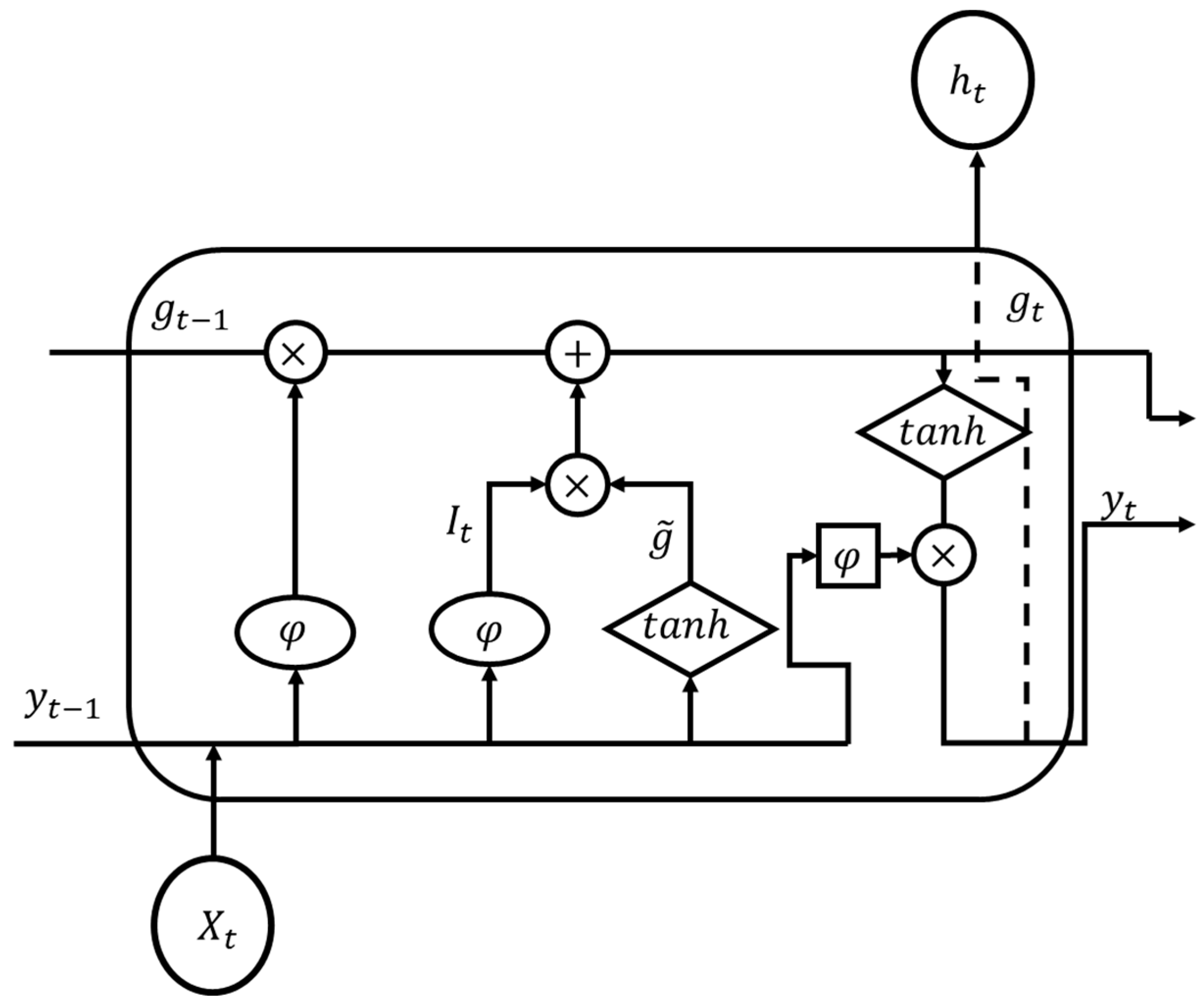
2.1. LSTM
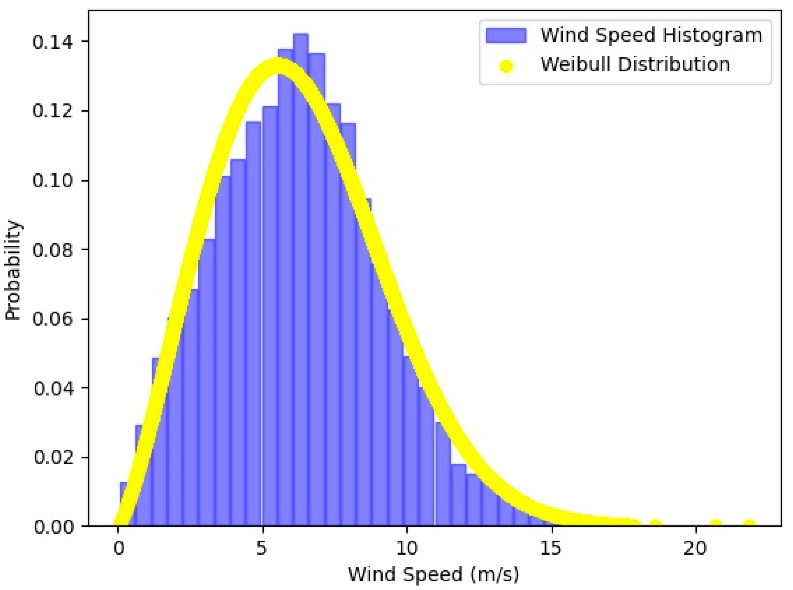
2.2. Weibull Distribution
2.3. SARIMAX
2.4. NWP Model
2.5. Hybrid Model
2.6. Preprocessing and Evaluation Metrics
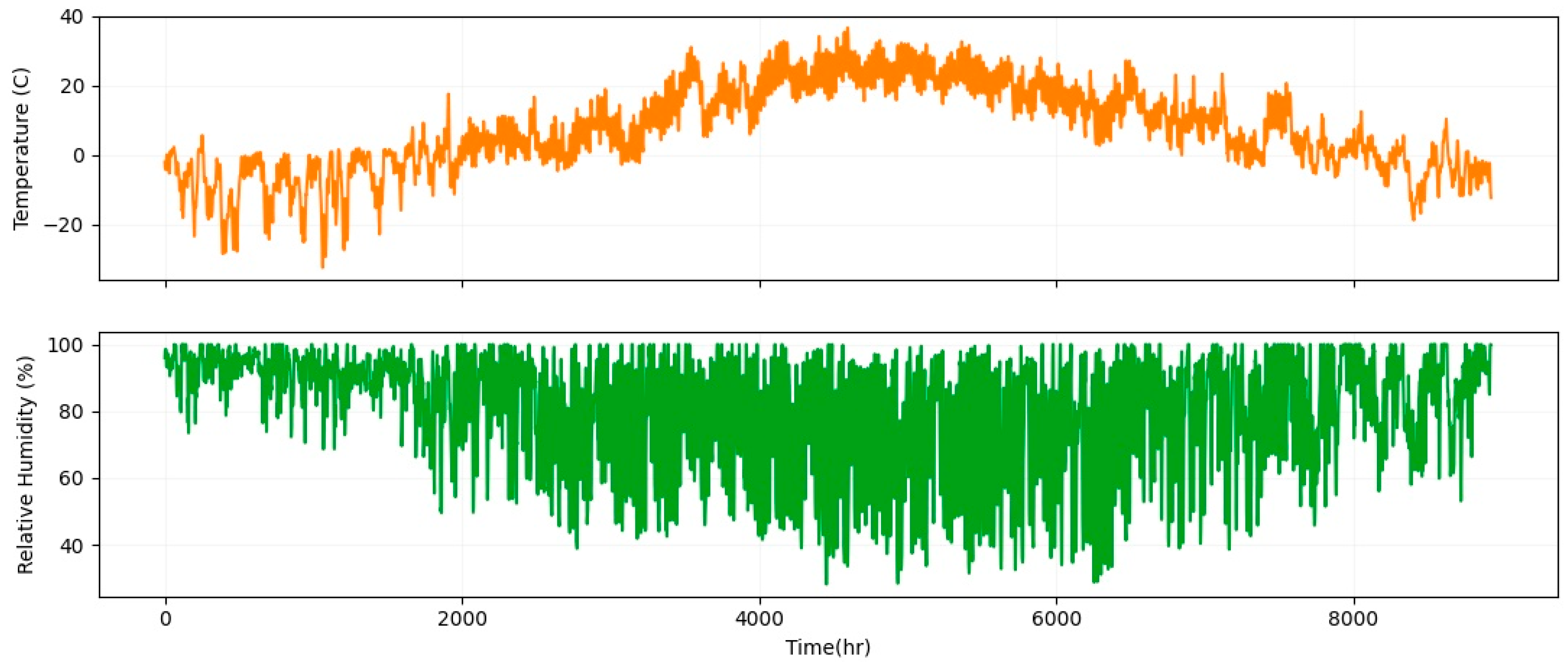
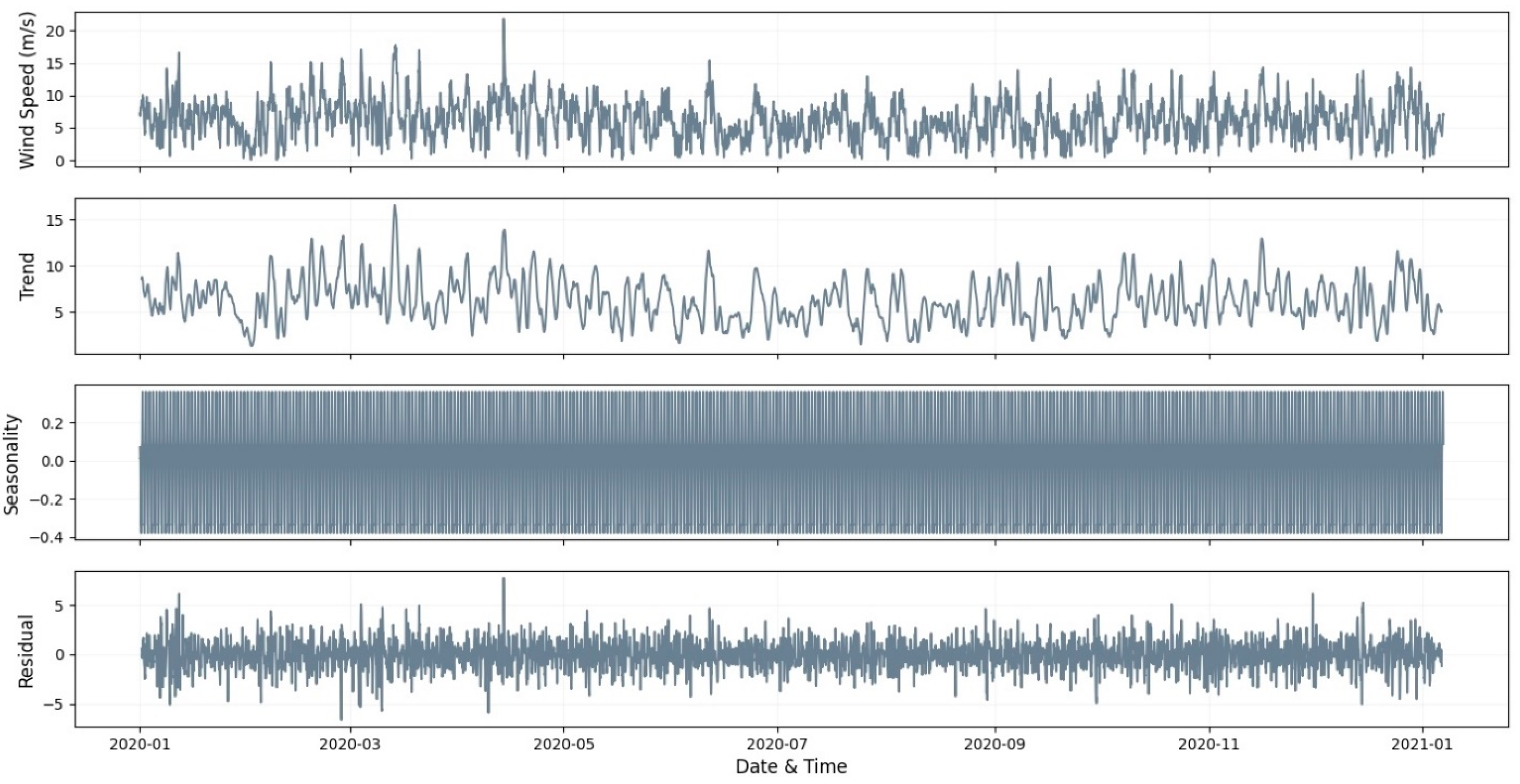
3. Case Study and Data Characteristics
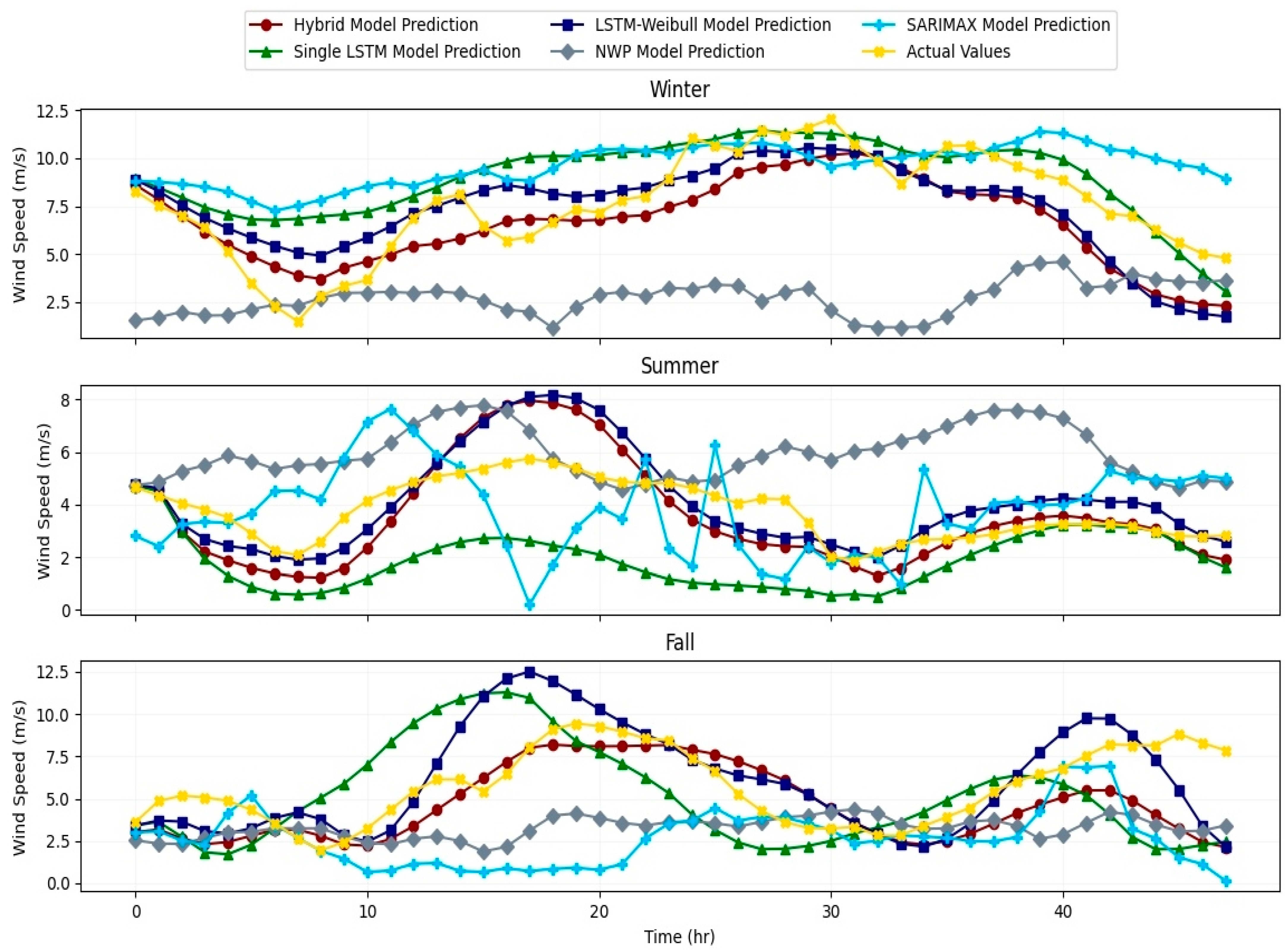
4. Results
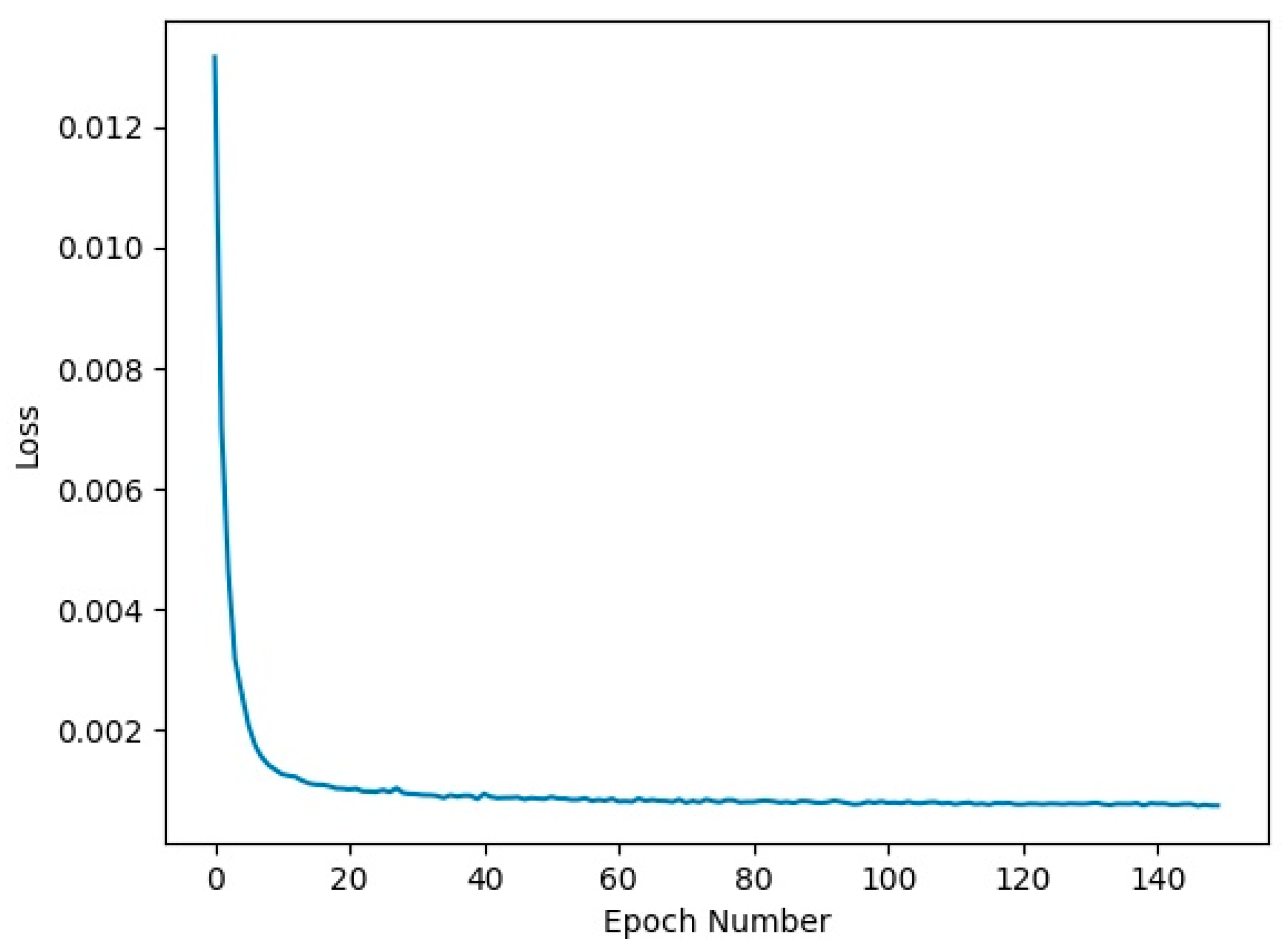
4.1. Implementation
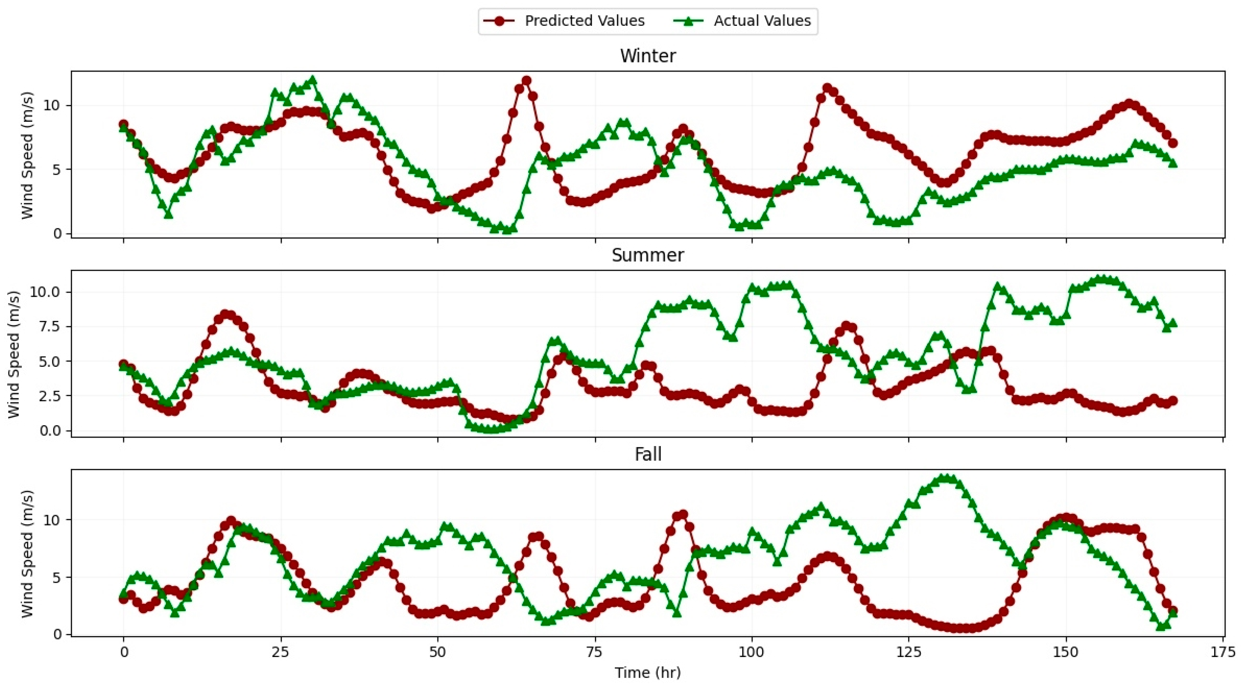
4.2. Discussion
5. Validation
6. Conclusions
Author Contributions
Funding
Data Availability Statement
Acknowledgments
Conflicts of Interest
References
- Worldwide Wind Capacity Reaches 744 Gigawatts–An Unprecedented 93 Gigawatts Added in 2020-World Wind Energy Association. Available online: https://wwindea.org/worldwide-wind-capacity-reaches-744-gigawatts/ (accessed on 1 September 2021).
- Yan, J.; Zhang, H.; Liu, Y.; Han, S.; Li, L.; Lu, Z. Forecasting the High Penetration of Wind Power on Multiple Scales Using Multi-to-Multi Mapping. IEEE Trans. Power Syst. 2018, 33, 3276–3284. [Google Scholar] [CrossRef]
- Cadenas, E.; Rivera, W. Wind speed forecasting in three different regions of Mexico, using a hybrid ARIMA–ANN model. Renew. Energy 2010, 35, 2732–2738. [Google Scholar] [CrossRef]
- Wang, J.; Xiong, S. A hybrid forecasting model based on outlier detection and fuzzy time series—A case study on Hainan wind farm of China. Energy 2014, 76, 526–541. [Google Scholar] [CrossRef]
- Yatiyana, E.; Rajakaruna, S.; Ghosh, A. Wind speed and direction forecasting for wind power generation using ARIMA model. In Proceedings of the 2017 Australasian Universities Power Engineering Conference, AUPEC, Melbourne, VIC, Australia, 19–22 November 2017; pp. 1–6. [Google Scholar] [CrossRef]
- Kavasseri, R.G.; Seetharaman, K. Day-ahead wind speed forecasting using f-ARIMA models. Renew. Energy 2009, 34, 1388–1393. [Google Scholar] [CrossRef]
- Wang, J.; Hu, J.; Ma, K.; Zhang, Y. A self-adaptive hybrid approach for wind speed forecasting. Renew. Energy 2015, 78, 374–385. [Google Scholar] [CrossRef]
- Haque, A.U.; Meng, J. Short-Term Wind Speed Forecasting Based on Fuzzy Artmap. Int. J. Green Energy 2011, 8, 65–80. [Google Scholar] [CrossRef]
- An, S.; Shi, H.; Hu, Q.; Li, X.; Dang, J. Fuzzy rough regression with application to wind speed prediction. Inf. Sci. 2014, 282, 388–400. [Google Scholar] [CrossRef]
- Zhou, J.Y.; Shi, J.; Li, G. Fine tuning support vector machines for short-term wind speed forecasting. Energy Convers. Manag. 2011, 52, 1990–1998. [Google Scholar] [CrossRef]
- Fu, X.; Feng, Z.; Yao, X.; Liu, W. A Novel Twin Support Vector Regression Model for Wind Speed Time-Series Interval Prediction. Energies 2023, 16, 5656. [Google Scholar] [CrossRef]
- Nair, K.R.; Vanitha, V.; Jisma, M. Forecasting of wind speed using ANN, ARIMA and Hybrid models. In Proceedings of the 2017 International Conference on Intelligent Computing, Instrumentation and Control Technologies, ICICICT, Kerala, India, 6–7 July 2017; pp. 170–175. [Google Scholar] [CrossRef]
- Kuremoto, T.; Kimura, S.; Kobayashi, K.; Obayashi, M. Time series forecasting using a deep belief network with restricted Boltzmann machines. Neurocomputing 2014, 137, 47–56. [Google Scholar] [CrossRef]
- Wang, H.; Wang, G.; Li, G.; Peng, J.; Liu, Y. Deep belief network based deterministic and probabilistic wind speed forecasting approach. Appl. Energy 2016, 182, 80–93. [Google Scholar] [CrossRef]
- Wang, H.-Z.; Li, G.-Q.; Wang, G.-B.; Peng, J.-C.; Jiang, H.; Liu, Y.-T. Deep learning based ensemble approach for probabilistic wind power forecasting. Appl. Energy 2017, 188, 56–70. [Google Scholar] [CrossRef]
- Khadem, S.A.; Rey, A.D. Nucleation and growth of cholesteric collagen tactoids: A time-series statistical analysis based on integration of direct numerical simulation (DNS) and long short-term memory recurrent neural network (LSTM-RNN). J. Colloid Interface Sci. 2021, 582, 859–873. [Google Scholar] [CrossRef]
- Liu, H.; Mi, X.-W.; Li, Y.-F. Wind speed forecasting method based on deep learning strategy using empirical wavelet transform, long short term memory neural network and Elman neural network. Energy Convers. Manag. 2018, 156, 498–514. [Google Scholar] [CrossRef]
- Jung, J.; Broadwater, R.P. Current status and future advances for wind speed and power forecasting. Renew. Sustain. Energy Rev. 2014, 31, 762–777. [Google Scholar] [CrossRef]
- Bessac, J.; Constantinescu, E.; Anitescu, M. Stochastic simulation of predictive space–time scenarios of wind speed using observations and physical model outputs. Ann. Appl. Stat. 2018, 12, 432–458. [Google Scholar] [CrossRef]
- Hu, S.; Xiang, Y.; Zhang, H.; Xie, S.; Li, J.; Gu, C.; Sun, W.; Liu, J. Hybrid forecasting method for wind power integrating spatial correlation and corrected numerical weather prediction. Appl. Energy 2021, 293, 116951. [Google Scholar] [CrossRef]
- Jozefowicz, R.; Zaremba, W.; Sutskever, I. An empirical exploration of Recurrent Network architectures. In Proceedings of the 32nd International Conference on Machine Learning, ICML, Lille, France, 6–11 July 2015; Volume 3, pp. 2332–2340. [Google Scholar]
- Koutník, J.; Greff, K.; Gomez, F.; Schmidhuber, J. A clockwork RNN. In Proceedings of the 31st International Conference on Machine Learning, ICML, Beijing, China, 21–26 June 2014; Volume 5, pp. 3881–3889. [Google Scholar]
- Greff, K.; Srivastava, R.K.; Koutník, J.; Steunebrink, B.R.; Schmidhuber, J. LSTM: A Search Space Odyssey. IEEE Trans. Neural Netw. Learn. Syst. 2017, 28, 2222–2232. [Google Scholar] [CrossRef]
- Hochreiter, S. Untersuchungen zu Dynamischen Neuronalen Netzen. Master’s Thesis, Institut Für Informatik, Technische Universität, Munchen, Germany, 1991; pp. 1–71. [Google Scholar]
- Bengio, Y.; Simard, P.; Frasconi, P. Learning long-term dependencies with gradient descent is difficult. IEEE Trans. Neural Networks 1994, 5, 157–166. [Google Scholar] [CrossRef] [PubMed]
- Hochreiter, S.; Schmidhuber, J. Long short-term memory. Neural Comput. 1997, 9, 1735–1780. [Google Scholar] [CrossRef]
- Rahman, A.; Srikumar, V.; Smith, A.D. Predicting electricity consumption for commercial and residential buildings using deep recurrent neural networks. Appl. Energy 2018, 212, 372–385. [Google Scholar] [CrossRef]
- Wen, L.; Zhou, K.; Yang, S.; Lu, X. Optimal load dispatch of community microgrid with deep learning based solar power and load forecasting. Energy 2019, 171, 1053–1065. [Google Scholar] [CrossRef]
- Ozay, C.; Celiktas, M.S. Statistical analysis of wind speed using two-parameter Weibull distribution in Alaçatı region. Energy Convers. Manag. 2016, 121, 49–54. [Google Scholar] [CrossRef]
- Kadhem, A.A.; Wahab, N.I.A.; Aris, I.; Jasni, J.; Abdalla, A.N. Advanced Wind Speed Prediction Model Based on a Combination of Weibull Distribution and an Artificial Neural Network. Energies 2017, 10, 1744. [Google Scholar] [CrossRef]
- Odo, F.C.; Offiah, S.U.; Ugwuoke, P.E. Weibull distribution-based model for prediction of wind potential in Enugu, Nigeria. Adv. Appl. Sci. Res. 2012, 3, 1202–1208. [Google Scholar]
- Alencar, D.B.; Affonso, C.M.; Oliveira, R.C.L.; Filho, J.C.R. Hybrid Approach Combining SARIMA and Neural Networks for Multi-Step Ahead Wind Speed Forecasting in Brazil. IEEE Access 2018, 6, 55986–55994. [Google Scholar] [CrossRef]
- Chen, Y.; Tjandra, S. Daily Collision Prediction with SARIMAX and Generalized Linear Models on the Basis of Temporal and Weather Variables. Transp. Res. Rec. J. Transp. Res. Board 2014, 2432, 26–36. [Google Scholar] [CrossRef]
- Arunraj, N.S.; Ahrens, D.; Fernandes, M. Application of SARIMAX Model to Forecast Daily Sales in Food Retail Industry. Int. J. Oper. Res. Inf. Syst. 2016, 7, 1–21. [Google Scholar] [CrossRef]
- Where Is Montreal, Quebec, Canada on Map Lat Long Coordinates. Available online: https://www.latlong.net/place/montreal-quebec-canada-27653.html (accessed on 30 May 2021).
- NASA POWER|Prediction of Worldwide Energy Resources. Available online: https://power.larc.nasa.gov/ (accessed on 11 April 2022).
- Valdivia-Bautista, S.M.; Domínguez-Navarro, J.A.; Pérez-Cisneros, M.; Vega-Gómez, C.J.; Castillo-Téllez, B. Artificial Intelligence in Wind Speed Forecasting: A Review. Energies 2023, 16, 2457. [Google Scholar] [CrossRef]
- Yang, X.; Xiao, Y.; Chen, S. Wind speed and generated power forecasting in wind farm. Proc. Chin. Soc. Electr. Eng. 2005, 25, 1. [Google Scholar]


| Parameters | Values/Types | Hyper Parameter Optimization Results |
|---|---|---|
| No. hidden layers | 3 | - |
| No. neurons per hidden layer | 60 | - |
| Activation function | Sigmoid | - |
| Optimizer types | {Adam, RMSprop} | Adam |
| Batch size | {1,32,64} | 32 |
| No. of epochs | {50,80,100,110,125,150} | 150 |
| Combination | AIC | Combination | AIC |
|---|---|---|---|
| (0,0,0)(0,1,0,24) | 11,271 | (1,0,1)(2,1,0,24) | 4044 |
| (1,0,0)(1,1,0,24) | 4955 | (2,0,1)(2,1,0,24) | 3959 |
| (1,0,0)(0,1,0,24) | 5548 | (3,0,1)(2,1,0,24) | 3961 |
| (1,0,0)(2,1,0,24) | 4709 | (2,0,2)(2,1,0,24) | 4221 |
| (0,0,0)(2,1,0,24) | 10,553 | (1,0,0)(2,1,0,24) | 4707 |
| (2,0,0)(2,1,0,24) | 3998 | (1,0,2)(2,1,0,24) | 3972 |
| (2,0,0)(1,1,0,24) | 4211 | (3,0,0)(2,1,0,24) | 3962 |
| (3,0,0)(2,1,0,24) | 3964 | (3,0,2)(2,1,0,24) | 3963 |
| (3,0,0)(1,1,0,24) | 4175 | (4,0,1)(2,1,0,24) | 3963 |
| (5,0,0)(2,1,0,24) | 3965 | (3,0,1)(1,1,0,24) | 4176 |
| Parameter/Metric | Value/Type |
|---|---|
| Optimum non-seasonal orders | (2,0,1) |
| Optimum seasonal orders | (2,1,0,24) |
| No. of observations | 2160 |
| Log likelihood | −4270.623 |
| AIC | 3959.516 |
| BIC | 4004.849 |
| HQIC | 3976.106 |
| Covariance type | Outer Product of Gradients (OPG) |
| Model | RMSE | MAE | MSLE |
|---|---|---|---|
| July (Summer) | |||
| LSTM | 2.21 | 1.86 | 0.395 |
| SARIMAX | 2.64 | 2.24 | 0.234 |
| NWP | 2.02 | 1.70 | 0.227 |
| Integrated LSTM–Weibull | 1.35 | 1.12 | 0.071 |
| Hybrid LSTM–Weibull–NWP | 1.18 | 0.95 | 0.066 |
| December (Winter) | |||
| LSTM | 2.14 | 1.63 | 0.106 |
| SARIMAX | 2.81 | 2.3 | 0.155 |
| NWP | 5.58 | 4.90 | 0.849 |
| Integrated LSTM–Weibull | 1.87 | 1.55 | 0.110 |
| Hybrid LSTM–Weibull–NWP | 1.78 | 1.50 | 0.078 |
| October (Fall) | |||
| LSTM | 3.16 | 2.58 | 0.272 |
| SARIMAX | 2.25 | 2.73 | 0.294 |
| NWP | 4.14 | 3.11 | 0.799 |
| Integrated LSTM–Weibull | 2.18 | 1.60 | 0.100 |
| Hybrid LSTM–Weibull–NWP | 2.16 | 1.67 | 0.139 |
Disclaimer/Publisher’s Note: The statements, opinions and data contained in all publications are solely those of the individual author(s) and contributor(s) and not of MDPI and/or the editor(s). MDPI and/or the editor(s) disclaim responsibility for any injury to people or property resulting from any ideas, methods, instructions or products referred to in the content. |
© 2023 by the authors. Licensee MDPI, Basel, Switzerland. This article is an open access article distributed under the terms and conditions of the Creative Commons Attribution (CC BY) license (https://creativecommons.org/licenses/by/4.0/).
Share and Cite
Shirzadi, N.; Nasiri, F.; Menon, R.P.; Monsalvete, P.; Kaifel, A.; Eicker, U. Smart Urban Wind Power Forecasting: Integrating Weibull Distribution, Recurrent Neural Networks, and Numerical Weather Prediction. Energies 2023, 16, 6208. https://doi.org/10.3390/en16176208
Shirzadi N, Nasiri F, Menon RP, Monsalvete P, Kaifel A, Eicker U. Smart Urban Wind Power Forecasting: Integrating Weibull Distribution, Recurrent Neural Networks, and Numerical Weather Prediction. Energies. 2023; 16(17):6208. https://doi.org/10.3390/en16176208
Chicago/Turabian StyleShirzadi, Navid, Fuzhan Nasiri, Ramanunni Parakkal Menon, Pilar Monsalvete, Anton Kaifel, and Ursula Eicker. 2023. "Smart Urban Wind Power Forecasting: Integrating Weibull Distribution, Recurrent Neural Networks, and Numerical Weather Prediction" Energies 16, no. 17: 6208. https://doi.org/10.3390/en16176208
APA StyleShirzadi, N., Nasiri, F., Menon, R. P., Monsalvete, P., Kaifel, A., & Eicker, U. (2023). Smart Urban Wind Power Forecasting: Integrating Weibull Distribution, Recurrent Neural Networks, and Numerical Weather Prediction. Energies, 16(17), 6208. https://doi.org/10.3390/en16176208